Effective operators and vacuum instability as heralds of new physics

For a light enough Higgs boson, the effective potential of the Standard Model develops a dangerous instability at some high energy scale, $\Lambda$, signalling the need for new physics below that scale. On the other hand, a typical low-energy remnant of new physics at some heavy scale, $M$, is the presence of effective non-renormalizable operators (NROs), suppressed by powers of $1/M$. It has been claimed that such operators may modify the behaviour of the effective potential, in such a way as to significantly lower the instability scale. We critically reanalyze the interplay between non-renormalizable operators and vacuum instabilities and find that, contrary to these claims, the effect of NROs on instability bounds is generically small whenever it can be reliably computed.

December 2001

McGill-01/27

SHEP 02-01

IFT-UAM/CSIC-01-41

hep-ph/0201160

It is well known that the Higgs effective potential in the Standard Model (SM) develops an instability if the Higgs mass is below some critical value, termed the vacuum stability bound [1, 2, 3, 4]. This potential instability appears due to the fact that the Higgs quartic coupling, $\lambda$, which is positive at the electroweak scale (where it determines the Higgs mass), can run towards negative values in the ultraviolet (due to radiative corrections from top-quark loops). If this happens at some high energy scale $\Lambda$, for values of the Higgs field $H\sim\Lambda$, the potential is dominated by the negative $\lambda|H|^{4}$ term and it is either unbounded from below or develops a very deep minimum (deeper than the electroweak vacuum) beyond $\Lambda$.

For a given cut-off scale $\Lambda$ one can compute the critical value of the Higgs mass, $M_{h}^{*}(\Lambda)$, below which the potential will develop an instability at, or below, $\Lambda$. As an example, for a top-quark mass $M_{t}=175$ GeV, the stability bound is $M_{h}^{*}\simeq 50$ GeV for $\Lambda=1$ TeV and $M_{h}^{*}\simeq 130$ GeV for $\Lambda=10^{19}$ GeV [2]. Alternatively, for $M_{t}=175$ GeV and $M_{h}=115.6$ GeV (as suggested by LEP2 [7]), the Higgs potential of the Standard Model develops an instability at the scale $\Lambda^{*}\simeq 100$ TeV [2].

The significance of these analyses is that such an instability provides circumstantial evidence for the presence of new physics at energies which cannot be made arbitrarily large compared to the electroweak scale, $v=246$ GeV. This evidence relies on the modern picture of the SM as the low-energy approximation to a more complete theory, with the full theory deviating in its predictions from those of the SM only by powers of $E/M$, where $E$ is the energy of the observable of interest, and where $M$ is the mass scale of the new physics. Viewing the SM prediction of vacuum instability as a failure to reproduce the vacuum properties of this more complete theory for energies $E\sim\Lambda^{*}$, we must conclude that the parameter controlling the difference between these two theories, $\Lambda^{*}/M$, cannot be too small.

Of course $\Lambda^{*}$ as defined by the stability analysis only gives an indication of where the scale, $M$, of new physics must lie, and does not provide a strict upper bound. It is quite possible that the scale $M$ – defined, say, as the mass of the lightest hitherto-undiscovered particle – is a bit larger than $\Lambda^{*}$ [8, 9]. For instance, in the examples explored by Ref. [9] (using a toy model with parameters that mimic those of the MSSM) the mass-scale of the perturbative new physics can be as large as $M=4\Lambda^{*}$.

It is well known that integrating out new physics having mass $M$ generates a host of non-renormalizable operators (NROs) in the effective theory, which are suppressed by powers of $1/M$ and which express in detail how the full theory differs from the SM at low energies, $E\ll M$. It has been remarked by several authors that such operators also contribute to the Higgs potential, $V$, in a way which might affect the vacuum stability bounds. For instance the appearance of a NRO of the form

$$\delta V=-{\alpha\over 3M^{2}}|H|^{6}\ ,$$ (1)

changes the behaviour of $V$ by an amount which is small for small $H$, but which might nonetheless successfully compete with equally small perturbative SM effects. By including such a term in the Higgs potential, refs. [11, 12] in this way find the vacuum instability to arise for scales $\Lambda^{*}_{\alpha}$ which can be a few orders of magnitude smaller than in the absence of terms like eq. (1).

It is our purpose in this letter to critically re-examine these arguments. We argue that large changes to $\Lambda^{*}$ typically indicate a breakdown of the approximations being used, rather than providing a solid indication that new physics must exist at comparatively low energies. For simplicity we limit our analysis to a single non-renormalizable operator of the form (1), and take $\alpha\geq 0$ (which is the case of interest because, as we will see, it tends to lower the instability scale). Although one generally expects a host of different NROs to arise when integrating out heavy physics, our main conclusions are not substantially affected by the presence of these other effective operators.

We present our arguments in the following way. In section 1 we reproduce previous studies which find sizable changes to $\Lambda^{*}$ due to this interplay between stability bounds and non-renormalizable operators. In section 2, we explain, with the help of a toy model, the dangers of using an effective theory (valid below some cut-off) to study properties of the effective potential at values of the field close to the cut-off.

In section 3 we present our alternative, ’bottom-up’, approach to this problem: assuming that we know $M_{h}$ and have indications of the existence of a NRO like (1), we first examine how the value of $M$ in (1) can be estimated. We then show how the calculation of the instability scale $\Lambda^{*}$ changes due to the NRO of eq. (1). We consider in turn the three mutually-exclusive and exhaustive cases for the relative sizes of the new physics scales, $M$ and $\Lambda^{*}$: (a) $\Lambda^{*}\gg M$, (b) $\Lambda^{*}\simeq M$ and (c) $\Lambda^{*}\ll M$. [Here $\Lambda^{*}$ is the instability scale in the pure SM, without NROs, and $M$ is the new physics scale appearing in (1)]. We show that only case (c) can be studied reliably in an effective theory approach, and we conclude that the change in $\Lambda^{*}$ due to the NRO (1) is in general small when its effects are reliably calculable. We discuss separately the particular choices of parameters – $M_{h}\sim 120-130$ GeV (the precise value depends on $M_{t}$ and the strong coupling constant $\alpha_{s}$) – that require some qualifications, but which do not change our conclusion.

1. Previous Analyses: References [11, 12] study in detail the possible influence of non-renormalizable operators (in the Higgs potential) on vacuum stability bounds. Although they proceed with different levels of sophistication (e.g. ref. [12] includes the influence of NROs on the renormalization group evolution of the parameters, an effect that was not considered in ref. [11]) both find that non-renormalizable terms, like the one presented in eq. (1), do have a significant impact on stability bounds.

There are two (equivalent) ways of stating their results:

• A) For a given value of the cut-off scale $\Lambda$, the corresponding value of the stability bound on the Higgs mass, $M_{h}^{*}(\Lambda)$, can be relaxed (i.e. the bound increases) quite significantly due to the presence of non-renormalizable operators like (1);

• B) For a fixed value of the Higgs mass, the scale $\Lambda^{*}$ at which the Higgs potential develops an instability can be lowered dramatically by the presence of non-renormalizable operators like (1).

These results are obtained as follows. Let us assume for simplicity that the only NRO present is of the form given by equation (1), with $\alpha>0$ (as already mentioned, we focus on this sign for $\alpha$ because we are more interested in effects that lower the scale of new physics). For a fixed $\Lambda$, the stability bound in the pure SM, $M_{h}^{*}(\Lambda)\equiv M_{h}^{*}(\Lambda,\alpha=0)$, is obtained [1, 2, 3, 4] by setting $\lambda(Q=\Lambda)\simeq 0$ (where $Q$ is the renormalization scale) as a boundary condition. More precisely we require

$$\left.\hat{\lambda}(Q)\equiv\left[\lambda(Q)+\delta\lambda\right]\right|_{Q=\Lambda}=0\ ,$$ (2)

where $\delta\lambda$ is a (non-logarithmic) correction of one-loop order. In our definion, $\hat{\lambda}(Q)$ is simply the quartic Higgs coupling in the one-loop potential evaluated at $Q=|H|$ and it tracks the zeroes of $V$ for large $|H|$. This quantity differs slightly from a similar one-loop corrected $\tilde{\lambda}(Q)$ used in Ref. [2] that tracks instead the extrema of $V$. Condition (2) ensures $V(Q=\Lambda)\simeq\hat{\lambda}(\Lambda)|H|^{4}/2\simeq 0$ near $|H|\sim\Lambda$.

For $\alpha\neq 0$ and positive, however, one has to deal also with the $|H|^{6}$-term, which may be competitive with the $|H|^{4}$-term in spite of the $M^{-2}$ suppression of the former. If $M\simeq\Lambda$ (more about this later) we are led to the approximate condition (for borderline stability)

$${1\over 2}\hat{\lambda}_{\alpha}(Q)\equiv\left[{1\over 2}\hat{\lambda}(Q)-{1\over 3}\alpha(Q)\left.{|H|^{2}\over\Lambda^{2}}\right]\right|_{Q=\Lambda}\simeq 0\ ,$$ (3)

for $|H|\simeq\Lambda$. That is, the boundary condition for $\lambda$ will be

$$\lambda(\Lambda)\simeq-\delta\lambda+{2\over 3}\alpha(\Lambda)=0\ .$$ (4)

Comparing (4) to (2), and noting that a larger value of $\lambda$ at the scale $\Lambda$ translates into a larger value at the electroweak scale, we arrive at $M_{h}^{*}(\Lambda,\alpha)\geq M_{h}^{*}(\Lambda,\alpha=0)$. This conforms to statement (A) above. For $\Lambda\stackrel{{\scriptstyle<}}{{{}_{\sim}}}50$ TeV, the increase in $M_{h}^{*}(\Lambda,\alpha)$ for moderate values of $\alpha$ is claimed [12] to be $\sim 40-60$ GeV, which is a rather large effect.

Alternatively, for a fixed value of $M_{h}$, the instability scale in the SM, $\Lambda^{*}(M_{h})$, is determined by condition (2). For a non-zero $\alpha>0$, however, the potential seems to run into an instability as soon as $\lambda(Q)$ is so small that $\lambda|H|^{4}$ cannot compete any more with the negative term $-\alpha|H|^{6}$. So, the new instability scale must satisfy $\Lambda^{*}_{\alpha}\equiv\Lambda^{*}(M_{h},\alpha)<\Lambda^{*}(M_{h},\alpha=0)$ as stated in (B) above. For $M_{h}\simeq 115.6$ GeV (as suggested by LEP [7]) the instability scale in the pure SM, $\Lambda^{*}\simeq 100$ TeV, would be lowered by this argument, according to [12], to $\Lambda^{*}_{\alpha}\simeq 1-20$ TeV depending on $\alpha$. This is again a rather dramatic downward shift.

2. The Expansion of $V$ in Powers of $H$$/$$M$: The large size of the corrections obtained by the previous arguments is troubling from the point of view of the effective theory, since the validity of the low-energy expansion itself usually ensures that the effects of NROs are small corrections to the predictions of the renormalizable low-energy theory. If NROs substantially can change the predictions of the SM in this instance, we must ask why the same is not true in other situations for which the SM seems to work well. In other instances where similarly large results from effective NROs were found, the conclusions turned out to be artifacts of applying the effective theory outside its domain of validity [13].

For an indication of what is going on, recall the assumption made in the derivation that $H\simeq\Lambda\simeq M$, since one might under these circumstances question the expansion of the scalar potential in powers of $H/M$. Indeed, the dangers of making this kind of expansion in a stability analysis may be illustrated by the following toy model. Consider two real scalar fields, $\phi$ and $\Phi$, with potential

$$V(\phi,\Phi)=-{1\over 2}m^{2}\phi^{2}+{1\over 8}\lambda\phi^{4}+{1\over 2}M^{2}\Phi^{2}+\xi\phi^{3}\Phi+\kappa\phi^{2}\Phi^{2}\ ,$$ (5)

and take $M^{2}\gg m^{2}>0$. The light field, $\phi$, acquires a vacuum expectation value (VEV), $\langle\phi\rangle\sim-m^{2}/\lambda$ and this also triggers a non-zero, but small, VEV for $\Phi$, but these are complications inessential for our purpose.

To ensure that the the potential (5) is not unbounded from below we must choose our parameters in such a way as to ensure

$$\frac{1}{8}\lambda+\xi y+\kappa y^{2}\geq 0$$ (6)

where $y\equiv\Phi/\phi\in(-\infty,\infty)$. This condition is automatically satisfied provided

$$\kappa>0\ ,\;\;\;\;{\mathrm{a}nd}\;\;\;\;\lambda\geq 2\frac{\xi^{2}}{\kappa}\ ,$$ (7)

which is a condition we assume to hold in what follows.

For energies small compared to $M$ we can integrate out the heavy field $\Phi$ to obtain the low-energy potential, which at tree level becomes

$$V(\phi)=-{1\over 2}m^{2}\phi^{2}+{1\over 8}\lambda\phi^{4}-{1\over 2}\xi^{2}{\phi^{6}\over M^{2}+2\kappa\phi^{2}}\ .$$ (8)

If this is expanded in powers of $\phi^{2}/M^{2}$, then the dominant term is precisely of the form (1), with $\alpha=3\,\xi^{2}/2>0$. If we were to truncate the potential (8) at $O(\phi^{6}/M^{2})$ and ignore higher powers of $\phi$, we would conclude that the potential develops an instability when

$${\phi^{2}\over M^{2}}\simeq{\lambda\over 4\xi^{2}}\ ,$$ (9)

due to the negative $\phi^{6}$-contribution. Using (7), it would be tempting to justify the truncation of the potential on a posteori grounds, since (9) implies $(\phi/M)^{2}\geq 1/(2\kappa)$, which can be smaller than 1 for $\kappa\geq 0.5$.

The instability found in this way is specious, however, because we know that it is an artifact of the truncation of the potential to order $\phi^{6}/M^{2}$. This is a bad approximation to the potential, (8), which does not share this instability by virtue of the second of conditions (7), which guarantees the stability of the underlying potential, (5). For values of $\phi$ close to the scale $M$, it is not correct to expand the potential within the effective theory, even if the effective theory itself is perfectly well justified (such as by having $m\ll M$).

How can it be that the effective theory can be justified as an expansion in powers of $1/M$ and yet the potential cannot also be so expanded? This is not so odd as it might seem. The validity of the effective theory rests on the absence of large energy densities, since these might allow the production of the heavy particles which have been integrated out. In our example this justifies the suppression of terms involving powers of $m/M$, and of terms involving higher derivatives divided by powers of $M$. The validity of the expansion of $V(\phi)$ in powers of $\phi/M$ hinges on whether or not fields for which $\phi/M\simeq 1$ can produce an energy density which is small enough to remain within the low-energy regime.

That is, if the scalar potential is sufficiently shallow as a function of $\phi$, it can be that $\phi\simeq M$ and yet $V(\phi)$ remains small. If so, it is illegitimate to expand $V(\phi)$ in powers of $\phi/M$ even within the low-energy theory. This situation frequently arises within supergravity theories, for which the scalar potentials often have flat directions. In such cases one keeps in the effective theory the terms with the fewest derivatives (such as the Einstein-Hilbert action) but also finds nonpolynomial scalar potentials.

The Higgs potential of the SM does not have such a flat direction, since the quartic interaction generically ensures that fields $H\simeq M$ produce energy densities of order $V(H)\simeq\lambda M^{4}$. This is why it is generally a good approximation to expand the SM potential in powers of $H/M$, keeping only the renormalizable terms. The exception to these statement arises precisely in the instance of marginal stability, when the quartic coupling is close to vanishing: the case of interest of the previous analysis. In this case field configurations $H\simeq M$, by assumption, do not cost prohibitive energy to excite.

In all cases, the effective theory faithfully reproduces the vacuum behaviour of the underlying theory to which it is an approximation. If the ground state energy in this underlying theory has flat directions (or any generic field region) which cost little energy, then the potential in the effective theory will be nonpolynomial, but stable. If, on the other hand, the underlying energy has no shallow directions, the effective potential will be well approximated by its expansion in powers of $H$ about the vacuum.

3. A Revised Analysis: Based on the insights suggested by the toy model, we may now reanalyze the stability analysis within the SM supplemented by NROs in the Higgs potential. For the purposes of the analysis we adopt the point of view that, sometime into the future, the Higgs particle has been discovered and the value of the Higgs mass is known. We also assume that although no new physics beyond the SM has been observed directly, Higgs scattering is sufficiently well measured that there is indirect evidence for new physics through a non-renormalizable $|H|^{6}$ interaction in the Higgs potential.

In this scenario the scale $M$, need not a priori be related to the scale $\Lambda^{*}$ suggested by the SM stability analysis. We therefore consider three different cases according to whether $M$ is smaller than, comparable to, or larger than the instability scale $\Lambda^{*}(M_{h})$ in the pure SM. This is in contrast with the analyses in refs. [11, 12], which always assume $M\simeq\Lambda$.

In all discussions about the relative sizes of the scales $M$ and $\Lambda^{*}$ one must bear in mind that the low-energy theory does not allow a separate determination of $M$ and the coupling $\alpha$ which appear in the combination $\alpha\,|H|^{6}/M^{2}$. For instance, if such a sextic term were generated at tree level by the exchange of a heavy scalar, $S$, having a coupling $gSH^{3}$, then $\alpha\sim g^{2}$. If, however, it is generated at one loop by the circulation of a heavy fermion of mass $M$ we would expect $\alpha\sim y^{6}/(4\pi)^{2}$, where $y$ is the heavy-particle/Higgs Yukawa coupling. Strongly coupled physics might generate $\alpha\sim{\cal O}(1)$. Clearly in the cases where $\alpha\ll 1$, the scale indicated by the coefficient of the $|H|^{6}$ term, $M/\sqrt{\alpha}$, can be much larger than the the actual mass, $M$, of the virtual particle which is responsible for this term.

3.1. The case ${\mbox{\boldmath{$M$}}}{\mbox{\boldmath{$\ll$}}}{\mbox{\boldmath{$\Lambda$}}}^{\mbox{\boldmath{$*$}}}{\mbox{\boldmath{$($}}}{\mbox{\boldmath{$M$}}}_{\mbox{\boldmath{$h$}}}\mbox{\boldmath{$)$}}$. This is interesting by itself, to the extent that the new physics that generates $|H|^{6}$ is much closer to the electroweak scale than anticipated by the instability analysis. Of course, the fact that new physics appears below $\Lambda^{*}$ is consistent with the expectations derived from the pathological behaviour of the potential at $\Lambda^{*}$ (i.e. some new physics at, or below, $\Lambda^{*}$ should cure that pathology).

In any case, once there is evidence for new physics at scales $M\ll\Lambda^{*}$ coupled to the Higgs sector, there need not be any new physics at the scale $\Lambda^{*}$ at all. After all, our only evidence that something happens at $\Lambda^{*}$ relies on using the low-energy Higgs potential in a stability analysis at this scale, and we have no justification for believing this potential is a good approximation above the scale $M$. A reliable determination of the instability scale must wait until the theory that describes the physics at scales of order $M$ is worked out. We see that the case $M\ll\Lambda^{*}$ eliminates the instability question from the list of real problems of the model, in the same sense that the appearance of a Landau pole in the electromagnetic coupling at a scale much larger than the Planck scale is not a real problem in the SM.

Once the new physics at $M$ is specified, then one can examine whether it modifies the stability bounds or not. This was done, for example, in Ref. [14] for the case in which the new physics is a heavy fourth family and in Ref. [15] for the case of heavy right-handed neutrinos that implement a see-saw mechanism.

3.2. The case ${\mbox{\boldmath{$M$}}}{\mbox{\boldmath{$\simeq$}}}{\mbox{\boldmath{$\Lambda$}}}^{\mbox{\boldmath{$*$}}}{\mbox{\boldmath{$($}}}{\mbox{\boldmath{$M$}}}_{\mbox{\boldmath{$h$}}}\mbox{\boldmath{$)$}}$. This case would be interesting because one would have two independent indications for new physics at the same scale. To the extent that the additional Higgs NROs enter with coefficients which exacerbate the low-energy stabilities – such as a term $-\alpha\,H^{6}$ with $\alpha>0$ – then we know that the vacuum energetics drives $H$ out to values of order $M$, for which the expansion in powers of $H/M$ breaks down.

It is difficult to go much further than this, however, because the breakdown of the $1/M$ expansions removes our only tool for analysis. One needs to know the physics at $M$ to ascertain whether there is an instability in the potential, and at what scale it occurs. This is the low-energy theory’s way of telling us that we are asking a question – the value of $H$ which minimizes the energy – whose answer cannot be reliably obtained purely within an effective theory without reference to the degrees of freedom at scale $M$.

3.3. ${\mbox{\boldmath{$M$}}}{\mbox{\boldmath{$\gg$}}}{\mbox{\boldmath{$\Lambda$}}}^{\mbox{\boldmath{$*$}}}{\mbox{\boldmath{$($}}}{\mbox{\boldmath{$M$}}}_{\mbox{\boldmath{$h$}}}\mbox{\boldmath{$)$}}$. This is the one case for which purely low-energy calculations can reliably determine the influence, if any, of the $|H|^{6}$ term on the calculation of $\Lambda^{*}$. We must recognize that the limit $M\gg\Lambda^{*}$ is somewhat strange, because we know physics at scales $\Lambda^{*}$ must ultimately allow us to understand the stability of the electroweak-breaking minimum of the Higgs potential, but we are assuming this is not done by growing effective $|H|^{6}$ terms with coefficients of order $(1/\Lambda^{*})^{2}$. If we have separate indications for new Higgs-related physics at a larger scale $M$, the odds are that such new physics is unrelated to the physics that cures the instability problem.

Although $M\gg\Lambda^{*}$ is odd, we do not believe it is absolutely impossible. For instance, one might imagine there to be a selection rule in the low-energy theory which forbids the generation of the $|H|^{6}$ term at the scale $\Lambda^{*}$, but not at higher scales $M$ (in much the same way that flavour-changing interactions amongst fermions arise in the low-energy limit in the Standard Model). This might not preclude the appearance at scale $\Lambda^{*}$ of higher powers of $|H|$ than $|H|^{6}$, which would be the precursors in the low-energy potential of the stabilization which happens at this scale. It is difficult to see how a selection rule could do this for an $|H|^{6}$ term (for a single Higgs field) taken in isolation, but it might conceivably arise within a supersymmetric theory, where the scalar potential is generated by a superpotential which can be subject to selection rules and nonrenormalization theorems at scale $\Lambda^{*}$.

In any case, putting aside the issue as to how the low-energy theory arises, we adopt the spirit used in the literature, and simply examine how the prediction for $\Lambda^{*}$ is changed in the low-energy theory by the appearance of an effective $|H|^{6}$ term.

To see how $\Lambda^{*}(M_{h})$ gets modified by $\alpha\neq 0$ we have to determine the balance between the $|H|^{4}$ and $|H|^{6}$ terms in the potential. For $|H|\sim\Lambda^{*}$, the quartic term is

$$\delta_{4}V={1\over 2}[\lambda(Q)+\delta\lambda]|H(Q)|^{4}\ ,$$ (10)

where $Q$ must be chosen as $Q\sim|H|$ and the $Q$-dependence of $\lambda$ and $H$ is governed at one-loop by

$${d\lambda\over d\log Q}\equiv\beta_{\lambda}={1\over 16\pi^{2}}\left[12(\lambda^{2}-h_{t}^{2}+\lambda h_{t}^{2})-(9g^{2}+3{g^{\prime}}^{2})\lambda+{3\over 4}(3g^{4}+2g^{2}{g^{\prime}}^{2}+{g^{\prime}}^{4})\right]\ ,$$ (11)

and

$${d\log|H|\over d\log Q}\equiv\gamma_{H}={1\over 16\pi^{2}}\left[{3\over 4}(3g^{2}+{g^{\prime}}^{2}-4h_{t}^{2})\right]\ ,$$ (12)

where $h_{t}$ is the top-quark Yukawa coupling, and $g,g^{\prime}$ are the $SU(2)_{L}$ and $U(1)_{Y}$ gauge couplings, respectively. We find that, for field values in the neighbourhood of $\Lambda^{*}$ [defined by $\lambda(\Lambda^{*})+\delta\lambda=0$], the quartic term of the potential is given by

$$\delta_{4}V={1\over 2}\beta_{\lambda}(\Lambda^{*})|H|^{4}\left[1+4\gamma_{H}(\Lambda^{*})\log{|H|\over\Lambda^{*}}\right]\log{|H|\over\Lambda^{*}}\ ,$$ (13)

while the non-renormalizable part will have the form

$$\delta_{6}V=-{1\over 3M^{2}}|H|^{6}\left[\alpha(\Lambda^{*})+\beta_{\alpha}(\Lambda^{*})\log{|H|\over\Lambda^{*}}\right]\left[1+6\gamma_{H}(\Lambda^{*})\log{|H|\over\Lambda^{*}}\right]\ ,$$ (14)

where $\beta_{\alpha}\equiv d\alpha/d\log Q$ is given in ref. [12].

The new instability scale $\Lambda^{*}_{\alpha}\equiv\Lambda^{*}(M_{h},\alpha)$ is determined by the condition $\delta_{4}V+\delta_{6}V\simeq 0$, which leads to

$$\beta_{\lambda}(\Lambda^{*})\log{\Lambda^{*}_{\alpha}\over\Lambda^{*}}\simeq{2\over 3}\left({\Lambda^{*}_{\alpha}\over M}\right)^{2}\left[\alpha(\Lambda^{*})+(\beta_{\alpha}+2\alpha\gamma_{H})\log{\Lambda^{*}_{\alpha}\over\Lambda^{*}}\right]\ ,$$ (15)

and this implies

$$\Lambda^{*}_{\alpha}\simeq\Lambda^{*}\exp\left[{2\over 3}{\alpha(\Lambda^{*})\over\beta_{\lambda}}\left({\Lambda^{*}\over M}\right)^{2}\right]\ .$$ (16)

Remembering that $\beta_{\lambda}\leq 0$ (this caused the instability in the first place), eq. (16) shows that the instability scale is decreased slightly by a non-zero positive $\alpha$ (of course, if $\alpha<0$, the instability scale would increase a little).

The Higgs stability bound has a logarithmic sensitivity to $\Lambda$ and therefore the reduction (16) affects very mildly the value of this bound. Its change can be estimated to be

$$\delta{M_{h}^{*}}^{2}\simeq{\alpha(\Lambda^{*})\over 3}\left({\Lambda^{*}\over M}\right)^{2}v^{2}\ ,$$ (17)

where $v\simeq 246$ GeV is the Higgs VEV. For reasonable values of $\alpha(\Lambda^{*})$ this is a very small shift (much smaller than the $\sim 5$ GeV uncertainty due to the indetermination of $\alpha_{s}$ or $h_{t}$).

The only possible caveat in the previous discussion is the possibility of having $\beta_{\lambda}(\Lambda^{*})\simeq 0$. This clearly requires very particular values of the parameters, but in fact it can be arranged, as we explain in what follows. As we have seen, for low enough values of $M_{h}$, $\beta_{\lambda}(M_{W})$ is negative, due to the $-h_{t}^{2}$ term in (11), and drives $\lambda$ towards negative values at higher scales. However, $h_{t}$ decreases with increasing energy, and eventually $\beta_{\lambda}$ turns positive again. This does not solve the instability problem, though, because if $\lambda$ takes negative values in some energy range the potential develops a very deep minimum there and cannot be accepted, even if $\lambda$ is positive at even higher energies [2].

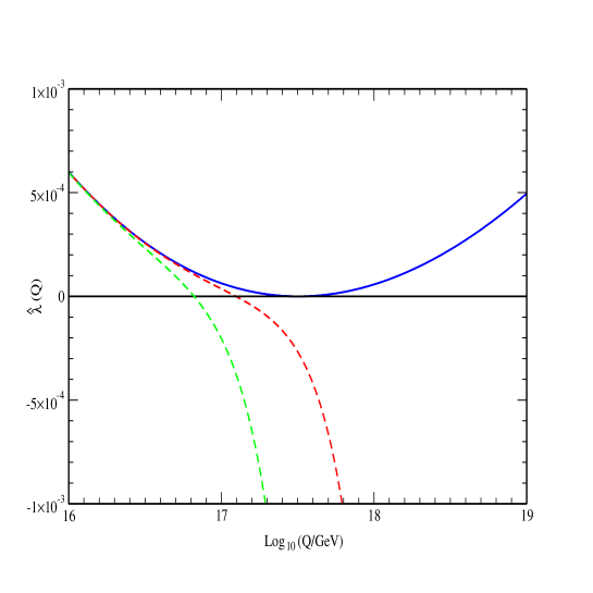
Figure 1: Running $\hat{\lambda}_{\alpha}(Q)$ for the pure SM ($\alpha=0$, solid line) and for the SM with a NRO like (1) with $M=M_{p}$ and $\alpha=0.1$, 1 (dashed lines). Other parameters are: $M_{t}=169.2$ GeV, $\alpha_{s}(M_{Z})=0.12$ and $M_{h}=121.5$ GeV.

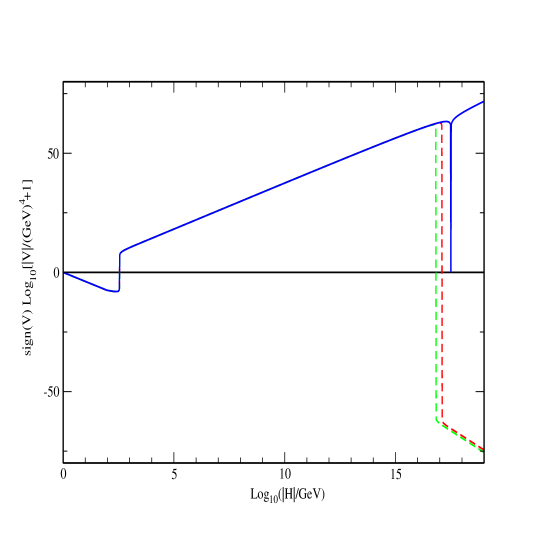
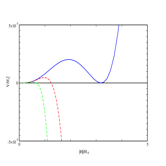
Figure 2: Upper plot: Effective potential corresponding to the parameters of fig. 1, with the same line coding. Lower plot: detail of the instability region.

In any case, what matters now is that, in cases like the ones described in the previous paragraph, there is an energy scale at which $\beta_{\lambda}(Q_{0})\simeq 0$. The case we are after is that in which $\beta_{\lambda}(Q_{0})\simeq 0$ and $\lambda(Q_{0})\simeq 0$, i.e.

$$\beta_{\lambda}(\Lambda^{*})\simeq 0\ .$$ (18)

In table 1, we list the values of $M_{h}$ and $\Lambda^{*}$ for which (18) holds, taking $M_{t}=174.3\pm 5.1$ GeV and $\alpha_{s}(M_{Z})=0.118\pm 0.002$, the current experimental ranges as given in ref. [16]. For all our numerical work, we use the renormalization-group-improved one-loop Higgs potential, with parameters running with two-loop beta-functions (see Ref. [2]). From table 1 we see that condition (18) can only be arranged for rather large values of $\Lambda^{*}$, not far from the Planck Mass. Entries with $\Lambda=M_{p}$ in table 1 correspond to cases that do not satisfy condition (18) for any scale below $M_{p}$. (In other words, for such parameters one would get $\Lambda^{*}>M_{p}$.) The value of $M_{h}$ quoted for these cases is simply the stability bound for $\Lambda=M_{p}$. Figure 1 shows the running of $\hat{\lambda}(Q)$ (solid line) for the extreme case $M_{t}=169.2$ GeV and $\alpha_{s}=0.12$. It is clear that, for values of $M_{h}$ higher than $M_{h}^{*}\simeq 121.5$ GeV (see table 1), the SM potential is free of instabilities at any scale (for these values of $M_{t}$ and $\alpha_{s}$). In this sense, the stability bound associated with cut-off scales $\Lambda$ beyond $\Lambda^{*}\sim 8\times 10^{16}$ GeV is independent of the value of $\Lambda$. This implies, in other words, that [for the previous values of $M_{t}$ and $\alpha_{s}(M_{Z})$] the potential of the SM with cut-off $\Lambda=10^{19}$ GeV, and $M_{h}$ slightly below $M_{h}^{*}\simeq 121.5$ GeV develops an instability around $\Lambda^{*}\sim 8\times 10^{16}$ GeV, well below the cut-off $\Lambda=10^{19}$ GeV.

$\alpha_{s}(M_{Z})\downarrow$  ; $M_{t}$[GeV]$\rightarrow$	169.2	174.3	179.4
0.120	121.5; $3\times 10^{17}$	132; $M_{p}$	142.5; $M_{p}$
0.118	123; $9\times 10^{17}$	133.5; $M_{p}$	144; $M_{p}$
0.116	125; $3\times 10^{18}$	135; $M_{p}$	145; $M_{p}$

Table 1: Values of $\{M_{h};\Lambda^{*}\}$ in GeV, for the indicated values of $\alpha_{s}(M_{Z})$ and $M_{t}$.

Assuming then that we live in such a world, with $M_{t}=169.2$ GeV, $\alpha_{s}(M_{Z})=0.12$ and $M_{h}\simeq 121.5$ GeV, the derivation of $\Lambda^{*}_{\alpha}$ has to be more precise than the one presented before. In particular, we have to keep higher order corrections in the evaluation of $\hat{\lambda}(Q)$ which, around $\Lambda^{*}$, is given by

$$\lambda(Q)\simeq\beta_{\lambda}(\Lambda^{*})\log{Q\over\Lambda^{*}}+{1\over 2}\beta^{\prime}_{\lambda}(\Lambda^{*})\left[\log{Q\over\Lambda^{*}}\right]^{2}+...$$ (19)

where $\beta^{\prime}_{\lambda}\equiv d\beta_{\lambda}/d\log Q$. The first term in the right hand side is now zero, due to our choice of parameters [that ensure $\beta_{\lambda}(\Lambda^{*})=0$]. Using (19), we can compute the new instability scale for non-zero $\alpha$ and find

$$\Lambda_{\alpha}^{*}\simeq\Lambda^{*}\exp\left[-{\Lambda^{*}\over M}\sqrt{{2\alpha(\Lambda^{*})\over 3\beta^{\prime}_{\lambda}(\Lambda^{*})}}\right]\ ,$$ (20)

while (17) is still valid. This shows that the decrease in the instability scale can be larger now, even if the change in the stability bound is still very small.

Figure 1 shows also in dashed lines the running of $\hat{\lambda}_{\alpha}(Q)\equiv\hat{\lambda}(Q)-2\alpha|H|^{2}/(3M^{2})$, quantity that governs the stability of the potential for non-zero $\alpha$. We show two cases with $\alpha=0.1$ and $1.0$ (the curve for $\alpha=0.1$ is closer to the solid, $\alpha=0$, line). Figures 2a and 2b show the potential corresponding to the same choices of parameters made in fig. 1. Fig. 2a presents the potential in a form suitable to show its structure at all scales (i.e. the electroweak vacuum and the non-standard minimum, or instabilities, at $\Lambda^{*}\sim 10^{17}$ GeV). The line coding is as in fig. 1. Figure 2b focuses on the structure of the potential near the instability scale and presents simply $V/H_{0}^{4}$ versus $|H|/H_{0}$ with $H_{0}\equiv 10^{17}$ GeV. Both plots show clearly the instabilities that appear for non-zero $\alpha$, but it is manifest that, even in this particularly sensitive case, the shift $\Lambda^{*}\rightarrow\Lambda_{\alpha}^{*}$ is not larger than an order of magnitude. Alternatively, the stability bound associated to the cut-off scale $\Lambda\simeq 3\times 10^{17}$ GeV for the case $\alpha\neq 0$ (notice that, as explained in previous sections, we cannot compute reliably the stability bound for $\Lambda=M_{p}$ in this case) is nearly indistinguishable from the $\alpha=0$ bound. We have checked that the difference is smaller than 1 GeV.

In summary, we have re-examined the issue of how effective non-renormalizable interactions in the Higgs potential, induced by new physics, can change the understanding of vacuum stability within the low-energy effective theory. We find that calculations which remain within the effective theory’s domain of validity predict only small changes to the instability scale which is inferred purely within the SM.

Because this conclusion disagrees with some previous analyses of these same issues, we have re-examined these analyses and find that they depend on the evaluation of $V$ for fields large enough to invalidate its expansion in powers of $H$. This happens because the large effect is claimed for non-renormalizable interactions whose sign exacerbates any low-energy stability problems. As a result these interactions tend to drive the potential minimum out to fields which are too large to use truncated potentials.

References

-
[1]
N. V. Krasnikov,
Yad. Fiz. 28 (1978) 549 [Sov. J. Nucl. Phys. 28(2)
(1978) 279];
H. D. Politzer and S. Wolfram, Phys. Lett. B 82 (1979) 242 [Erratum-ibid. 83B (1979) 421];
P. Q. Hung, Phys. Rev. Lett. 42 (1979) 873;
N. Cabibbo, L. Maiani, G. Parisi and R. Petronzio, Nucl. Phys. B 158 (1979) 295;
M. J. Duncan, R. Philippe and M. Sher, Phys. Lett. B 153 (1985) 165 [Erratum-ibid. 209B (1985) 543];
M. Lindner, Z. Phys. C 31 (1986) 295;
M. Sher, Phys. Rept. 179 (1989) 273;
M. Lindner, M. Sher and H. W. Zaglauer, Phys. Lett. B 228 (1989) 139;
M. Sher, Phys. Lett. B 317 (1993) 159 [B 331 (1993) 448] [hep-ph/9307342]. - [2] J. A. Casas, J. R. Espinosa and M. Quirós, Phys. Lett. B 342 (1995) 171 [hep-ph/9409458]; Phys. Lett. B 382 (1996) 374 [hep-ph/9603227].
- [3] G. Altarelli and G. Isidori, Phys. Lett. B 337 (1994) 141.
- [4] D. Boyanovsky, W. Loinaz and R. S. Willey, Phys. Rev. D 57 (1998) 100 [arXiv:hep-ph/9705340].
-
[5]
P. B. Arnold,
Phys. Rev. D 40 (1989) 613;
G. W. Anderson, Phys. Lett. B 243 (1990) 265;
P. Arnold and S. Vokos, Phys. Rev. D 44 (1991) 3620;
J. R. Espinosa and M. Quirós, Phys. Lett. B 353 (1995) 257 [arXiv:hep-ph/9504241]. - [6] G. Isidori, G. Ridolfi and A. Strumia, Nucl. Phys. B 609 (2001) 387 [arXiv:hep-ph/0104016].
- [7] LEP Collaborations and the LEP Higgs Working Group, LHWG Note 2001-03, ALEPH 2001-066 CONF 2001-046, DELPHI 2001-113 CONF 536, L3 Note 2699, OPAL Physics Note PN479.
- [8] P. Q. Hung and M. Sher, Phys. Lett. B 374 (1996) 138 [hep-ph/9512313].
- [9] J. A. Casas, V. Di Clemente and M. Quirós, Nucl. Phys. B 581 (2000) 61 [hep-ph/0002205].
- [10] J. A. Casas, V. Di Clemente and M. Quirós, Nucl. Phys. B 553 (1999) 511 [hep-ph/9809275].
- [11] A. Datta, B. L. Young and X. Zhang, Phys. Lett. B 385 (1996) 225 [arXiv:hep-ph/9604312].
- [12] B. Grzadkowski and J. Wudka, hep-ph/0106233.
- [13] C. P. Burgess and D. London, Phys. Rev. Lett. 69 (1992) 3428; Phys. Rev. D 48 (1993) 4337 [arXiv:hep-ph/9203216].
- [14] H. B. Nielsen, A. V. Novikov, V. A. Novikov and M. I. Vysotsky, Phys. Lett. B 374 (1996) 127 [arXiv:hep-ph/9511340].
- [15] J. A. Casas, V. Di Clemente, A. Ibarra and M. Quirós, Phys. Rev. D 62 (2000) 053005 [arXiv:hep-ph/9904295].
- [16] D. E. Groom et al. [Particle Data Group Collab.], Eur. Phys. J. C 15 (2000) 1.