Accretion disc onto a static non-baryonic compact object

Abstract

We study the emissivity properties of a geometrically thin, optically thick, steady accretion disc about a static boson star. Starting from a numerical computation of the metric potentials and the rotational velocities of the particles in the vicinity of the compact object, we obtain the power per unit area, the temperature of the disc, and the spectrum of the emitted radiation. In order to see if different central objects could be actually distinguished, all these results are compared with the case of a central Schwarzschild black hole of equal mass. We considered different situations both for the boson star, assumed with and without self-interactions, and the disc, whose internal commencement can be closer to the center than in the black hole case. We finally make some considerations about the Eddington luminosity, which becomes radially dependent for a transparent object. We found that, particularly at high energies, differences in the emitted spectrum are notorious. Reasons for that are discussed.

PACS Number(s): 04.40.Dg, 98.62.Mw, 04.70.-s

1 Introduction

The possible existence of very massive non-baryonic objects in the center of some galaxies is being studied since a long time. As far as we are now aware, they were first hypothesized by Tkachev [1], who also studied the emissivity properties arising from particle anti-particle annihilation processes. More recently, detailed studies of the properties of neutrino ball scenarios have also been carried out by Viollier and his collaborators [2]. In Ref. [3], in addition, we have also explored whether supermassive non-baryonic boson stars might be the central object of some galaxies. To fix the situation to a particular case, we have paid special attention to the Milky Way. This study had a twofold aim. On one hand, it focused on what current dynamical observational data have established regarding the properties of the galactic center. We have concluded in this sense that scalar stars fitted very well into these dynamical constraints. On the other hand, we have also discussed what kind of observations could actually distinguish between a supermassive black hole and a boson star of equal mass, pointing out several possible tests.

In the case of our own Galaxy, recent observations probe the gravitational potential at a radius larger than $\sim 10^{4}$ Schwarzschild radii [4]. The black hole scenario is the current paradigm, but suggestions that the dark central objects are indeed black holes are based only on indirect astrophysical arguments, basically dynamical in nature, that could be sustained by any small relativistic object other than a black hole, if it exists [5]. It is then advisable to explore possible alternative scenarios. The final aim should be to devise definitive tests that could observationally solve the issue. One is to look for the event horizon projected onto the sky plane. Although this is the key concept of both, Constellation-X [6] and Maxim [7] satellites, the needed spatial resolution is still a dream for the future. It might be more feasible to look for the realization of the recently introduced concept of the shadow of a black hole [8]. Although any highly relativistic object would also produce a shadow, the observed features might be enough to decide whether an event horizon is present or not.

From the point of view of boson stars physics (see [9] for a recent review), we also need to know whether fundamental scalars capable to form the stars do exist; observational tests in this sense are highly desirable too. Only after the discovery of the boson mass spectrum we shall be in position to determine which galaxies, if any at all, could be modeled with such a center. In recent works, Schunck and Liddle [10], Schunck and Torres [11], and Capozziello et al. [12], among others, analyzed different observational effects that boson stars would produce. Also, boson stars were proposed as sources for some of the gamma ray bursts [13], and as a possible lens in a gravitational lensing configuration [14], following recent interest in analyzing the gravitational lensing phenomenon in strong field regimes [15].

However, as far as we know, literature lacks the study of an accretion process, onto a boson star, either massive or supermassive. Do the emissivity properties of the disc differ when the central object, instead of being a black hole, is assumed to be a boson star? Can we detect these differences? From where these deviations, if any, come from? Can accretion onto boson stars help model galactic centers? Of what kind? To completely answer these questions would require the analysis of different models of accretion discs, with various degrees of complexities. In this first approach, we shall analyze the properties of the simplest, steady, geometrically thin, and optically thick accretion disc model, rotating onto a static boson star. We shall compare all our results with those obtained using a black hole of the same mass.

The fact that all circular orbits are stable for static stars (as we shall show), can pose a problem to accretion scenarios upon non-baryonic (with no surface) static objects. Accretion would follow a series of stable circular orbits, loosing angular momentum and radiating part of the generated heat. If particles can always found a stable orbit, provided an enough amount of time, they would all end up in the center, and should a way of diverting them from there not exist, we would confront the formation of a baryonic black hole in the center of every non-baryonic star subject to overdense environments. This problem have apparently (as far as we are aware ) been not clearly mentioned ever before in the literature of boson star solutions (see [3]), although we have no other option than confront it if we are to talk about any astrophysically relevant use of these scalar star models.

This problem can, however, be alleviated in more general situations. In the rotating case, particles orbits were analyzed by Ryan [16] (see his section IV). He has shown that circular geodesic orbits are not stable beyond a given point, located at about 5/3 times the radius of the doughnut hole which appears in rotating boson star solutions. He has considered the swirling of a stellar size object (a black hole, or neutron star) within a supermassive rotating boson star and studied the gravitational wave emission as a mechanism for detection. Accretion would not continue in circular orbits since there is none after that point. Also, we are just analyzing the case in which a particle continues to travel in geodesics within the star interior, disregarding any possible influence of the boson star matter. And there is also the fact that two body encounters will be unavoidable in the innermost regions of the boson star, due to the increased matter density. These two body encounters will shift the particles to superior orbits where they’ll find turning points, and bounce.

But even if an inner black hole forms, the influence upon the accreting matter that it would exert would be limited by the amount of mass it has compared with the mass of the non-baryonic object (also note that the boson star radius and the shells where most of the non-baryonic matter is located, are farther away than the Schwarzschild radius of the presumed black hole by a factor of at least 100). In general, there will be situations in which the accretion rate will be so low, that even if a black hole is formed with all the mass accreted during the lifetime of the universe, it will still have several orders of magnitude less than the boson star mass. Consider the center of the galaxy, its mass is believed to be above 2 10${}^{6}M_{\odot}$, while the accretion rate is $\sim 10^{-6}M_{\odot}$ yr^-1. Then, in the absolutely worse case, if a black hole is formed with the accreted mass in a period of 10¹⁰ yr, it will have 10${}^{4}M_{\odot}$, and its gravitational influence will be defied by the non-baryonic object. Boson stars containing fermion objects within have been considered in the past [17], and this appear to be an extreme case where the fermion (neutrons) component have collapsed to a black hole.

Finally, a detailed analysis of the evolution of boson stars subject to continuous inflow of non-baryonic particles was carried out in Ref. [18]. Their results showed that under finite perturbations, the stars on the stable branch will settle down into a new configuration with less mass and a larger radius. Then, the accretion of non-baryonic matter possibly entering into the condensate would not pose a problem to boson star stability, nor generate a collapse. We recall that the instability of a boson star with respect to gravitational collapse has been studied by Kusmartsev et al. (see Ref. [19], see also Ref. [20]), using catastrophe theory. Rotating boson stars were studied (among others) by Schunck et al. [21].

In summary, even when the physical model used here could be regarded as too simplified and not complete (the star is not rotating, and a mechanism by which diverting matter from the center is not specifically given) we believe it still is important to begin to address the issue of real astrophysical scenarios, as accretion, upon theoretically foreseen non-baryonic objects. One of the first steps in this direction is presented in this work.

2 Steady and geometrically thin accretion disc

A test particle rotating around an spherically symmetric object, which generates a space-time described by the metric

$$ds^{2}=e^{\nu(r)}dt^{2}-e^{\mu(r)}dr^{2}-r^{2}(d\vartheta^{2}+\sin^{2}\vartheta\,d\varphi^{2})\;,$$ (1)

would do so at a velocity $v_{\phi}^{2}=r\nu^{\prime}e^{\nu}/2$ [22]. A prime stands for the derivative with respect to the radial coordinate. Let us call, for the ease of notation, $B=e^{\nu}$, then $B^{\prime}/B=\nu^{\prime}$. In the case of a black hole, $B$ is given by the Schwarzschild metric $B(r)=1-2M/r$, what finally yields the Keplerian velocity $v_{\phi}^{2}=M/r$. The angular velocity, defined as usual as $\Omega=v_{\phi}/r$, is then proportional to $r^{-3/2}$ and it decreases rapidly far from the center. For a more generic case, the rotational velocity and its derivative will be given by

$$\Omega=\sqrt{\frac{B^{\prime}}{2r}},\hskip 56.9055pt\Omega^{\prime}=\left(\frac{B^{\prime}}{2r}\right)^{-1/2}\left[\frac{B^{\prime\prime}}{2r}-\frac{B^{\prime}}{2r^{2}}\right].$$ (2)

We now turn to dimensionless quantities. The radial coordinate being $x=mr$, where $m$ will be associated with the mass of the boson. Then, $v_{\phi}^{2}=dB/dx\;{x}/{2}.$ Recall that $c$ is being implicitly taken equal to 1, the dimensionfull velocity will just be $v_{\phi}\times c$. Equivalently, the dimensionfull rotational velocity will be $\Omega=m\;c\;\sqrt{[(dB/dx)x/2]}$, and

$$\Omega=\sqrt{\frac{dB(x)}{dx}\frac{x}{2}}m[{\rm GeV}]\frac{1.5228\times 10^{24}}{{\rm s}},\;\;\;\;\Omega^{\prime}=\frac{d\Omega}{dx}m^{2}[{\rm GeV}]\frac{7.72973\times 10^{42}}{{\rm km}\;{\rm s}}.$$ (3)

The power per unit area in the black body disc we are studying is given by [34]

$$D(r)=-\frac{\dot{M}\Omega\Omega^{\prime}}{4\pi}r\left[1-\left(\frac{R_{i}}{r}\right)^{2}\left(\frac{\Omega_{i}}{\Omega}\right)\right],$$ (4)

where $R_{i}$ is the interior limit of the disc and $\Omega_{i}$ is the velocity there. $\dot{M}$ is the accretion rate, it is an external parameter that should be observationally obtained, $R_{i}$ should also be either observationally derived or theoretically estimated, by taking into account the nature of the central object, all other quantities are known if the explicit form for the metric coefficients is. As we see from Eq. (4), the standard model for a steady, geometrically thin and optically thick disc predicts a surface emissivity that is independent of viscosity, given all other disc parameters. In fact, Eq. (4) is strictly true only when the gravitational potential is $\sim GM/r$, otherwise relativistic corrections would appear. The benchmark case for disc accretion is that of a Schwarzschild black hole. For it, $M$ is independent of $r$, it is just a constant equal to the black hole mass, $M_{BH}$, and it is easy to analytically derive the form for the rotational velocity and its derivative by using the expressions given above. With these functions, the power per unit area for a central black hole of mass $M_{BH}$ is

$$D(r)^{BH}=\frac{3}{8\pi}M_{BH,a}\left[1-\left(\frac{x_{i}}{x}\right)^{1/2}\right]x^{-3}\dot{M}[M_{\odot}/yr]\;m^{2}[{\rm GeV}]\;1.47065\times 10^{74}\frac{{\rm erg}}{{\rm cm}^{2}{\rm s}}.$$ (5)

The appearance of $m$ in the latter formula is justified because of the use of the dimensionless radial coordinate and the definition of $M_{BH,a}$ by means of the equality $M_{BH}=M_{BH,a}\;\;{M_{pl}^{2}}/{m},$ where $M_{pl}$ is the Planck mass. This particular form of writing the hole mass is useful because it will allow a direct comparison with the case of a boson star. In a general situation (when not necessarily a black hole is the central object), the power per unit area will be given by

$$D(r)^{BS}=-\frac{1}{4\pi}[\Omega][\Omega^{\prime}]\left[1-\left(\frac{x_{i}}{x}\right)^{2}\left(\frac{\Omega_{i}}{\Omega}\right)\right]x\dot{M}[M_{\odot}/yr]\;m^{2}[{\rm GeV}]\;1.47065\times 10^{74}\frac{{\rm erg}}{{\rm cm}^{2}{\rm s}}.$$ (6)

Here, $[\Omega]$ and $[\Omega^{\prime}]$ stand for the dimensionless form of these quantities. The superscript $BS$ refers to our later use of this formula for the case of a boson star.

If the disc is optically thick, as we are assuming, the local effective temperature must be sufficient to radiate away the local energy production. The temperature of the disc is then related with the latter result by $D(r)=\sigma T^{4}$, as it is appropriate for a black body system; $\sigma$ being the Stefan-Boltzmann constant (equal to $5.67\times 10^{-5}$ erg s^-1 cm^-2 K^-4). For the luminosity, $L(\nu)$, and flux, $F(\nu)$, we shall use the relationship

$$L(\nu)=4\pi d^{2}F(\nu)=\frac{16\pi^{2}h\cos i\nu^{3}}{c^{2}}\int_{R_{i}}^{R_{out}}\frac{rdr}{e^{h\nu/kT}-1}\;,$$ (7)

where $d$ is the distance, $R_{out}$ is the outer border of the disc, $i$ the disc inclination, and $h(=6.6256\times 10^{-27}$ erg s) and $k(=1.3805\times 10^{-16}$ erg K^-1) are the Planck and Boltzmann constants, respectively. In order to make the first comparison we shall take $R_{i}=3R_{g}=3\times 2GM=6M_{pl}^{-2}M_{pl}^{2}\frac{M_{a}}{m}\Rightarrow x_{i}=6M_{a},$ and $R_{out}=30-50R_{g}=30-50\times 2GM=60-100M_{pl}^{-2}M_{pl}^{2}\frac{M_{a}}{m}\Rightarrow x_{out}=60-100M_{a},$ with $M_{a}$ being the dimensionless mass. This will let us know whether, even in the non-relativistic regime and for the same initial commencement of the disc, we are able to see any difference in the emitted spectrum. The relativistic analysis will follow in the next section.

In dimensionfull form, for an inclination of 60 degrees, changes of variables yield a luminosity equal to,

$$L(\nu)=2.2559\times 10^{-73}{\rm erg}\;m^{-2}[{\rm GeV}]\;\nu^{3}[{\rm s}^{-3}]\;\int_{x_{i}}^{x_{out}}\frac{xdx}{e^{h\nu/kT(x/m)}-1}\;.$$ (8)

$e^{h\nu/kT(x/m)}$ must be obtained for each particular central object, through the solution for the metric coefficients and the computation of the rotational velocities and temperatures (for the latter we use $D(r)=\sigma T^{4}$, with the corresponding power) We shall now apply the presented formulae to the case of a boson star. For readers not familiar with the way in which boson star configurations are obtained, we suggest Refs. [9, 24, 25, 27, 19, 28, 29, 30].

3 Numerical results for a non-relativistic disc

We can now note the following basic steps of the computation of the emission properties of the disc: 1) Define the boson mass $m$, the inner and outer borders of the disc and the accretion rate $\dot{M}$; 2) Compute $e^{h\nu/kT(x/m)}$ for different frequencies; 3) Integrate $\int_{x_{i}}^{x_{out}}\frac{xdx}{e^{h\nu/kT(x/m)}-1}$ and obtain the luminosity for a given frequency; 4) Repeat the previous steps for several frequencies and build up the spectrum. We shall take a model with central mass equal to $2.5\times 10^{6}M_{\odot}$. We shall take $\dot{M}$ to be equal to a $few\;\times 10^{-6}M_{\odot}$yr^-1; in the computation that follows, if not otherwise stated, the pre-factor will be taken as 2. In this situation, $x_{i}$ will be equal in this case to 3.798 and $x_{out}=(30-50)\;x_{g}$, with $x_{g}=1.266$.

Remark on scaling: Note that if we would be interested in other different masses for the compact object, we would just need to change the boson mass. All quantities are already scaled, so that a change in $m$, and eventually in $\dot{M}$, will readily give the values of all other physical results.

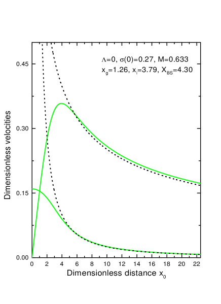
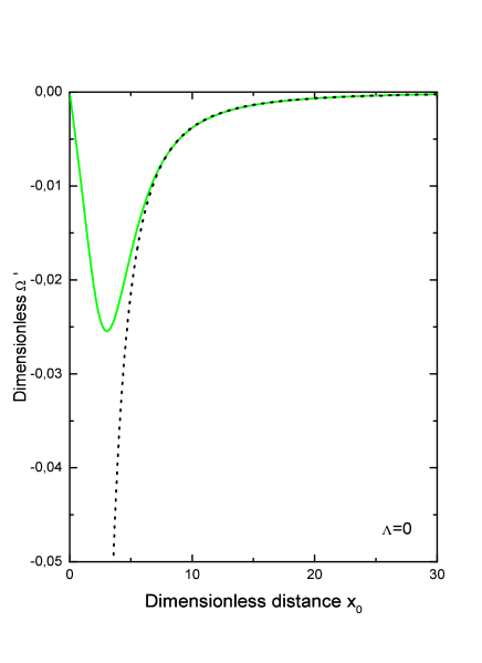
Figure 1: Left: Dimensionless velocities. The upper set of curves are $v_{\phi}$, the lower one are the rotational velocity $\Omega$, both for a boson star (solid) and a black hole (dash). The boson star has a dimensionless radius equal to $x_{BS}=4.3$, and a dimensionless mass equal to 0.633. The black hole has equal mass. Right: Dimensionless derivative of the rotational velocity, $\Omega^{\prime}$.

In Figure 1 we show the dimensionless rotational velocities, both $v_{\phi}$ and $\Omega$, for the previously quoted model. Through the comparison of the rotational velocities that a black hole of equal mass would produce, it is easy to see that a boson star is a highly relativistic object. The velocities for a black hole center are also shown in the Figure. A comparison of the power per unit area is shown in Figure 2. It is also shown there the difference between the temperatures of the disc. As one would expect from the behavior of the metric coefficients, the boson star curves, especially farther from the central object, tend to mimic those of the black hole case. However, in the inner parts of the disc, it is apparent that a slight deviation can be noticed. The boson star produce more power per unit area, and a hotter disc, than a black hole of equal mass. In order to see whether the dependence on the self-interaction parameter is strong, we have computed these same quantities for the case of $\Lambda=100$ and the same total mass and accretion rate. We have used a central density equal to $\sigma(0)=0.093$, what yields a boson star mass -in dimensionless units- equal to 2.25. In order for this dimensionless mass to rightfully represents the size of the central object, we need a boson mass equal to $1.20\times 10^{-25}$GeV.

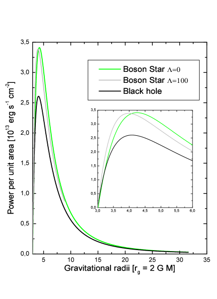
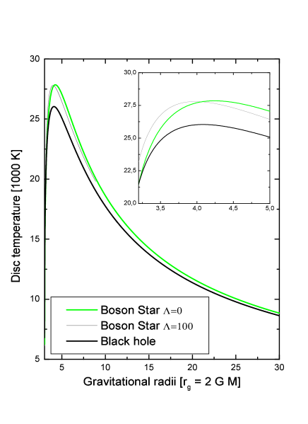
Figure 2: Left: Dimensionfull power per unit area for a black hole, and boson stars with self-interaction equal to 0 and to 100, all of the same mass. The position where the maximum of the curves are is zoomed out in the figure. Right: Dimensionfull temperatures of the disc for a black hole, and boson stars with self-interaction equal to 0 and to 100, all of the same mass. The position where the maximum of the curves are is zoomed out in the figure.

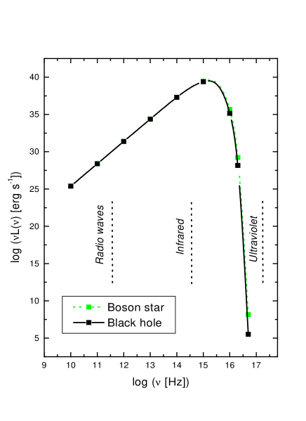
Figure 3: The final emission spectrum. Differences between the boson star cases with and without self-interaction are negligible, they are not noticed in the plot. Noticeable deviations between a supermassive black hole and a boson star begin at the far ultraviolet.

The final spectrum of the radiation emitted by the disc was computed and it is shown in Figure 3. It is clearly seen that throughout most parts of the electromagnetic spectrum, the obtained differences in the disc properties, such as the temperature or the power per unit area, will not be observationally noticed. Differences between the boson star cases with and without self-interaction are negligible. However, it appears that differences between black hole and boson stars centers turn out to be important at the most energetic part of the electromagnetic range, beginning in the far ultraviolet. The disc model we are considering does not produce energy in the X-ray and gamma-ray bands, but the possibility is open that even in the simplest non-relativistic case we have considered, a boson star and a black hole case could in principle be distinguished by the radiation properties at high energies. We can expect that better and more realistic models of accretion discs can show stronger differences.

The metric potentials of a boson star make the rotational velocities and their derivatives, except for the innermost parts of the disc, always greater than their counterparts produced by a central black hole. Looking at the left panel of Figure 1, it can be seen that only for the more central coordinates, the black hole rotational velocity is greater than that produced by a boson star. From the right panel we see, in addition, that the derivative of $\Omega$ is also always greater for a boson star than for a black hole. Recalling that $D(r)\propto\Omega\Omega^{\prime}$, a greater rotational velocity and rotational velocity gradient implies a greater power. The same happens for the temperature of the disc. The innermost part of Figure 1, where the rotational velocity of the particles rotating around a black hole diverges, can not be taken into account. These particles are all following unstable orbits and are not part of the disc, which begins at $x_{i}=3x_{g}$, at a value of about 4 in the x-axis of Figure 1. The effect of a larger temperature and power per unit area is then the integrated output of a disc rotating faster when a boson star is the central object.

Before ending this section we shall provide a brief discussion on the boson mass chosen. This discussion is based in our previous paper [3], as well as in [33]. As discussed in [3], based on the constraints imposed by the mass-radius relationship valid for the scalar stars analyzed, we may conclude that 1. if the boson mass is comparable to the expected Higgs mass (hundreds of GeV), then the center of the galaxy could be a non-topological soliton star [26], 2. an intermediate mass boson could produce a super-heavy object in the form of a boson star, and 3. for mini-boson stars to be used as central objects for galaxies the existence of an ultralight boson is needed. These conclusions are to considered as order of magnitude estimates. If boson stars really exist, they could be the remnants of first-order gravitational phase transitions and their mass should be ruled by the epoch when bosons decoupled from the cosmological background. The Higgs particle could be a natural candidate as constituent of a boson condensation if the phase transition occurred in early epochs. A boson condensation should be considered as a sort of topological defect relic. If soft phase-transitions took place during cosmological evolution e.g., soft inflationary events, the leading particles could have been intermediate mass bosons and so our super-massive objects should be genuine boson stars. If the phase transitions are very recent, the ultralight bosons could belong to the Goldstone sector giving rise to miniboson stars. We should also mention the possible dilatons appearing in low-energy unified theories, where the tensor field of gravity is accompanied by one or several scalar fields. In string effective supergravity, the mass of the dilaton can be related to the supersymmetry breaking scale $m_{SUSY}$ by $m_{\phi}\sim 10^{-3}(m_{SUSY}/TeV)^{2}$ eV. Finally, a scalar with a long history as a dark matter candidate is the axion, which has an expected light mass $m_{\sigma}\sim 7.4(10^{7}$ GeV$/f_{\sigma})$eV $\sim 10^{-11}$ eV with decay constant $f_{\sigma}$ close to the Planck mass.

4 Coordinate dependent Eddington luminosity

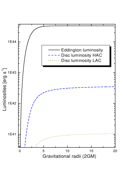
Figure 4: Comparison between the dimensionfull Eddington luminosity, now dependent on the radial coordinate, and the power radiated by the disc at different radius. HAC stands for a high accretion rate, here taken to be equal to $2\times 10^{-4}M_{\odot}$yr^-1. LAC stands for a low accretion rate, equal to $2\times 10^{-6}M_{\odot}$yr^-1. The coordinate dependent Eddington luminosity is everywhere greater than the power generated by a thin disc about a boson star. Note that the form of the curve for the Eddington luminosity is provided by that of the mass distribution within the boson star.

It is interesting to make now a comment on the Eddington luminosity ($L_{E}$) when a boson star is the central object. Consider first the basic concept. If the luminosity produced by the accreted material is too great, then the radiation pressure it would produce would blow up the infalling matter. The limiting luminosity, known as $L_{E}$, is found by balancing the inward force of gravity with the outward pressure of radiation [34]. This limit is then found by assuming that the infalling matter is fully ionized, and that the radiation pressure is provided by Thompson scattering of photons against electrons -which in turn are strongly coupled with the protons resident in the plasma by the electromagnetic interaction. Equating the involved forces results, in a first approximation, ${\sigma_{T}L}/{4\pi r^{2}c}={GMm_{p}}/{r^{2}},$ where $\sigma_{T}$ is the Thompson scattering cross section and $m_{p}$ is the proton mass. When this relationship is fulfilled, $L=L_{E}$. $L_{E}$ is the maximum luminosity which a spherically symmetric source of mass $M$ can emit in a steady state. Longair [35] provides the value of the Eddington luminosity in watts by introducing the gravitational radius $r_{g}$, $L_{E}={2\pi r_{g}m_{p}c^{3}}/{\sigma_{T}}=1.3\times 10^{31}{M}/{M_{\odot}}{\rm W}.$ None of the active galactic nuclei were found to exceed this limit [35]. It is interesting to note that if $M$ is constant, as in the case of a black hole, this limit is independent of the radius, that is, if $L<L_{E}$ at any given radius, the inequality will be sustained everywhere. A boson star -as well as any other transparent object- has a non-constant mass distribution and the Eddington luminosity become a coordinate dependent magnitude. In this situation, one may ask if there is any point within the stellar structure such that, even if $L<L_{E}$ outside the star, the opposite inequality is valid at this point. If this is so, and $L>L_{E}(r=r_{0})$, steady accretion would not proceed. We would so be able to define the internal border of the disc. $L_{E}(r)$ is given by the distribution of mass, since $L_{E}(r)\propto M(r)$. For the luminosity produced by the disc we have to integrate the power produced by a disc slab of size $dr$ from $r_{i}$ to $r$. This is what should be compared with $L_{E}(r)$. Then, we compute the total power radiated between $r_{i}$ and $r$ as

$$P=2\int_{r_{i}}^{r}D(r)2\pi rdr=-5.705\times 10^{46}\;\dot{M}[\frac{M_{\odot}}{{\rm yr}}]\;\frac{{\rm erg}}{{\rm s}^{-1}}\;\int_{r_{i}}^{r}\frac{1}{2}\;[\Omega]\;[\Omega^{\prime}]\;x^{2}dx.$$ (9)

In Figure 4, we show the results for the Eddington luminosity for a non self-interacting boson star, compared with the power radiated by the disc for two different accretion rates. In none of these cases, the power generated in circles whose radii are smaller than the star size overcomes $L_{E}$. This also supports the idea that accretion can continue inwards, within the boson star structure.

5 A relativistic treatment for the accretion

Even when useful as a first approach, the presented treatment fail when considering the innermost part of the disc, especially when the disc orbiting a boson star has a more internal commencement than that orbiting around a black hole. In order to get a complete picture, we have to treat the problem in a relativistic way, this is objective of the rest of this paper.

5.1 Particle orbits

Consider again the stationary, spherically symmetric, time independent, line element, written as

$$ds^{2}=-B(r)dt^{2}+\frac{1}{1-2M(r)/r}dr^{2}+r^{2}(d\theta^{2}+\sin^{2}\theta\,d\phi^{2})\;.$$ (10)

Again, the Schwarzschild solution is a special case of Eq. (10), occurring when $B(r)=1-2M(r)/r$ and $M(r)$ is a constant equal to the mass of the black hole. In our present situation, $B(r)$ must be consistent both with an asymptotically flat space-time and with the absence of a singularity. $M(r)$, in turn, decreases with decreasing radius, being equal to 0 at $r=0$. The particle orbits in that general metric will be determined by the conserved quantities, $E=-p_{t}:{\rm total\;energy}$; $L=p_{\theta}:{\rm component\;of\;the\;angular\;momentum.}$ An additional constant of motion will be the mass of the test particle, let us call it $\hat{m}$, which can be absorbed by redefining quantities in a per-unit-mass basis. The general (non-trivial) equations for the orbital trajectory in a space-time described by Eq. (10) are:

$$r^{2}\left[g_{rr}g_{tt}\right]^{1/2}\frac{dr}{d\lambda}=V(r)^{1/2}=\left[E^{2}r^{4}-r^{4}B\left(1+\frac{L^{2}}{r^{2}}\right)\right]^{1/2},$$ (11)

$$r^{2}\frac{d\phi}{d\lambda}=\frac{L}{\sin^{2}\theta}.$$ (12)

For a general derivation see the book by Weinberg [22] (take caution with the different definition of the symbols). Here, $\lambda$ is an affine parameter related with the proper time $\tau$, by $\lambda=\tau/\hat{m}$. We shall take $\hat{m}=1$ for massive particles. A prime will denote derivation with respect to $r$.

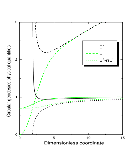
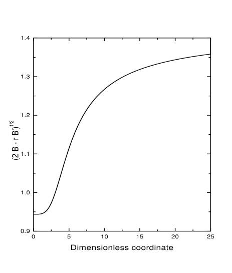
Figure 5: Left: Radial dependence of the energy, angular momentum, and the difference between them -with the momentum weighted by the rotational velocity $\Omega$- for circular geodesics, all per unit mass. The divergent curves are the corresponding magnitudes for the Schwarzschild black hole case. Right: Radial dependence of the denominator of the expressions for $E^{\dagger}$ and $L^{\dagger}$. Being the values it takes all positive, it is shown that it is possible to find a circular orbit even within the boson star. Details of the model are as follows: The mass for both, the black hole and the boson star, was taken as $M=0.633m_{\rm Pl}^{2}/m$, with $m$ the mass of the constituent bosons, a free parameter. The central density, in usual dimensionless units, is equal to 0.27. No self-interaction was considered. All figures in this Section are based on this same model, but the behavior is generic. The radial coordinate is $x=mr$.

We are interested in the circular orbits. For such class, $dr/d\lambda$ must vanish instantaneously and at all subsequent moments, what imposes the conditions, $V(r)=0\;\;\;{\rm and}\;\;\;V(r)^{\prime}=0.$ These equations determine $E$ and $L$, which per unit mass, are given by

$$\frac{E}{\hat{m}}=E^{\dagger}=\left(\frac{2B^{2}}{2B-rB^{\prime}}\right)^{1/2},\;\;\;\;\;\;\frac{L}{\hat{m}}=L^{\dagger}=\left(\frac{B^{\prime}r^{3}}{2B-rB^{\prime}}\right)^{1/2}.$$ (13)

These quantities are shown –both for the black hole and the boson star case– in the left panel of Figure 5. One can immediately show that both $E^{\dagger}$ and $L^{\dagger}$ reduce themselves to the Schwarzschild expressions when $B(r)=1-2M/r$, and that they tend to them asymptotically. Circular orbits might not exist for all values of $r$. It is needed that the denominator of $E^{\dagger}$ and $L^{\dagger}$, be well-defined, i.e. $2B-rB^{\prime}>0$. But in the case of a boson star, this happens for all values of the radial coordinate, see the right panel of Figure 5. Then, in a relativistic non-baryonic potential, generated by a non-rotating compact object, there are circular orbits for every possible value of the radial coordinate, including those which are inside the structure. It is interesting to note, in addition, that $E^{\dagger}<1$, so there are no unbound orbits, hyperbolic in energetics [36].

The circular orbits might not all be stable. Stability requires that, when evaluated using the general expressions given in Eq (13), $V(r)^{\prime\prime}\leq 0$. This yields

$$V(r)^{\prime\prime}(2B-rB^{\prime})=-6BB^{\prime}r^{3}+4(B^{\prime})^{2}r^{4}-2BB^{\prime\prime}r^{4}\leq 0.$$ (14)

Again, this reduces to the Schwarzschild case when $B(r)=1-2M/r$. The results of this computation in a generic boson star potential are shown in the left panel of Figure 6. For all values of $r$, $V(r)^{\prime\prime}\leq 0$. Then, in a relativistic non-baryonic potential, generated by a non-rotating compact object, all circular orbits, even those within the structure, are stable.

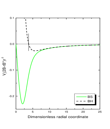
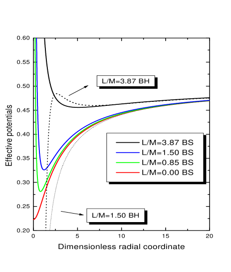
Figure 6: Left: Radial dependence of the second derivative of $V(r)$, both for a Schwarzschild black hole (dash line) and a boson star (solid line). The minimum radius at which a stable orbit exists in the black hole case is $r=6M$, it is marked with a crossing in the plot. For the boson star, all circular orbits are stable. Right: Effective potential for different values of $L/M$, with $M$ the dimensionless total mass of the star, as in Figure 5. Two cases of the black hole effective potential are shown for comparison. BS(H) stands for boson star (black hole). The $x$-axis is the $z$ variable, introduced in the text. For the case of a black hole, $z$ and $x$ coincide.

5.2 From relativistic orbits to relativistic spectrum

The power per unit area generated in a disc rotating around a compact central object, which produces a relativistic potential, is given by [37]

$$D(r) = \frac{\dot{M}}{4\pi}\frac{1}{r}\left[B\left(1-\frac{2M}{r}\right)\right]^{1/2}\left(-\frac{d\Omega}{dr}\right)\left(E^{\dagger}-\Omega L^{\dagger}\right)^{-2}\int_{r_{ms}}^{r}\left(E^{\dagger}-\Omega L^{\dagger}\right)\left(\frac{dL^{\dagger}}{dr}\right)dr=$$ (17)

$$1.4706\times 10^{74}\frac{{\rm erg}}{{\rm cm}^{2}{\rm s}}m^{2}[{\rm GeV}]\frac{\dot{M}[M_{\odot}{\rm yr}^{-1}]}{4\pi}\times\hskip 227.62204pt$$

$$\frac{1}{x}\left[B(x)\left(1-\frac{2M(x)}{x}\right)\right]^{1/2}\left(-\frac{d\Omega}{dx}\right)\left(E^{\dagger}-\Omega L^{\dagger}\right)^{-2}\int_{x_{ms}}^{x}\left(E^{\dagger}-\Omega L^{\dagger}\right)\left(\frac{dL^{\dagger}}{dr}\right)dx.$$

All physical quantities are to be used in dimensionless form (e.g. $B\longrightarrow B(x)$), and are explicitly given by

$$E^{\dagger}=\left(\frac{2B^{2}}{2B-xB^{\prime}}\right)^{1/2},\hskip 85.35826pt\Omega L^{\dagger}=\left(\frac{xB^{\prime}}{2(2B-xB^{\prime})}\right)^{1/2}.$$ (18)

Clearly, when comparing with the output produced by a disc rotating upon a central black hole, $D(r)$ will change not only because of the modifications in $\Omega$, $E^{\dagger}$, and $L^{\dagger}$, but also because of the change in the integration limits. Here, $r_{ms}$ is the position of the innermost stable circular geodesic orbit. Using the latter expression and all obtained results for other physical parameters of the particle orbits, we can get the relativistic results we were searching.

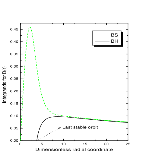
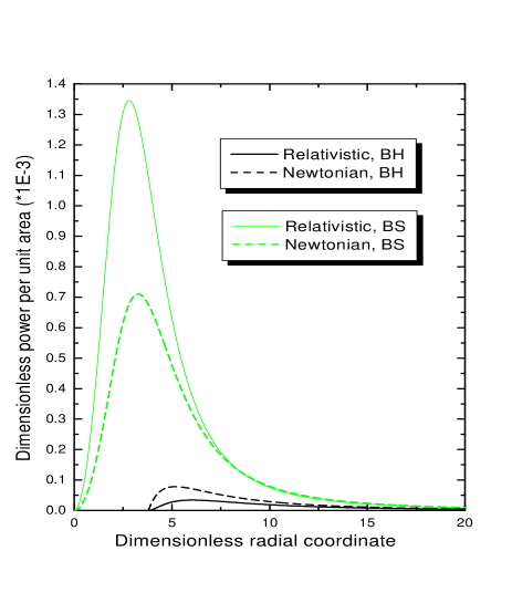
Figure 7: Left: Integrands for D(r), both for a black hole and a boson star of the same mass. The BH last stable orbit is marked. Right: Relativistic power per unit area. In dash lines, we show, for comparison, also the Newtonian results for both cases.

Figure 7 shows the results of some crucial intermediate computation needed to get the relativistic spectrum, and, on the right panel, the power per unit area in the relativistic disc. It can be seen there that there is an interesting effect produced by boson stars as central objects: While a relativistic treatment of the disc reduces the expected emission from the innermost parts of a disc rotating around a Schwarzschild black hole, it dramatically enhances the expected one when a boson star is in the scenario. This has the consequence of a hardening in the emission spectrum, which is shown in Figure 8. The deviations shown between the spectra are impressive. Table 3 shows some of the values used to construct this latter figure.

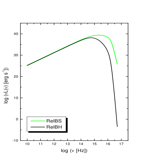
Figure 8: Relativistic emission spectrum for an accretion disc rotating around a static boson star. The black hole case is shown for comparison.

Table 1: Comparison of relativistic spectra.

$\nu$ [1/s]	$\nu L(\nu)$ [erg s-1]	$\nu L(\nu)$ [erg s-1]
	BS	BH
1010	$2.00\times 10^{25}$	$1.41\times 10^{25}$
1012	$2.00\times 10^{31}$	$1.41\times 10^{31}$
1014	$1.77\times 10^{37}$	$1.18\times 10^{37}$
1016	$1.36\times 10^{39}$	$3.46\times 10^{33}$

6 Conclusions

In this paper we have modeled a very simple accretion disc rotating around a static supermassive boson star, although we have given the scaling property that shows how to extend these results to other mass domains (equivalently, to other single boson mass cases). The disc was assumed steady, with a constant accretion rate, and thin, so that the standard theory can be applied. Throughout the paper, we have made a comparison of all results with those obtained for discs rotating around Schwarzschild black holes of the same mass. Our aim was to see whether the emissivity properties of the accretion disc are noticeably changed when the central object is. More complicated models for the accretion process as well as more realistic models for the star (as those in which the star is rotating) can be considered. We hope this work will encourage further analysis.

Acknowledgments

This work has been partially supported by CONICET and Fundación Antorchas. The author is on leave from IAR, and acknowledges an anonymous Referee for his remarks.

References

- [1] I. Tkachev, Soviet Astron. Lett. 12, 305 (1986); Phys. Lett. B191, 41 (1987); Phys. Lett. B261, 289 (1991).
- [2] D. Tsikaluri and R. D. Viollier, Astrophys. J. 500, 591 (1998); Astropart. Phys. 122, 199 (1999).
- [3] D. F. Torres, S. Capozziello, and G. Lambiase, Phys. Rev. D62, 104012 (2000).
- [4] A. M. Ghez, B. L. Klein, M. Morris, and E. E. Becklin, Astrophys. J. 509, 678 (1998); R. Genzel, N. Thatte, A. Krabbe, H. Kroker, and L. E. Tacconi-Garman, Astrophys. J. 472, 153 (1996); A. Eckart and R. Genzel, Nature 383, 415 (1996); Mon. Not. R. Astron. Soc. 284, 576 (1997).
- [5] J. Kormendy, and D. Richstone, ARA&A 33, 581 (1995).
- [6] Constellation X satellite web page: http://constellation.gsfc.nasa.gov/
- [7] Maxim satellite web page: http://maxim.gsfc.nasa.gov/
- [8] H. Falcke, F. Melia, and E. Agol, Astrophys. J. Lett. 528, 13 (2000).
- [9] E. W. Mielke and F. E. Schunck, Nucl.Phys. B564, 185 (2000)
- [10] F. E. Schunck and A. R. Liddle, Phys. Lett. B404, 25 (1997).
- [11] F. E. Schunck and D. F. Torres, Int. J. of Mod. Phys. D9, 601 (2000).
- [12] S. Capozziello, G. Lambiase, and D. F. Torres, Class. Quantum Grav. 17, 3171 (2000).
- [13] A. Iwazaki, Phys.Lett. B455, 192 (1999).
- [14] M. P. Dabrowski and F. E. Schunck, Astrophys. J.
- [15] K. S. Virbhadra, D. Narasimha, and S. M. Chitre, A & A, 337, 1 (1998); K. S. Virbhadra, and G. F. R. Ellis, A & A, astro-ph/9904193 (1999); D. F. Torres, G. E. Romero, and L. A. Anchordoqui, Phys. Rev D58, 123001 (1998), ibid. Mod. Phys. Lett. A13, 1575 (1998); M. Safonova, D. F. Torres, and G. E. Romero, Phys. Rev. D65, 023001 (2002), gr-qc/0105070; ibid. Mod. Phys. Lett. A16, 153 (2001); E. F. Eiroa, G. E. Romero, and D. F. Torres, Mod. Phys. Lett. A16, 973 (2001).
- [16] F. Ryan, Phys. Rev. D55, 6081 (1997).
- [17] A.B. Henriques, A. R. Liddle, R.G. Moorhouse, Nucl.Phys. B337, 737,1990
- [18] E. Seidel, and W. Suen, Phys. Rev. D42, 384 (1990).
- [19] F. V. Kusmartsev, E. W. Mielke, and F. E. Schunck, Phys. Rev. D43, 3895 (1991); Phys. Lett. A157, 465 (1991).
- [20] M. Heusler, Class. Quantum Grav. 12, 779 (1995).
- [21] F. E. Schunck, and E. W. Mielke Phys. Lett. A 249, 389 (1998).
- [22] S. Weinberg, Gravitation and cosmology (J. Wiley & Sons, New York, 1972).
- [23] U. Nucamendi, M. Salgado, and D. Sudarsky, Phys. Rev. D63, 125016
- [24] T. D. Lee and Y. Pang, Phys. Rep. 221, 251 (1992); A. R. Liddle and M. S. Madsen, Int. J. Mod. Phys. D1, 101 (1992); E. W. Mielke and F. E. Schunck: “Boson stars: Early history and recent prospects”, Proceedings of the 8th Marcel Grossmann meeting in Jerusalem, (World Scientific Publ., Singapore 1999, p.1607), gr-qc/9801063.
- [25] M. Colpi, S. L. Shapiro, and I. Wasserman, Phys. Rev. Lett. 57, 2485 (1986).
- [26] T. D. Lee, Phys. Rev. D35, 3637 (1987); R. Friedberg, T. D. Lee, and Y. Pang, Phys. Rev. D35, 3640, 3658, 3678 (1987).
- [27] D. F. Torres, Phys. Rev. D56, 3478 (1997); D. F. Torres, A. R. Liddle, and F. E. Schunck, Phys. Rev. D57, 4821 (1998); D. F. Torres, F. E. Schunck, and A. R. Liddle, Class. Quantum Grav. 15, 3701 (1998).
- [28] R. Ruffini and S. Bonazzola, Phys. Rev. 187, 1767 (1969).
- [29] D. J. Kaup, Phys. Rev. 172, 1331 (1968).
- [30] F. E. Schunck, and E. W. Mielke, in Proceedings of the Bad Honnef Workshop, Relativity and Scientific Computing: Computer Algebra, Numerics, Visualization, ed. F.W. Hehl, R.A. Puntigam, and H. Ruder (Berlin, Springer–Verlag, p.8 and 138, 1996); S. Yoshida, and Y. Eriguchi, Phys. Rev. D56, 762 (1997).
- [31] R. Narayan, R. Mahadevan, J. F. Grindlay, R. G. Popham, and C. Gammie, Astrophys. J. 492, 554 (1998).
- [32] R. Narayan, I. Yi, and R. Mahadevan, Nature 374, 623 (1995).
- [33] E. Mielke, and F. E. Schunck, Gen. Rel. Grav. 33, 805 (2001).
- [34] J. Frank, A. King and D. Raine, Accretion power in astrophysics (Cambridge University Press, Cambridge, 1995).
- [35] M. S. Longair, High energy astrophysics, Vol. II (Cambridge University Press, Cambridge, 1994).
- [36] J. M. Bardeen, W. H. Press, and S. A. Teulkolsky, ApJ 178, 347 (1972).
- [37] D. Page, and K. S. Thorne, ApJ 191, 499 (1974).