Status of the CKM matrix

Abstract

An updated determination of the parameters of the Cabibbo-Kobayashi-Maskawa matrix is presented.

1 Introduction

In the Standard Model, weak interactions of quarks are governed by the four parameters of the CKM matrix [1] which, in the Wolfenstein-Buras parametrisation [2, 3], are labelled as $\lambda,~{}A,~{}\bar{\rho}~{}{\rm and}~{}\bar{\eta}$. Measurements of semileptonic decays of strange and beauty particles are the main sources of information on $\lambda$ and $A$, respectively. The values of $\left|\varepsilon_{K}\right|$, $\left|V_{ub}/V_{cb}\right|$, $\Delta m_{d}$ and ${\Delta m_{s}}$ provide a set of four constraints for $\bar{\rho}$ and $\bar{\eta}$. These constraints depend, in addition, on other quantities obtained from measurements and/or theoretical calculations. The regions of $\bar{\rho}$ and $\bar{\eta}$ preferred by the four constraints are expected to overlap, as long as the Standard Model gives an overall description of the various experimental observations. In this paper, we summarize the results of our analysis of the CKM matrix. Further details on various aspects of this analysis can be found in ref. [4].

2 Basic Formulae

Four measurements restrict, at present, the possible range of variations of the $\bar{\rho}$ and $\bar{\eta}$ parameters:

• The relative rate of charmed and charmless $b$-hadron semileptonic decays which allows to measure the ratio

  $$\left|\frac{V_{ub}}{V_{cb}}\right|=\frac{\lambda}{1~{}-~{}\frac{\lambda^{2}}{2}}\sqrt{\bar{\rho}^{2}+\bar{\eta}^{2}}\,.$$ (1)

  .

• The ${B}^{0}_{d}-\bar{{B}}^{0}_{d}$ time oscillation period which can be related to the mass difference between the light and heavy mass eigenstates of the ${B}^{0}_{d}-\bar{{B}}^{0}_{d}$ system

  $$\Delta m_{d}\ = \ {G_{F}^{2}\over 6\pi^{2}}m_{W}^{2}\ \eta_{c}S(x_{t})\ A^{2}\lambda^{6}\ [(1-$$ (2)

  $$\bar{\rho})^{2}+\bar{\eta}^{2}]\ m_{B_{d}}\ f_{B_{d}}^{2}\hat{B}_{B_{d}}\ ,$$

  where $S(x_{t})$ is the Inami-Lim function [5] and $x_{t}=m_{t}^{2}/M^{2}_{W}$. $m_{t}$ is the $\overline{MS}$ top mass, $m_{t}^{\overline{MS}}(m_{t}^{\overline{MS}})$, and $\eta_{c}$ is the perturbative QCD short-distance NLO correction. The remaining factor, $f_{B_{d}}^{2}\hat{B}_{B_{d}}$, encodes the information of non-perturbative QCD. Apart for $\bar{\rho}$ and $\bar{\eta}$, the most uncertain parameter in this expression is $f_{B_{d}}\sqrt{\hat{B}_{B_{d}}}$. The value of $\eta_{c}=0.55\pm 0.01$ has been obtained in [6] and we used $m_{t}=(167\pm 5)\,\rm{GeV}$, as deduced from measurements of the mass by CDF and D0 Collaborations [7].

• The limit on the lower value for the time oscillation period of the ${B}^{0}_{s}-\bar{{B}}^{0}_{s}$ system is transformed into a limit on $\Delta m_{s}$ and compared with $\Delta m_{d}$

  $$\frac{\Delta m_{d}}{\Delta m_{s}} = \frac{m_{B_{d}}f_{B_{d}}^{2}\hat{B}_{B_{d}}}{m_{B_{s}}f_{B_{s}}^{2}\hat{B}_{B_{s}}}\ \left(\frac{\lambda}{1-\frac{\lambda^{2}}{2}}\right)^{2}\times$$ (3)

  $$[(1-\bar{\rho})^{2}+\bar{\eta}^{2}]\,.$$

  The ratio $\xi~{}=~{}f_{B_{s}}\sqrt{\hat{B}_{B_{s}}}/f_{B_{d}}\sqrt{\hat{B}_{B_{d}}}$ is expected to be better determined from theory than the individual quantities entering into its expression. In our analysis, we accounted for the correlation due to the appearance of $\Delta m_{d}$ in both Equations (2) and (3).

• CP violation in the kaon system which is expressed by $\left|\varepsilon_{K}\right|$

  $$\left|\varepsilon_{K}\right|\ = C_{\varepsilon}\ A^{2}\lambda^{6}\ \bar{\eta}\Big{[}-\eta_{1}S(x_{c})+$$ (4)

  $$\eta_{2}S(x_{t})\left(A^{2}\lambda^{4}\left(1-\bar{\rho}\right)\right)+$$

  $$\eta_{3}S(x_{c},x_{t})\Big{]}\ \hat{B}_{K}\ ,$$

  where

  $$C_{\varepsilon}=\frac{G_{F}^{2}f_{K}^{2}m_{K}m_{W}^{2}}{6\sqrt{2}\pi^{2}\Delta m_{K}}\ .$$ (5)

  $S(x_{i})$ and $S(x_{i},x_{j})$ are the appropriate Inami-Lim functions [5] of $x_{q}=m_{q}^{2}/m_{W}^{2}$, including the next-to-leading order QCD corrections [6, 8]. The most uncertain parameter is $\hat{B}_{K}$.

Constraints are obtained by comparing present measurements with theoretical expectations using the expressions given above and taking into account the different sources of uncertainties. In addition to $\bar{\rho}$ and $\bar{\eta}$, these expressions depend on other quantities which have been listed in Table 1. Additional measurements or theoretical determinations have been used to provide information on the values of these parameters.

Table 1: Values of the quantities entering into the expressions of $\left|\varepsilon_{K}\right|$, $\left|V_{ub}/V_{cb}\right|$, $\Delta m_{d}$ and $\Delta m_{s}$. In the third and fourth columns the Gaussian and the flat part of the uncertainty are given, respectively.

Parameter	Value	Gaussian	Uniform	Ref.
		$\sigma$	half-width
$\lambda$	$0.2237$	$0.0033$		[4]
$\left|V_{cb}\right|$	$40.7\times 10^{-3}$	$1.9\times 10^{-3}$		[4]
$\left|V_{ub}\right|$	$36.1\times 10^{-4}$	$4.6\times 10^{-4}$	–	[4]
$\left|\varepsilon_{K}\right|$	$2.271\times 10^{-3}$	$0.017\times 10^{-3}$	–	[9]
$\Delta m_{d}$	$0.489~{}\mbox{ps}^{-1}$	$0.008~{}\mbox{ps}^{-1}$	–	[10]
$\Delta m_{s}$	$>$ 14.6 ps-1 at 95% C.L.	see text		[10]
$m_{t}$	$167~{}\rm{GeV}$	$5~{}\rm{GeV}$	–	[7]
$m_{b}$	$4.23~{}\rm{GeV}$	$0.07~{}\rm{GeV}$	–	[11]
$m_{c}$	$1.3~{}\rm{GeV}$	$0.1~{}\rm{GeV}$	–	[9]
$\hat{B}_{K}$	$0.87$	$0.06$	$0.13$	[4]
$f_{B_{d}}\sqrt{\hat{B}_{B_{d}}}$	$230~{}\rm MeV$	$25~{}\rm MeV$	$20~{}\rm MeV$	[4]
$\xi=\frac{f_{B_{s}}\sqrt{\hat{B}_{B_{s}}}}{f_{B_{d}}\sqrt{\hat{B}_{B_{d}}}}$	$1.14$	0.04	$0.05$	[4]
$\alpha_{s}$	$0.119$	$0.003$	–	[8]
$\eta_{1}$	$1.38$	$0.53$	–	[8]
$\eta_{2}$	$0.574$	$0.004$	–	[6]
$\eta_{3}$	$0.47$	$0.04$	–	[8]
$\eta_{b}$	$0.55$	$0.01$	–	[6]
$f_{K}$	$0.159~{}\rm{GeV}$	fixed		[9]
$\Delta m_{K}$	$0.5301\times 10^{-2}~{}\mbox{ps}^{-1}$	fixed		[9]
$G_{F}$	$1.16639\times 10^{-5}~{}\rm{GeV}^{-2}$	fixed		[9]
$m_{W}$	$80.42~{}\rm{GeV}$	fixed		[9]
$m_{B^{0}_{d}}$	$5.2792~{}\rm{GeV}$	fixed		[9]
$m_{B^{0}_{s}}$	$5.3693~{}\rm{GeV}$	fixed		[9]
$m_{K}$	$0.493677~{}\rm{GeV}$	fixed		[9]

3 Inferential framework

The phenomenological analysis is performed using the Bayesian inference. In this framework, every parameter entering the constraints, regardless their theoretical or experimental origin, is characterized by a probability density function (p.d.f.). We assign the p.d.f.s of the different parameters as shown in Table 1. These distributions are taken as Gaussian or flat or a convolution of the two, according to the origin of the uncertainty being purely statistical or coming from influence quantities (such as theoretical parameters or systematic errors in experiments). The parameters $\bar{\rho}$ and $\bar{\eta}$ have also an a-priori p.d.f. which is assumed to be flat. Using these distributions and the experimental constraints discussed in the previous section, we can build an overall likelihood and obtain a-posteriori p.d.f.s for $\bar{\rho}$ and $\bar{\eta}$ or any other quantities of interest.

This method provides a theoretically-sound approach that allows a consistent treatment of the systematic and theoretical uncertainties and makes it possible to define regions where the values of $\bar{\rho}$ and $\bar{\eta}$ (as well as of other quantities) are contained with any given level of probability.

The Bayesian method applied to the CKM-matrix analysis is discussed at length in ref. [4].

A different analysis based on frequentistic techniques can be found in ref. [12]. This paper also puts forth a rather academic argument that, in the mind of its authors, should demonstrate that the Bayesian method unfairly narrows the region of predicted results for quantities depending on more than one theoretical parameter. The argument is the following: consider a quantity $T_{P}=x_{1}x_{2}x_{3}\dots x_{N}$, defined as the product of $N$ “theoretical” parameters $x_{i}$, and assume to know that these parameters lie in the range $[-1,1]$. Following the Bayesian method one easily finds that the resulting p.d.f. of $T_{P}$ peaks at zero and becomes more and more peaked as the number $N$ of parameters increases. This leads the authors of refs. [12, 13] to conclude that the Bayesian method is “dangerous”, since a safe method should have predicted $T_{P}$ in the range $[-1,1]$. However, our conclusion is quite the opposite. It is perfectly natural that the p.d.f. of $T_{P}$ peaks as $N$ increases, being simply the effect of combinatorics (unless, of course, there are reasons to believe that the different determinations of the $x_{i}$ are correlated). The singularity of the p.d.f. as $N$ goes to infinity, which has been pointed out as a pathology of the Bayesian method, has also a simple explanation: the knowledge of an infinite number of p.d.f. for the $x_{i}$ corresponds to determining $T_{P}$ with infinite precision. Therefore we believe that the argument presented in ref. [12] does not affect the validity of the Bayesian method in any way. We rather find that methods which predict $T_{P}$ in the range $[-1,1]$ are deliberately throwing away information. This may be justified and reasonable in specific and well-motivated cases, but as a general rule, we find it quite contrary to the spirit of this kind of analyses aiming to use present theoretical and experimental information to extract the best determination of the unitarity triangle in the Standard Model.

Figure 1: The likelihood ratio ${\rm R}(\Delta m_{s})$ used in the analysis.

4 Input Parameters

The values of the input parameters used in the anaysis are collected in Table 1. For all the theoretical parameters, we have used results taken from lattice QCD. There are several reasons for this choice, which has been adopted also in previous studies of the unitarity triangle [14, 15, 16, 17, 18]. Lattice QCD is not a model, as the quark model for example, and therefore physical quantities can be computed from first principles without arbitrary assumptions. It provides a method for predicting all physical quantities (decay constants, weak amplitudes, form factors) within a unique, coherent theoretical framework. For many quantities the statistical errors have been reduced to the percent level. Although most of the results are affected by systematic effects, the latter can be “systematically” studied and eventually corrected. All the recent literature on lattice calculations is indeed focused on discussions of the systematic errors and studies intended to reduce these sources of uncertainty. Finally, in cases where predictions from lattice QCD have been compared with experiments, for example $f_{D_{s}}$, the agreement has been found very good. Obviously, for some quantities the uncertainty from lattice simulations is far from being satisfactory and further effort is needed to improve the situation. Nevertheless, for the reasons mentioned before, we think that lattice results and uncertainties are the most reliable ones and we have used them in our study.

Results from the LEP working groups have been used for $\Delta m_{d}$ and $\Delta m_{s}$. LEP and CLEO measurements of $\left|{V}_{cb}\right|$ and $\left|{V}_{ub}\right|$ have been combined to obtain the values in Table 1. Details on the methods used for combining the various measurements can be found in [4]. In order to include the information from the lower limit on $\Delta m_{s}$ in the analysis, we have found it better to use the likelihood ratio R defined as

$${\rm R}(\Delta m_{s})=e^{\textstyle{-\Delta\log{\cal L}^{\infty}(\Delta m_{s})}}=\frac{{\cal L}(\Delta m_{s})}{{\cal L}(\infty)}\ ,$$ (6)

with

$$\Delta\log{\cal L}^{\infty}(\Delta m_{s}) = \frac{\textstyle 1}{\textstyle 2}\,\left[\left(\frac{\textstyle{\cal A}-1}{\textstyle\sigma_{\cal A}}\right)^{2}-\left(\frac{\textstyle{\cal A}}{\textstyle\sigma_{\cal A}}\right)^{2}\right]$$ (7)

$$= \left(\frac{\textstyle 1}{\textstyle 2}-{\cal A}\right){\textstyle 1\over\textstyle\sigma_{\cal A}^{2}}\ ,$$

where ${\cal A}$ is the measured oscillation amplitude at a given value of $\Delta m_{s}$, expected to be equal to one at the physical $\Delta m_{s}$ and to vanish elsewhere. The likelihood ratio is more effective than the usual likelihood as it exploits the fact that the oscillation is signaled by the amplitude being both compatible with one and incompatible with zero. A thorough discussion of this method is presented in [4]. The likelihood ratio R used in the analysis is shown in Figure 1.

Figure 2: Contour plots in the ($\bar{\rho}$,$\bar{\eta}$) plane.

5 Results

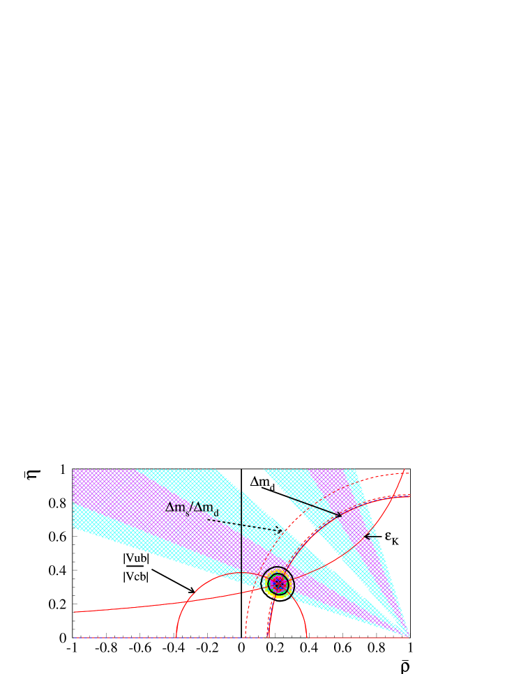
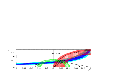
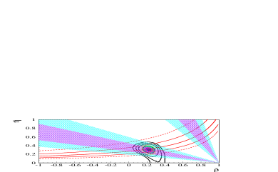
The region in the ($\bar{\rho},~{}\bar{\eta})$ plane selected by the measurements of $\left|\varepsilon_{K}\right|$, $\left|V_{ub}/V_{cb}\right|$, $\Delta m_{d}$ and from the information on $\Delta m_{s}$ (using the R function in Figure 1) is given in the upper part of Figure 2. On the lower-left part, the uncertainty bands for the quantities, obtained using Equations (1)–(4), are presented. Each band, corresponding to only one of the constraints, contains 68% and 95% of the events obtained by varying the input parameters. This comparison illustrates the consistency of the different constraints provided by the Standard Model. The measured values of $\bar{\rho}$ and $\bar{\eta}$ are

$$\bar{\rho}=0.218\pm 0.038,~{}\bar{\eta}=0.316\pm 0.040$$ (8)

The two quantities are practically uncorrelated (correlation coefficient of -5%), as it can be seen from the contour plots in the ($\bar{\rho},~{}\bar{\eta})$ plane. Fitted values for the angles of the unitarity triangle have been also obtained

$$\!\!\!\!\!\sin(2\,\beta)=0.696\pm 0.068\,,~{}\gamma=(55.5\pm 6.2)^{\circ}\,,$$

$$\!\!\!\!\!\sin(2\,\alpha)=-0.42\pm 0.24\,.$$ (9)

Figure 3: Some a-posteriori p.d.f.

In Figure 3, the p.d.f. for the angles of the unitarity triangle are given. Few comments can be made:

• $\sin(2\beta)$ is determined quite accurately. This value has to be compared with the world average $\sin(2\beta)=0.79\pm 0.10$ [19];

• the angle $\gamma$ is known within an accuracy of about 10%. It has to be stressed that, with present measurements, the probability that $\gamma$ is greater than 90^∘ is only 0.03%. Without including the information from $\Delta m_{s}$, it is found that $\gamma$ has 4% probability to be larger than 90^∘.

As four constraints are used to determine the values of two parameters, it is possible to relax, in turn, one (or more) of these constraints, still obtaining significant confidence intervals. An interesting exercise consists in removing the theoretical constraint for $\hat{B}_{K}$ in the measurement of $\left|\varepsilon_{K}\right|$ ([20]-[21]). The corresponding selected region in the ($\bar{\rho},~{}\bar{\eta})$ plane is shown in lower-right plot of Figure 2, where the region selected by the measurement of $\left|\varepsilon_{K}\right|$ alone is also drawn. This comparison shows that the Standard Model picture of CP violation in the $K$ system and of $B$ decays and oscillations are consistent. In the same figure, we also compare the allowed regions in the ($\bar{\rho},~{}\bar{\eta})$ plane with those selected by the measurement of $\sin(2\,\beta)$ using $J/\psi K_{S}$ events.

Using constraints from $b$-physics alone the following results are obtained

$$\begin{array}[]{ll}\bar{\eta}=0.304^{+0.050}_{-0.058},&\\ \qquad 0.167\leq\bar{\eta}\leq 0.400&\rm{at}~{}95\%~{}{\rm prob.}\\ \sin(2\,\beta)=0.676^{+0.078}_{-0.096},&\\ \qquad 0.430\leq\sin(2\,\beta)\leq 0.820&\rm{at}~{}95\%~{}{\rm prob.}\\ \end{array}$$ (10)

Another way for illustrating the agreement between $K$ and $B$ measurements consists in comparing the values of the $\hat{B}_{K}$ parameter obtained in lattice QCD calculations with the value extracted from Equation (4), using the values of $\bar{\rho}$ and $\bar{\eta}$ selected by $b$-physics alone

$$\hat{B}_{K}^{\rm b-phys}=0.88^{+0.27}_{-0.13},$$

$$0.65\leq\hat{B}_{K}^{\rm b-phys}\leq 1.65~{}{\rm at}~{}95\%~{}{\rm prob.}$$ (11)

Since $\hat{B}_{K}$ is not limited from above, for the present study, probabilities are normalised assuming $\hat{B}_{K}<$5.

The importance of $B^{0}_{s}$–$\bar{B}^{0}_{s}$ mixing can be illustrated from the p.d.f. of the angle $\gamma$ obtained with or without including the $\Delta m_{s}$ constraint (respectively light and dark lines in the lower-left plot of Figure 3). High values for $\gamma$ are excluded at high confidence level by the experimental lower limit on $\Delta m_{s}$.

It is also possible to extract the probability distribution for $\Delta m_{s}$, from which one obtains

$$\Delta m_{s}=(16.1\pm 3.2)\ {\rm ps}^{-1}\,,$$

$$9.4\leq\Delta m_{s}\leq 23.0~{}{\rm ps}^{-1}~{}{\rm at}~{}95\%\ {\rm prob.}$$ (12)

If the information from the ${B}^{0}_{s}-\bar{{B}}^{0}_{s}$ analyses is included, results become

$$\Delta m_{s}=(17.1^{+1.5}_{-0.9})\ {\rm ps}^{-1}\,,$$

$$15.4\leq\Delta m_{s}\leq 20.3~{}{\rm ps}^{-1}~{}{\rm at}~{}95\%\ {\rm prob.}$$ (13)

These values are in agreement with the recent estimate of $\Delta m_{s}=15.8(2.3)(3.3)\ ps^{-1}$, presented in [23].

The value of $f_{B_{d}}\sqrt{\hat{B}_{B_{d}}}$ can be obtained by removing the theoretical constraint coming from this parameter in ${B}^{0}_{d}$–$\bar{B}^{0}_{d}$ oscillations. Using the two other theoretical inputs, $\hat{B}_{K}$ and $\xi$, $f_{B_{d}}\sqrt{\hat{B}_{B_{d}}}$ is measured with an accuracy which is better than the current evaluation from lattice QCD, given in Table 1. We obtain

$$f_{B_{d}}\sqrt{\hat{B}_{B_{d}}}=(228\pm 12)\,\rm MeV\,.$$ (14)

The present analysis shows that these results are in practice very weakly dependent on the exact value taken for the uncertainty on $f_{B_{d}}\sqrt{\hat{B}_{B_{d}}}$. An evaluation of this effect has been already presented in [24] where the flat part of the theoretical uncertainties on $f_{B_{d}}\sqrt{\hat{B}_{B_{d}}}$ was multiplied by two. Similar tests will be shown in Section 6.

It is even possible to remove the theoretical constraints on both $f_{B_{d}}\sqrt{\hat{B}_{B_{d}}}$ and $\hat{B}_{K}$ and obtain the simultaneous lower bound

$$\hat{B}_{K}>0.5\,~{}~{}{\rm and}~{}~{}f_{B_{d}}\sqrt{\hat{B}_{B_{d}}}>150\,\,\mbox{MeV}$$ (15)

at $95\%$ probability.

6 Stability of the results

The sensitivity of present results on the assumed probability distributions attached to the input parameters was studied. The comparison of the results obtained by varying the size of the theoretical uncertainties has been done to evaluate the sensitivity to these variations of uncertainties quoted on fitted values. This must not be taken as a proposal to inflate the uncertainties obtained in the present analysis.

In these tests, all values for uncertainties of theoretical origin have been, in turn, multiplied by two. For the quantities $\left|{V}_{ub}\right|$ and $\left|{V}_{cb}\right|$, new p.d.f. have been determined, following the prescriptions mentioned in Section 4 and used in the analysis. The main conclusion of this exercise is that, even in the case where all theoretical uncertainties are doubled, the unitarity triangle parameters are determined with an uncertainty which increases only by about 1.5.

Figure 4: Dependence of $\gamma$ on the maximum value of the phenomenological parameter $|\rho_{A}|$ appearing in the model used to compute $BR(B\to K\pi,\pi\pi)$. The bands correspond to $1\sigma$ ranges.

7 CKM angle $\gamma$ from $B\to K\pi,\pi\pi$ decays

It has been recently suggested that it is possible either to extract the CKM angle $\gamma$ using the measured $BR$s of $B\to K\pi,\pi\pi$ decays or, at least, use this experimental information to improve the results of the unitarity triangle analysis [25]. Although in principle this is certainly true, in practice it requires a very good control on the hadronic uncertainties entering the theoretical predictions of these $BR$s. Contrary to recent claims, however, the theoretical progresses in understanding in the infinite mass limit factorization of hadronic matrix elements do not help in the specific case. In fact, $B\to K\pi,\pi\pi$ channels get large, if not dominant, contributions from power-suppressed terms, for which a theory has not been developed so far. For this reason, the approach of ref. [25], where power-suppressed contributions are factorized together with the leading terms, should be regarded as a phenomenological model, and one with quite specific assumptions. As a tool to extract fundamental parameters such as the CKM angles, it has the same difficulties in assessing the theoretical uncertainties as any other model and therefore should be used with caution.

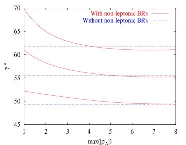
To further illustrate this point, we have included in our analysis the constraint coming from $BR(B\to K\pi,\pi\pi)$ using the model of ref. [25] and considered the dependence of the predicted value of $\gamma$ on the phenomenological parameter $\rho_{A}$. This free parameter is introduced in the model to account to some extent for the infrared divergences appearing in the perturbative calculation of power-suppressed corrections. According to ref. [25], the allowed range of variation of $\rho_{A}$ is $|\rho_{A}|<1$. We find instead that the data prefer larger values $|\rho_{A}|\sim 4$–$6$. Figure 4 shows that the value of $\gamma$, which we obtain by including constraints from non-leptonic $BR$s, deviates from the one of eq. (9) only for value of max$(|\rho_{A}|)\sim 1$–$3$. On the other hand, when $\rho_{A}$ is allowed to get the values preferred by the data, no new informations on $\gamma$ are obtained besides those coming from more reliable constraints. In other words, it is just the restricted range for $\rho_{A}$ adopted in ref.  [25] which originates the claimed “improvement” in the determination of the CKM parameters due to non-leptonic $BR$s. To our knowledge, this choice has no compelling theoretical or phenomenological basis.

We rather believe that, at present, our control of the hadronic uncertainties in the $B\to K\pi,\pi\pi$ $BR$s is not developed enough to allow using these modes for costraining the CKM parameters.

References

-
[1]
N. Cabibbo, Phys. Rev. Lett. 10 (1963) 531;
M. Kobayashi and T. Maskawa, Prog. Theor. Phys. 49 (1973) 652. - [2] L. Wolfenstein, Phys. Rev. Lett. 51 (1983) 1945.
- [3] A.J. Buras, M.E. Lautenbacher and G. Ostermaier, Phys. Rev. D50 (1994) 3433.
- [4] M. Ciuchini et al., JHEP 0107 (2001) 013 [arXiv:hep-ph/0012308].
- [5] T. Inami and C.S. Lim, Prog. Theor. Phys. 65 (1981) 297; ibid. 65 (1981) 1772.
- [6] A.J. Buras, M. Jamin and P.H. Weisz, Nucl. Phys. B347 (1990) 491.
[7]
F. Abe et al., CDF Collaboration, Phys. Rev. Lett.
74 (1995) 2626;
S. Abachi et al., D0 Collaboration, Phys. Rev. Lett. 74 (1995) 2632. -
[8]
S. Herrlich and U. Nierste, Nucl. Phys. B419 (1994) 192;
G. Buchalla, A.J.Buras and M.E. Lautenbacher, Rev. Mod. Phys. 68, (1996) 1125. - [9] Review of Particle Physics, Eur. Phys. J. C15 (2000) 1.
- [10] The LEP B Oscillation Working Group, http://lepbosc.web.cern.ch/LEPBOSC/.
- [11] V. Gimenez, L. Giusti, G. Martinelli and F. Rapuano, JHEP 0003 (2000) 018.
- [12] A. Hocker, H. Lacker, S. Laplace and F. Le Diberder, Eur. Phys. J. C 21 (2001) 225 [arXiv:hep-ph/0104062].
- [13] S. Stone, arXiv:hep-ph/0112008.
- [14] M. Lusignoli, L. Maiani, G. Martinelli and L. Reina, Nucl. Phys. B369 (1992) 139.
- [15] M. Ciuchini, E. Franco, G. Martinelli, L. Reina and L. Silvestrini, Z. Phys. C68 (1995) 239.
- [16] P. Paganini, F. Parodi, P. Roudeau and A. Stocchi, Phys. Scripta V. 58 (1998) 556.
- [17] F. Parodi, P. Roudeau and A. Stocchi, Nuovo Cim. 112A (1999) 833.
- [18] M. Ciuchini, E. Franco, L. Giusti, V. Lubicz and G. Martinelli, Nucl. Phys. B573 (2000) 201.
- [19] see e.g. N. Katayama (Belle collab.), these Proceedings.
- [20] P. Checchia, E. Piotto, F. Simonetto, Eur. Phys. Lett. 47 (1999) 113011.
- [21] R. Barbieri, L. Hall, A. Stocchi and N. Weiner, Phys. Lett. B425 (1998) 119;
- [22] D. Jaffe, S. Youssef, Comput.Phys.Commun. 101 (1997) 206
- [23] D. Becirevic et al., Nucl. Phys. B 618 (2001) 241 [arXiv:hep-lat/0002025].
- [24] F. Caravaglios, F. Parodi, P. Roudeau, A. Stocchi, hep-ph/0002171, Proceedings of “BCP 99”, Taipei, Taiwan, Dec. 3-7 1999.
- [25] M. Beneke, G. Buchalla, M. Neubert and C. T. Sachrajda, Nucl. Phys. B 606 (2001) 245 [arXiv:hep-ph/0104110].