Solar and atmospheric neutrinos: a solution with large extra dimensions

Abstract

We have studied [1] flavor neutrinos confined to our four-dimensional world coupled to one ”bulk” state, i.e., a Kaluza-Klein tower. Within a minimal model, we accomodate existing experimental constraints (CHOOZ experiment, solar and atmospheric data). No direct flavor oscillations nor MWS effects are needed. An energy independent suppression is produced at large distances.

1 Introduction

The possibility of ”large extra dimensions”, i.e., with (at least) one compactification radius close to the current validity limit of Newton’s law of gravitation ($\sim$ 0.1 mm), raises considerable interest. It could also solve the hierarchy problem by providing us with a new fundamental scale at an energy possibly as small as 1 TeV [2].

Neutrino physics is a favored area to study this possibility. A right-handed, sterile neutrino does not experience any of the gauge interactions and is therefore not confined to our four-dimensional brane; it is thus, other than the graviton, an ideal tool to probe the ”bulk” of space. The bulk states appear to us (due to compactification of the extra dimensions) as so-called Kaluza-Klein towers of states [3]. Recent works [4, 5, 6, 7] have shown that it is, at least partially, possible to accommodate experimental constraints on neutrinos within this setup.

We explore further possibilities, focusing on the unique properties of the model. Quite specifically, neutrinos in this scheme can ”escape” for part of the time to extra dimensions, resulting in a reduced average probability of detection in our world. While similar in a way to a fast unresolved oscillation between flavor and sterile neutrinos, this differs both by the time development of the effect and by the possible depth of the suppression.

2 Two neutrinos coupled to one bulk fermion: the 2-1 model

The simplest model is constituted by one left-handed neutrino state $\nu_{1}$ which lives in our 3+1 dimensional world coupled with one singlet ”bulk” massless fermion field. Since the latter lives in all dimensions, from our world’s point of view, it appears, after compactification, as a Kaluza-Klein (KK) tower, i.e., an infinite number of four-dimensional spinors.

The analysis presented here is based on a reduction of the theory from 4+1 to 3+1 dimensions. However, to guarantee a low scale for the unification of gravity with all forces, more extra dimensions are needed. We will assume that their compactification radii are small enough that they don’t affect the analysis. The pattern is now well established (see e.g. [4, 6]) and we will only recall the basic equations and results. The action used is the following :

$$S=\int d^{4}x\,dy\;\overline{\Psi}i\Gamma_{A}\partial^{A}\Psi+\int d^{4}x\{\overline{\nu}_{1}i\gamma_{\mu}\partial^{\mu}\nu_{1}+\lambda\overline{\nu}_{1}\Psi(x^{\mu},y=0)H(x^{\mu})+h.c.\}$$ (1)

where $A=0,...,4$ and $x^{4}=y$ is the extra dimension. The Yukawa coupling between the usual Higgs scalar, the weak eigenstate neutrino $\nu_{1}$ and the bulk fermion operates at $y=0$, which is the 3+1 dimensional brane of our world.

The fifth dimension is taken to be a circle of radius $R$. As usual, the bulk fermion $\Psi$ is expanded in eigenmodes. One then integrates over the fifth dimension. Eventually, one has to diagonalize the mass matrix (eigenvalues noted $\lambda_{n}$) and write the neutrino in terms of the mass eigenstates :

$$\lambda_{n}=\pi\xi^{2}\cot(\pi\;\lambda_{n})\;\;{\rm;}\;\left|\nu_{1}\right\rangle=\sum_{n=0}^{\infty}U_{0n}\left|\nu_{\lambda_{n}}\right\rangle\;\;{\rm;}\;U_{0n}^{2}=\frac{2}{1+\pi^{2}\xi^{2}+\frac{\lambda_{n}^{2}}{\xi^{2}}}$$ (2)

where $\xi\equiv\frac{m}{1/R}$ measures the strength of the Yukawa coupling .

The survival amplitude $A_{\nu_{1}\nu_{1}}$and probability $P_{\nu_{1}\nu_{1}}$ are given by

$$A_{\nu_{1}\nu_{1}} = \sum_{n=0}^{\infty}U_{0n}^{2}e^{\,i\,\lambda_{n}^{2}x}$$ (3)

$$P_{\nu_{1}\nu_{1}} = \sum_{n=0}^{\infty}U_{0n}^{4}+\sum\sum_{n\neq m}U_{0n}^{2}U_{0m}^{2}\cos\left[\left(\lambda_{n}^{2}-\lambda_{m}^{2}\right)x\right]$$ (4)

$${\rm where}\;\;\;x = \frac{L}{2ER^{2}}\approx 10^{-7}\frac{\left(L/{\rm km}\right)}{(E/{\rm GeV})(R/{\rm mm})^{2}}$$

We have shown in Ref.[1] that for $\nu_{1}=\nu_{e}$, it is possible to accomadate the CHOOZ contraint with a global $L/E$ independent solar suppression (free of MSW effect) but an atmospheric $\nu_{e}$ suppression is then expected. To reconcile with the data in that case, one needs the MSW effect [4, 6, 7]. To keep the solar suppression $L/E$ independent, we do not further investigate this possibility. $\nu_{1}$ can however be a linear combination of flavor states. Indeed if we describe the coupling of two flavor neutrinos to the bulk neutrino by the Lagrangian

$${\cal L}=\lambda_{e}\overline{\nu}_{e}\Psi(x^{\mu},y=0)H(x^{\mu})+\lambda_{\mu}\overline{\nu}_{\mu}\Psi(x^{\mu},y=0)H(x^{\mu}){\rm,}$$ (5)

we recover the previous action (1) by a rotation of the flavor base

$$\nu_{1} = \cos\theta\;\nu_{e}+\sin\theta\;\nu_{\mu}$$ (6)

$$\nu_{2} = -\sin\theta\;\nu_{e}+\cos\theta\;\nu_{\mu}{\rm,}$$ (7)

with $\cos\theta=\frac{m_{e}}{m}$ , $\sin\theta=\frac{m_{\mu}}{m}$, $m=\sqrt{m_{e}^{2}+m_{\mu}^{2}}$ and $m_{e,\mu}=\frac{\lambda_{e,\mu}v}{\sqrt{2\pi R}}$ . The mixing with bulk states remains unchanged for $\nu_{1}$. The orthogonal combination $\nu_{2}$ remains massless and decouples from the bulk neutrino. A new phenomenological parameter, the mixing angle $\theta$ now plays a crucial role in the survival probabilities of the flavor neutrinos,

$$P_{\nu_{e}\nu_{e}} = \cos^{4}\theta\;P_{\nu_{1}\nu_{1}}+\sin^{4}\theta+2\sin^{2}\theta\;\cos^{2}\theta\;\textrm{Re}\left(A_{\nu_{1}\nu_{1}}\right)$$ (8)

$$P_{\nu_{\mu}\nu_{\mu}} = \sin^{4}\theta\;P_{\nu_{1}\nu_{1}}+\cos^{4}\theta+2\sin^{2}\theta\;\cos^{2}\theta\;\textrm{Re}\left(A_{\nu_{1}\nu_{1}}\right)$$ (9)

and a flavor transition is possible through the bulk states

$$P_{\nu_{e}\nu_{\mu}}=P_{\nu_{\mu}\nu_{e}}=\sin^{2}\theta\ \cos^{2}\theta\ (P_{\nu_{1}\nu_{1}}-2\textrm{Re}\left(A_{\nu_{1}\nu_{1}}\right)+1)$$ (10)

This model (hereafter called the 2-1 model) has 3 degrees of freedom, $(\xi,\theta,R)$, to fit the experimental data. We should also stress that $\theta$ is not the $\nu_{e}-\nu_{\mu}$ mixing angle . Such mixing arises, but only as a result of the independent coupling of both states to the bulk neutrino.

2.1 Confrontation of the model with experimental data

We discuss here how the experimental constraints can be accounted for in our 2-1 model. A discussion of the experimental data themselves and related references can be found in Ref.[1].

The solar neutrino deficit is accounted for if the $\nu_{e}$ mean survival probability $\left<P_{\nu_{e}\nu_{e}}\right>$ at large $x$ ranges between 40% to 60% (as a result of the experimental errors and solar model uncertainties). This constraint defines a region in the plane $\xi-\theta$ (Fig. 6 in Ref.[1]). In models with large extra dimensions and if no MSW effects are playing, $\left<P_{\nu_{e}\nu_{e}}\right>$ is naturally constant at large $x$. Such a solution is the simplest interpretation of the absence of $L/E$ dependence in the SuperKamiokande solar neutrinos data. To prevent any $L/E$ dependence, we should also avoid MSW effects in the Sun or Earth.

As the Sun-Earth system is a very long-baseline one and as the solar core is large (typically, $x\sim 10^{5}$ and $\Delta x\sim 10^{2}\gg 1$ for solar neutrinos with $E\sim 1$ MeV and $R\sim 1$ mm), $\left<P_{\nu_{e}\nu_{e}}\right>$ is the only observable effect: the fast fluctuations of the survival probability are completely washed away, whatever the detector resolution.

The CHOOZ nuclear reactor experiment observes no $\overline{\nu}_{e}$ disappearance at a distance $L=1~{}$ km and a typical energy of 2 MeV. For given $\xi$ and $\theta$, a maximum admissible value of $x$, or equivalently, a minimum value of $R$ (the radius of the compactified extra dimension) results. A small coupling constant $\xi$ and a large mixing angle $\theta$ are preferred.

On the other hand, $1/R$ controls the typical mass difference between two consecutive Kaluza-Klein levels. Therefore, MSW resonant conversion will take place if $1/R$ is of the same magnitude order as the MSW potential. To avoid the MSW effect and consequently $L/E$ dependences in the mean survival probability, we can put an upper bound on $R$. Typically, $R_{\max}\simeq 10^{-2}$ mm. As a result, for some $\xi$ and $\theta$, this bound can be incompatible with the CHOOZ constraint (see Fig. 6 in Ref.[1]).

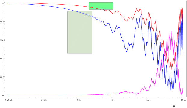
The $\overline{\nu}_{\mu}$ disappearance experiment K2K reveals some 30% deficit for 2 GeV neutrinos at a distance $L\simeq 250$ km. Since we have $x_{\rm K2K}\simeq 1/4\,x_{\rm CHOOZ}$, $\nu_{\mu}$’s are expected to disappear more than $\nu_{e}$’s. This requires $\theta>\pi/4$, and higher values of $\xi$ are favored, as $P_{\nu_{e}\nu_{e}}-P_{\nu_{\mu}\nu_{\mu}}\propto(1-P_{\nu_{1}\nu_{1}})$. However, even for the maximal allowed $\xi$, the preliminary result of K2K can only be accommodated by taking the large statistical error into account. The Fig. 1 shows a possible fit for $\nu_{e}$ and $\nu_{\mu}$, which solves the solar neutrino problem, and simultaneously satisfies the CHOOZ and K2K constraints.

Figure 1: Comparison of the 2-1 model with the CHOOZ and K2K constraints (highest curve is for $\nu_{e}$. $\xi=0.3$ and $\theta=1.05$, so that $\left<P_{\nu_{e}\nu_{e}}\right>\simeq 60\%$. The transition probability $P_{\nu_{e}\nu_{\mu}}$ is also depicted (lowest curve). The error bar (at 2$\sigma$ for CHOOZ; 1$\sigma$ for K2K) combines quadratically the statistical and systematic errors.

Figure 2: Expected atmospheric neutrino fluxes in the 2-1 model and the SuperKamiokande data. Same $\xi$ and $\theta$ have been used. The series of filled boxes show the $L/E$ dependence for the atmospheric $\nu_{e}$ and $\nu_{\mu}$, as observed by SuperKamiokande (1$\sigma$). The initial flux is normalized to 1 at $x=0$ and the data has been normalized by an overall 0.95 factor with respect to the raw data (instead of the usual $\sim$0.9 used by SuperKamiokande). The agreement with experimental data is quite remarkable. The boxes of both figures are taken as in ¹.

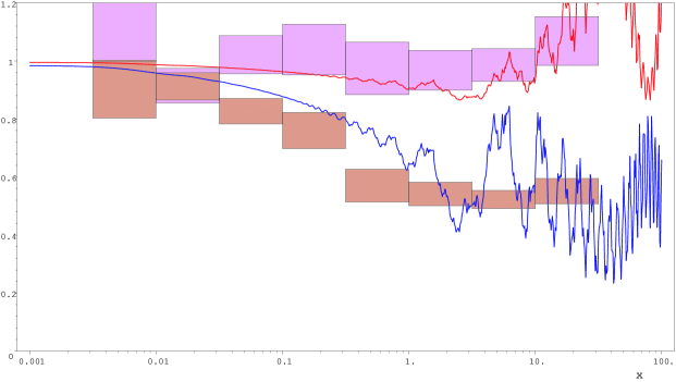
To discuss the atmospheric neutrinos, we recall that in the 2-1 model, a transition $\nu_{e}\rightarrow\nu_{\mu}$ or $\nu_{\mu}\rightarrow\nu_{e}$ becomes possible. The transition probability, as shown in Fig. 1, is non-negligible in the range of the atmospheric neutrinos. As the latter originate from the decay of the charged pions and kaons into muons and the subsequent decay of muons, the ratio of the neutrino initial fluxes $\phi^{(i)}_{\nu_{\mu}}/\phi^{(i)}_{\nu_{e}}$ is expected to be very close to 2, especially at low energy. Therefore, the expected neutrino flux in the 2-1 model is given by $\phi_{\nu_{e}}/\phi^{(i)}_{\nu_{e}}=P_{\nu_{e}\nu_{e}}+2\,P_{\nu_{\mu}\nu_{e}}$ and $\phi_{\nu_{\mu}}/\phi^{(i)}_{\nu_{\mu}}=P_{\nu_{\mu}\nu_{\mu}}+1/2\,P_{\nu_{e}\nu_{\mu}}$ (we don’t distinguish between $\nu$ and $\overline{\nu}$). As a result, the observed $\nu_{e}$ flux can be enhanced compared to the initial production flux. In Fig. 2, we see that this picture is in very good agreement with the SuperKamiokande results. Moreover models with extra dimensions escape at least partially the SuperKamiokande constraints on sterile neutrinos. Indeed, while oscillations are blocked by an MSW effect in the Earth in a $\nu_{\mu}$-$\nu_{s}$ maximal mixing picture, anti-neutrinos always find a resonant KK state to oscillate to in the $\nu_{\mu}$-$\nu_{KK}$ model[1].

We are left with the constraints of KARMEN and LSND. The negative result of the KARMEN experiment can easily be accommodated but our model can never comply with the LSND results, for any allowed values of $\theta$ and $\xi$. This however can be understood: the 2-1 model provides two mass scales, $\lambda_{0}/R\approx\xi/R=m$ and $\lambda_{1}/R\approx 1/R$, allowing to account for the solar and atmospheric anomalies. The contributions of the KK tower can in principle account for the LSND results, but it turns out that the effect is too weak.

We also point out that the astrophysical bound could be partly evaded in this model, since the disappearance of $\nu_{e}$ or $\nu_{\mu}$ in the extra dimensions is never complete (see [8]; for discussions on astrophysical and cosmological constraints, see, e.g., [6, 9]).

3 Conclusions

We have shown that a simple model with 2 massless flavor neutrinos, namely $\nu_{e}$ and $\nu_{\mu}$, coupled to one Kaluza-Klein tower meets most experimental constraints (except for LSND), and differs from the oscillation image by the energy-dependence of the neutrino disappearance. This model can be developed by adding extra parameters in the form of bare masses for the neutrinos, while simply increasing the number of neutrinos coupled to the Kaluza-Klein states brings little gain.

References

- [1] N. Cosme, J. M. Frère, Y. Gouverneur, F. S. Ling, D. Monderen and V. Van Elewyck, accepted for publication in Phys. Rev. D, hep-ph/0010192.
- [2] N. Arkani-Hamed, S. Dimopoulos and G. Dvali, Phys. Lett. B 429 (1998) 263; I. Antoniadis, N. Arkani-Hamed, S. Dimopoulos and G. Dvali, Phys. Lett. B 436 (1998) 257.
- [3] N. Arkani-Hamed, S. Dimopoulos, G. Dvali and J. March-Russell, hep-ph/9811448; K. R. Dienes, E. Dudas, T. Gherghetta, Nucl. Phys. B 557 (1999) 25; R. N. Mohapatra, S. Nandi and A. Pérez-Lorenzana, Phys. Lett. B 466 (1999) 115; A. Das and O. C. Kong, Phys. Lett. B 470 (1999) 149; A. Lukas, P. Ramond, A. Romanino and G. G. Ross, hep-ph/0011295.
- [4] G. Dvali and A. Y. Smirnov, Nucl. Phys. B 563 (1999) 63.
- [5] A. Pérez-Lorenzana, hep-ph/0008333.
- [6] R. Barbieri, P. Creminelli and A. Strumia, Nucl. Phys. B 585 (2000) 28.
- [7] R. N. Mohapatra and A. Pérez-Lorenzana, Nucl. Phys. B 593 (2001) 451; D. O. Caldwell, R. N. Mohapatra and S. J. Yellin, hep-ph/0010353. A. Lukas, P. Ramond, A. Romanino and G. G. Ross, Phys. Lett. B 495 (2000) 136; A. Ioannisian and J. W. Valle, hep-ph/9911349; E. Ma, G. Rajasekaran and U. Sarkar, Phys. Lett. B 495 (2000) 363.
- [8] K. R. Dienes and I. Sarcevic, Phys. Lett. B 500 (2001) 133.
- [9] G. C. McLaughlin and J. N. Ng, Phys. Lett. B 470 (1999) 157; K. Agashe and G. Wu, Phys. Lett. B 498 (2001) 230; K. Abazajian, G. M. Fuller and M. Patel, hep-ph/0011048. K. Abazajian, G. M. Fuller and M. Patel, astro-ph/0101524.