SAGA-HE-170-01, TMU-NT-01-01
 
 
Determination of nuclear parton distributions

Abstract

Parametrization of nuclear parton distributions is investigated in the leading order of $\alpha_{s}$. The parton distributions are provided at $Q^{2}$=1 GeV² with a number of parameters, which are determined by a $\chi^{2}$ analysis of the data on nuclear structure functions. Quadratic or cubic functional form is assumed for the initial distributions. Although valence quark distributions in the medium $x$ region are relatively well determined, the small $x$ distributions depend slightly on the assumed functional form. It is difficult to determine the antiquark distributions at medium $x$ and gluon distributions. From the analysis, we propose parton distributions at $Q^{2}$=1 GeV² for nuclei from deuteron to heavy ones with the mass number $A\sim 208$. They are provided either analytical expressions or computer subroutines for practical usage. Our studies should be important for understanding the physics mechanism of the nuclear modification and also for applications to heavy-ion reactions. This kind of nuclear parametrization should also affect existing parametrization studies in the nucleon because “nuclear” data are partially used for obtaining the optimum distributions in the “nucleon”.

I Introduction

Unpolarized parton distributions in the nucleon are now well determined in the region from very small $x$ to large $x$ by using various experimental data. There are abundant data on electron and muon deep inelastic scattering. In addition, there are available data from neutrino reactions, Drell-Yan processes, $W$ productions, direct photon productions, and others. The optimum parton distributions are determined so as to fit these experimental data. Initial distributions are assumed at a fixed $Q^{2}$ with parameters, which are determined by a $\chi^{2}$ analysis. Now, there are three major groups, CTEQ (Coordinated Theoretical/Experimental Project on QCD Phenomenology and Tests of the Standard Model) cteq5 , GRV (Glück, Reya, and Vogt) grv98 , and MRS (Martin, Roberts, and Stirling) mrs99 , which have been investigating the unpolarized parametrization.

Because the distributions themselves are associated with nonperturbative Quantum Chromodynamics (QCD), they cannot be described precisely by theoretical methods at this stage. Therefore, the determination enables us to understand internal structure of the nucleon, hence to test the nonperturbative hadron models. In addition, the parton distributions are always necessary for calculating cross sections of high-energy reactions involving a nucleon. Furthermore, there is other importance in determining future physics direction. If the distributions are precisely known, any experimental deviation from theoretical predictions should indicate new physics beyond the standard model, for example a signature of subquark system.

The situation is worse in polarized distributions. Longitudinally polarized distributions have been investigated in the last decade. From the analyses of many polarized electron and muon deep inelastic experimental data, several parametrizations have been proposed. Neutrino, Drell-Yan, and other data are not available unlike the unpolarized studies, so that antiquark and gluon distributions cannot be determined accurately at this stage aac . More precise determination should be done by the polarized Relativistic Heavy Ion Collider (RHIC) experiments in the near future.

It is well known that nuclear parton distributions are modified from the corresponding ones in the nucleon according to the measurements of nuclear $F_{2}$ structure functions f2sum . Because $F_{2}$ is expected to be dominated by sea- and valence-quark distributions at small and large $x$, respectively, the modification of each distribution should be determined by the $F_{2}$ measurements in the small or large $x$ region. However, it is not straightforward to find the detailed $x$ dependence of these distributions. Furthermore, it is also not obvious how nuclear gluon distributions are constrained by the $F_{2}$ data. There are trials to obtain the distributions from the data in a model dependent way saga and in a model independent way by Eskola, Kolhinen, and Ruuskanen helsinki ; however, they are not $\chi^{2}$ analyses. Therefore, this paper is intended to pioneer the $\chi^{2}$ analysis study for obtaining optimum nuclear parton distributions mumbai .

There are following motivations for investigating the nuclear parametrization. The first purpose is to test various nuclear models for describing the nuclear structure functions. From the detailed comparison, the most appropriate nuclear model could be determined in the high-energy region. Furthermore, we may be able to find an explicit subnucleon signature in nuclear physics. The second purpose is to calculate cross sections of high-energy nuclear reactions accurately. For example, precise initial conditions must be known in heavy-ion reactions for finding a signature of quark-gluon plasma. In many calculations, nuclear parton distributions are simply assumed to be the same as the corresponding ones in the nucleon. The third purpose is related to the aforementioned nucleon parametrization. In obtaining parton distributions in the “nucleon”, some “nuclear” data are actually used without considering the nuclear modification. For example, neutrino $F_{3}$ data are essential for determining the valence-quark distributions in the nucleon. However, most data are taken for the iron target! In future, accurate neutrino-proton scattering data could be taken if a neutrino factory is realized sknu . It is inevitable to utilize the nuclear data at this stage. Therefore, our nuclear studies should be useful for improving the present parametrizations in the nucleon.

This paper consists of the following. First, dependence of the mass number $A$ and scaling variable $x$ is discussed in II. Then, our analysis method is explained in III, and results are presented in IV. Obtained distributions are provided in Sec. V for practical usage. Finally, our nuclear parametrization studies are summarized in section VI.

II Functional form of nuclear parton distributions

Because there is no prior $\chi^{2}$ analysis on the nuclear parametrization, we should inevitably take the $A$ and $x$ dependence as simple as possible for the first step trial. However, the functional form of $x$ should be taken independently from any theoretical nuclear models as a fair analysis. Our standpoint is to test the models without relying on them. We discuss an appropriate functional form of the distributions in the following subsections.

II.1 $A$ dependence

There is some consensus on physics mechanism of nuclear modification in each $x$ region. Because different mechanisms contribute to the modification depending on the $x$ region, the $A$ dependence could vary in different $x$ regions. However, in order to simplify the analysis, we introduce a rather bold assumption: The $A$ dependence is assumed to be proportional to $1/A^{1/3}$. Physics behind this idea is discussed by Day and Sick in Ref. ds . In any nuclear reaction, the cross section is expressed in terms of nuclear volume and surface contributions:

$$\sigma_{A}=A\,\sigma_{V}+A^{2/3}\sigma_{S}.$$ (1)

Therefore, the cross section per nucleon is given as

$$\frac{\sigma_{A}}{A}=\sigma_{V}+\frac{1}{A^{1/3}}\sigma_{S}.$$ (2)

If $\sigma_{V}$ and $\sigma_{S}$ depend weakly on $A$, the $1/A^{1/3}$ dependence makes sense as the leading approximation. In fact, according to the measured $F_{2}^{A}/F_{2}^{D}$ data, this $A$ dependence is justified ds .

Figure 1: $A$ dependence of measured $F_{2}^{A}/F_{2}^{D}$ ratios at $x=0.5$.

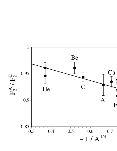
In order to illustrate the justification, we show actual $F_{2}^{A}/F_{2}^{D}$ data as a function of $1-1/A^{1/3}$ at $x=0.5$ together with a straight line in Fig. 1. It is obvious from the figure that measured ratios are well reproduced by the line with the $1-1/A^{1/3}$ dependence. We also looked at other regions, for example, the small $x$ region and found that the data could be described by this $A$ dependence. In this way, we decided to employ this simple assumption. Of course, the $1/A^{1/3}$ dependence may be an oversimplification. Detailed studies of the $A$ dependence are left as a future research topic.

We should mention, however, that the exact $1-1/A^{1/3}$ dependence is not completely consistent with the conditions of nuclear charge, baryon number, and momentum. We need to assign fine-tuning parameters which adjust the nuclear dependence. The details will be explained in the next subsection below Eq. (8).

II.2 $x$ dependence

Available nuclear data on the structure function $F_{2}^{A}$ are taken in fixed-target experiments at this stage, and they are shown as a function of $Q^{2}$ and $x\equiv Q^{2}/(2m\nu)$, where $\nu$ is the energy transfer, $m$ is the nucleon mass, and $Q^{2}$ is given by $Q^{2}\equiv-q^{2}$ with the virtual photon momentum $q$. The initial nuclear parton distributions are provided at a fixed $Q^{2}$ ($\equiv Q_{0}^{2}$), and they are taken as

$$f_{i}^{A}(x,Q_{0}^{2})=w_{i}(x,A,Z)\,f_{i}(x,Q_{0}^{2}),$$ (3)

where $f_{i}^{A}(x,Q_{0}^{2})$ is the parton distribution with type $i$ in the nucleus $A$ and $f_{i}(x,Q_{0}^{2})$ is the corresponding parton distribution in the nucleon. We call $w_{i}(x,A,Z)$ a weight function, which takes into account the nuclear modification.

We lose a piece of information by using Eq. (3). A scaling variable for the lepton-nucleus scattering could be given by $x_{A}\equiv Q^{2}/(2p_{A}\cdot q)$, where $p_{A}$ is the momentum of the target nucleus. We could define another variable for lepton-nucleon scattering as $x_{N}\equiv Q^{2}/(2p\cdot q)$ with the nucleon momentum $p$ within the nucleus. The variable $x_{A}$ indicates the momentum fraction of a struck-quark in the nucleus and it is kinematically restricted as $0<x_{A}<1$. Because of these definitions, we have the relation $x=x_{A}M_{A}/m$, where $M_{A}$ is the nuclear mass, in a fixed target reaction. In this way, we find that the range of nuclear parton distributions is given by $0<x<A$. Therefore, the extremely large $x$ region ($x>1$) cannot be described in our present approach with Eq. (3) because the distributions in the nucleon vanish: $f_{i}(x>1,Q_{0}^{2})=0$.

There are following reasons for using Eq. (3) irrespective of this issue. First, there are not so many experimental data in this $x$ region. Second, even if finite parton distributions are assumed at the initial point $Q_{0}^{2}$, there is no reliable theoretical tool to evolve them to larger $Q^{2}$ points where the data exist. Therefore, such large $x$ distributions cannot be accommodated in our $\chi^{2}$ analysis. There is a nuclear $Q^{2}$ evolution code in Ref. bf1 ; however, the original evolution equations are written in the range $0<x<1$ mq . Third, because the nuclear modification is generally in the 10$-$30% range for medium and large size nuclei, it is much easier to investigate the modification from the distributions in the nucleon rather than the absolute nuclear distributions themselves. Forth, the structure functions $F_{2}^{A}$ or parton distributions are tiny at $x>1$, so that they do not affect the calculated cross sections significantly unless an extreme kinematical condition is chosen.

Now, we proceed to the actual $x$ dependence.

(1) Nuclear modification $\bf\propto$ $\bf 1-1/A^{1/3}$

As concluded in the previous subsection, the nuclear modification part of $w_{i}(x,A,Z)$ is assumed to be proportional to $1-1/A^{1/3}$:

$$w_{i}(x,A,Z)=1+\left(1-\frac{1}{A^{1/3}}\right)(\text{function of $x$, $A$, and $Z$}).$$ (4)

(2) Introduction of $\bf 1/(1-x)^{\beta}$ factor

The nuclear parton distributions have finite values even at $x=1$ in principle, so that the weight function should behave as

$$w_{i}(x\rightarrow 1,A,Z)=\frac{f_{i}^{A}(x\rightarrow 1)}{f_{i}(x\rightarrow 1)}\rightarrow\infty.$$ (5)

This equation should hold whatever the modification mechanism is. In order to reproduce this feature, the factor $1/(1-x)^{\beta_{i}}$ is introduced in the $x$ dependent function part of Eq. (4) with a parameter $\beta_{i}(>0)$:

$$(\text{function of $x$, $A$, and $Z$})\propto\frac{1}{(1-x)^{\beta_{i}}}.$$ (6)

(3) Saturation of shadowing or antishadowing

We assume saturation of the function $w_{i}(x,A,Z)$ at $x\rightarrow 0$. It is considered to be a reasonable assumption unless there is a peculiar mechanism to produce singular behavior at small $x$. As far as the experimental $F_{2}^{A}/F_{2}^{D}$ data suggest, the shadowing at small $x$ tends to saturate as $x\rightarrow 0$. If this saturation is assumed, the weight function $w_{i}$ becomes

$$w_{i}(x\rightarrow 0,A,Z)=1+\left(1-\frac{1}{A^{1/3}}\right)a_{i}(A,Z),$$ (7)

where $a_{i}$ is the parameter which controls shadowing or antishadowing magnitude.

From these discussions, an appropriate functional form becomes

$$w_{i}(x,A,Z)=1+\left(1-\frac{1}{A^{1/3}}\right)\frac{a_{i}(A,Z)+H_{i}(x)}{(1-x)^{\beta_{i}}},$$ (8)

where the additional $x$ dependent part is written as $H_{i}(x)$, and it determines minute $x$ dependent shape. The reason why we let the parameters $a_{i}$ depend on $A$ and $Z$ is the following. As explained in the next section, there are three obvious constraints, charge, baryon number, and total momentum, on the nuclear distributions. If these conditions are satisfied for a nucleus, they are also fulfilled for other nuclei with the same $Z/A$ ratio. For example, the conditions could be satisfied for all the isoscalar nuclei. However, we also analyze nuclei with different $Z/A$ ratios. Then, even if the three conditions are satisfied in a certain nucleus, they are not strictly fulfilled for other nuclei with different $Z/A$ factors. In order to avoid this kind of failure, nuclear dependence is assumed for the parameters $a_{i}$ in the valence-quark and gluon functions. They are determined by the $\chi^{2}$ analysis so as to satisfy the three conditions for any nucleus.

Because this is the first $\chi^{2}$ trial, we would like to simplify the functional form of $H_{i}(x)$ as much as possible. A simple idea is to expand it in a polynomial form $H_{i}(x)=b_{i}x+c_{i}x^{2}+\cdot\cdot\cdot$. An advantage of this functional form is that the polynomials of $x$ and $1-x$ are very easy to be handled in the Mellin-transformation method of the $Q^{2}$ evolution. Because a direct $x$-space solution bf1 is used in our $Q^{2}$ evolution, it does not matter in our present analysis. However, it is important for public usage if we consider the fact that many researchers use the Mellin transformation as their $Q^{2}$ evolution method.

It is obvious that $H_{i}(x)=b_{i}x$ cannot explain the complicated $F_{2}^{A}/F_{2}^{D}$ shape in the medium $x$ region. Therefore, the simplest yet realistic choice is to take $H_{i}(x)=b_{i}x+c_{i}x^{2}$. This seems to be acceptable in the sense that the medium $x$ depletion of $F_{2}^{A}/F_{2}^{D}$ can be explained together with the $F_{2}^{A}$ shadowing at small $x$. However, if the depletion is described by the valence-quark behavior as our common sense suggests, the valence-quark distributions show anti-shadowing at small $x$ due to the baryon-number conservation. As explained in Refs.F3A ; sknu , it is not obvious at this stage whether the valence distributions indicate shadowing or antishadowing without accurate neutrino-deuteron scattering data and also small $x$ nuclear data. Therefore, this functional form should be considered as one of possible options:

$$w_{i}(x,A,Z) =1+\left(1-\frac{1}{A^{1/3}}\right)\frac{a_{i}(A,Z)+b_{i}x+c_{i}x^{2}}{(1-x)^{\beta_{i}}}$$

$$\text{``quadratic type"}.$$ (9)

We call this weight function the quadratic type in the following discussions.

If the next polynomial term $d_{i}x^{3}$ is added in addition, the function becomes more flexible in fitting the data:

$$w_{i}(x,A,Z) =1+\left(1-\frac{1}{A^{1/3}}\right)\frac{a_{i}(A,Z)+b_{i}x+c_{i}x^{2}+d_{i}x^{3}}{(1-x)^{\beta_{i}}}$$

$$\text{``cubic type"}.$$ (10)

We call this weight function the cubic type. An advantage of the additional term is, for example, that the weight function becomes flexible enough to accommodate both possibilities, shadowing and anti-shadowing, in the valence-quark distributions. A disadvantage is that the number of total parameters becomes larger, so that the total computing time becomes longer.

These quadratic and cubic functional types are used in our $\chi^{2}$ analyses. Finding the optimum point for the parametrization set, we expect to explain the major features of the measured $F_{2}^{A}/F_{2}^{D}$ ratios.

III Analysis method

In addition to the initial functional form, there are other important factors for performing the $\chi^{2}$ analysis. In this section, the details are discussed on used experimental data and our $\chi^{2}$ analysis method.

III.1 Experimental data

There are many available experimental data which could indicate nuclear parton distributions. However, we restrict the data to those taken by the deep inelastic electron and muon scattering. Neutrino, Drell-Yan, and other hadron-collider data are not used in our present analysis with the following reasons. At first, we would like to investigate how the distributions are determined solely by the electron and muon scattering data. Next, as it is mentioned in Sec. I, nuclear modification of $F_{3}$ is not measured in the neutrino scattering. In hadron-hadron reactions, there are also issues of $K$-factors and final state interactions. In a future version of our analysis, we will consider to include other data.

Table 1: Nuclear species, references, and data numbers are listed for the used experimental data with $Q^{2}\geq 1$ GeV².

nucleus	experiment	reference	# of data
He	SLAC-E139	slac94	18
	NMC-95	nmc95	17
Li	NMC-95	nmc95	17
Be	SLAC-E139	slac94	17
C	EMC-88	emc88	9
	EMC-90	emc90	5
	SLAC-E139	slac94	7
	NMC-95	nmc95	17
	FNAL-E665-95	e665-95	5
N	BCDMS-85	bcdms85	9
Al	SLAC-E49	slac83B	18
	SLAC-E139	slac94	17
Ca	EMC-90	emc90	5
	NMC-95	nmc95	16
	SLAC-E139	slac94	7
	FNAL-E665-95	e665-95	5
Fe	SLAC-E87	slac83	14
	SLAC-E140	slac88	10
	SLAC-E139	slac94	23
	BCDMS-87	bcdms87	10
Cu	EMC-93	emc93	19
Ag	SLAC-E139	slac94	7
Sn	EMC-88	emc88	8
Xe	FNAL-E665-92	e665-92	5
Au	SLAC-E140	slac88	1
	SLAC-E139	slac94	18
Pb	FNAL-E665-95	e665-95	5
total			309

At this stage, the available nuclear data are mainly on the $F_{2}$ structure functions in the electron and muon scattering. Experimental results are shown by the ratio

$$R_{F_{2}}^{A}(x,Q^{2})\equiv\frac{F_{2}^{A}(x,Q^{2})}{F_{2}^{D}(x,Q^{2})}.$$ (1)

Information about the used experimental data is given in Table 1, where nuclear species, references, and data numbers are listed. The experimental data are taken from the publications by the European Muon Collaboration (EMC) emc88 ; emc90 ; emc93 at the European Organization for Nuclear Research (CERN), the E49, E87, E139, and E140 Collaborations slac83 ; slac83B ; slac88 ; slac94 at the Stanford Linear Accelerator Center (SLAC), the Bologna-CERN-Dubna-Munich-Saclay (BCDMS) Collaboration bcdms85 ; bcdms87 at CERN, the New Muon Collaboration (NMC) nmc95 at CERN, the E665 Collaboration e665-92 ; e665-95 at the Fermi National Accelerator Laboratory (FNAL). The used data are for the nuclei: helium (He), lithium (Li), beryllium (Be), carbon (C), nitrogen (N), aluminum (Al), calcium (Ca), iron (Fe), copper (Cu), silver (Ag), tin (Sn), xenon (Xe), gold (Au), and lead (Pb). As explained in the next subsection, $Q_{0}^{2}$=1 GeV² is taken as the point where the parton distributions are defined. Because the published data include smaller $Q^{2}$ points, it is necessary to choose the ones with large enough $Q^{2}$ which could be considered in the perturbative QCD region. The only data with $Q^{2}\geq 1$ GeV² are taken into account in the $\chi^{2}$ analysis. The total number of the data is 309.

Figure 2: Kinematical range is shown by plotting $x$ and $Q^{2}$ points of the used data.

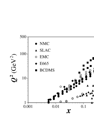
We show the $x$ and $Q^{2}$ points of the employed data in Fig. 2. The SLAC data are restricted to the large $x$ and small $Q^{2}$ region. Because the SLAC data are taken for many nuclear species, their data are very valuable for our analysis. However, they cannot address the issue of shadowing due to the lack of small $x$ measurements. The BCDMS data are also taken in the large $x$ region. The difference from the SLAC measurements is that the BCDMS data have large $Q^{2}$ values. There exist a large $Q^{2}$ gap between the SLAC and BCDMS data sets, which may enable us to investigate nuclear $Q^{2}$ evolution. On the other hand, the EMC, NMC, E665 data are almost in the same kinematical range. Because these data include small $x$ points, it is possible to investigate the shadowing region as well as the medium-$x$ modification part. However, the data have rather small $Q^{2}$ values in a restricted $Q^{2}$ range at small $x$. It suggests that it is difficult to determine the nuclear gluon distributions from the scaling violation at small $x$. In order to obtain the smaller $x$ or larger $Q^{2}$ data than those in Fig. 2, we should wait for a next generation project such as HERA-eA ahera or eRHIC erhic .

III.2 $\chi^{2}$ analysis

Our analysis is done in the leading order (LO) of $\alpha_{s}$. The structure function $F_{2}^{A}$ is expressed in a parton model as

$$F_{2}^{A}(x,Q^{2})=\sum_{q}e_{q}^{2}x[q^{A}(x,Q^{2})+\bar{q}^{A}(x,Q^{2})],$$ (2)

where $e_{q}$ is the quark charge, and $q^{A}$ ($\bar{q}^{A}$) is the quark (antiquark) distribution in the nucleus $A$. It is noteworthy to mention here that the structure functions and the parton distributions are defined by those per nucleon throughout this paper. Although it is now established that each antiquark distribution is different in the nucleon skpr , there is no data which could suggest flavor dependent antiquark distributions in a nucleus skantiq ; fnal-pro . Therefore, we should inevitably assume flavor symmetric antiquark distributions:

$$\bar{u}^{A}=\bar{d}^{A}=\bar{s}^{A}\equiv\bar{q}^{A}.$$ (3)

Furthermore, the flavor number is taken three. Then, the structure function becomes a summation of valence-quark and antiquark distributions:

$$F_{2}^{A}(x,Q^{2})=\frac{x}{9}[4u_{v}^{A}(x,Q^{2})+d_{v}^{A}(x,Q^{2})+12\bar{q}^{A}(x,Q^{2})].$$ (4)

The gluon distribution $g^{A}(x,Q^{2})$ is not explicitly contained in the LO structure function; however, it contributes to $F_{2}^{A}$ through $Q^{2}$ evolution which is described by coupled integro-differential equations with $g^{A}(x,Q^{2})$. In this way, we need four types of distributions, $u_{v}^{A}$, $d_{v}^{A}$, $\bar{q}^{A}$, and $g^{A}$, for calculating the structure function $F_{2}^{A}$.

Because the valence-quark distributions in a nucleus are much different from the ones in the proton, we should be careful in defining the weight function $w_{i}(x,A,Z)$. If there were no nuclear modification, in other words, if a nucleus were described simply by a collection of protons and neutrons, the parton distributions in the nucleus $A$ are given by

$$Af_{i}^{A}(x,Q^{2})_{\text{no-mod}} =Zf_{i}^{p}(x,Q^{2})+Nf_{i}^{n}(x,Q^{2}),$$

$$\text{where}\ f_{i}=u_{v},d_{v},\bar{q},\text{or}\ g.$$ (5)

The functions $f_{i}^{p}(x,Q^{2})$ and $f_{i}^{n}(x,Q^{2})$ are $i$-type distributions in the proton and neutron, respectively. Isospin symmetry is usually assumed for the parton distributions in the proton and the neutron:

$$u_{v}^{n} =d_{v}^{p}\equiv d_{v}, \ \ \ d_{v}^{n} =u_{v}^{p}\equiv u_{v},$$

$$\bar{q}^{n} =\bar{q}^{p}\equiv\bar{q}, \ \ \ g^{n} =g^{p}\equiv g.$$ (6)

Then, the nuclear parton distributions become

$$u_{v}^{A}(x,Q^{2})_{\text{no-mod}} =\frac{Zu_{v}(x,Q^{2})+Nd_{v}(x,Q^{2})}{A},$$

$$d_{v}^{A}(x,Q^{2})_{\text{no-mod}} =\frac{Zd_{v}(x,Q^{2})+Nu_{v}(x,Q^{2})}{A},$$

$$\bar{q}^{A}(x,Q^{2})_{\text{no-mod}} =\bar{q}(x,Q^{2}),$$

$$g^{A}(x,Q^{2})_{\text{no-mod}} =g(x,Q^{2}).$$ (7)

As suggested by the $F_{2}^{A}/F_{2}^{D}$ measurements, 10$-$30% modification is expected for medium and large size nuclei. The modification from the expressions in Eq. (7) should be expressed by the functions $w_{i}(x,A,Z)$ at $Q_{0}^{2}$ as discussed in Sec. II:

$$u_{v}^{A}(x,Q_{0}^{2}) =w_{u_{v}}(x,A,Z)\,\frac{Zu_{v}(x,Q_{0}^{2})+Nd_{v}(x,Q_{0}^{2})}{A},$$

$$d_{v}^{A}(x,Q_{0}^{2}) =w_{d_{v}}(x,A,Z)\,\frac{Zd_{v}(x,Q_{0}^{2})+Nu_{v}(x,Q_{0}^{2})}{A},$$

$$\bar{q}^{A}(x,Q_{0}^{2}) =w_{\bar{q}}(x,A,Z)\,\bar{q}(x,Q_{0}^{2}),$$

$$g^{A}(x,Q_{0}^{2}) =w_{g}(x,A,Z)\,g(x,Q_{0}^{2}).$$ (8)

We would like to take small $Q_{0}^{2}$ value in order to accommodate experimental data as many as possible. On the other hand, because the Dokshitzer-Gribov-Lipatov-Altarelli-Parisi (DGLAP) equations are used for the $Q^{2}$ evolution, $Q_{0}^{2}$ should be large enough so that perturbative QCD can be applied. As a point which could compromise these conflicting requirements, $Q_{0}^{2}=$1 GeV² is taken.

Next, a set of parton distributions in the nucleon is selected. There are available CTEQ, GRV, and MRS distributions. However, analytical expressions are not given in the CTEQ paper cteq5 , and the GRV expressions are provided at small $Q^{2}$ (0.26 GeV²) grv98 . Therefore, we decided to use a LO set of MRST (Martin, Roberts, Stirling, and Thorne) mrst , which is conveniently defined at $Q_{0}^{2}$=1 GeV². In this way, we use the central gluon version of MRST-LO distributions with the scale parameter $\Lambda_{LO}=0.1741$ GeV in our $\chi^{2}$ analysis. Consequently, obtained nuclear distributions in Sec. IV become the MRST distributions in the limit $A\rightarrow 1$.

Because each function $w_{i}(x,A,Z)$ still has four or five parameters, it is necessary to reduce the total number as many as possible in order to become an efficient analysis. First, there are following obvious constraints (a), (b), and (c) for the nuclear distributions.

(a) Charge

Nuclear charge has to be the atomic number $Z$. It can be expressed in a parton model by considering an infinite momentum frame for the nucleus. Let us consider elastic scattering of a real photon with its momentum $|\vec{q}|\rightarrow 0$ from a nucleus. Because each parton is moving very fast, we could use a parton picture for describing the process. Then, the nuclear charge is given as

$$Z =\int dx\,A\left[\frac{2}{3}(u^{A}-\bar{u}^{A})-\frac{1}{3}(d^{A}-\bar{d}^{A})-\frac{1}{3}(s^{A}-\bar{s}^{A})\right]$$

$$=\int dx\,\frac{A}{3}\left[2\,u_{v}^{A}-d_{v}^{A}\right].$$ (9)

The second equation is obtained because there is no net strangeness in an ordinary nucleus although $s^{A}(x,Q^{2})$ could be different from $\bar{s}^{A}(x,Q^{2})$. The valence distributions are defined by $u_{v}^{A}\equiv u^{A}-\bar{u}^{A}$ and $d_{v}^{A}\equiv d^{A}-\bar{d}^{A}$ as usual.

(b) Baryon number

Baryon number of a nucleus is $A$, and it is expressed in the parton model as

$$A =\int dx\,A\left[\frac{1}{3}(u^{A}-\bar{u}^{A})+\frac{1}{3}(d^{A}-\bar{d}^{A})+\frac{1}{3}(s^{A}-\bar{s}^{A})\right]$$

$$=\int dx\,\frac{A}{3}\left[u_{v}^{A}+d_{v}^{A}\right].$$ (10)

(c) Momentum

Nuclear momentum is the addition of each parton contribution:

$$A =\int dx\,A\,x\left[u^{A}+\bar{u}^{A}+d^{A}+\bar{d}^{A}+s^{A}+\bar{s}^{A}+g^{A}\right]$$

$$=\int dx\,A\,x\left[u_{v}^{A}+d_{v}^{A}+6\,\bar{q}^{A}+g^{A}\right].$$ (11)

If the weight functions are the quadratic functional type, the distributions are expressed by the parameters, $a_{u_{v}}$, $a_{d_{v}}$, $b_{v}$, $c_{v}$, $\beta_{v}$, $a_{\bar{q}}$, $b_{\bar{q}}$, $c_{\bar{q}}$, $\beta_{\bar{q}}$, $a_{g}$, $b_{g}$, $c_{g}$, and $\beta_{g}$. Here, the valence up- and down-quark parameters are assumed to be the same except for $a_{u_{v}}$ and $a_{d_{v}}$ because both weight functions are expected to be similar. However, at least one parameter should be different in order to satisfy the conditions (a) and (b) simultaneously since there are data for non-isoscalar nuclei with $Z\neq N$. Among the parameters, three of them can be fixed by the conditions, (a), (b), and (c). We use these three conditions for determining $a_{u_{v}}$, $a_{d_{v}}$, and $a_{g}$.

There are still irrelevant parameters which could be removed from the parametrization. First, $\beta_{\bar{q}}$ and $\beta_{g}$ describe the functional shape of the antiquark and gluon distributions at large $x$. However, they are irrelevant in the sense that both distributions are extremely small at large $x$, for example $x\sim 0.8$. They are not expected to contribute to $F_{2}^{A}$ significantly in this $x$ region. Furthermore, the antiquark and gluon distributions themselves are not determined at such large $x$ in the nucleon. In this way, we decided to fix the parameters at $\beta_{\bar{q}}=\beta_{g}=1$. We checked the sensitivity of our $\chi^{2}$ analysis results to this choice. Even if $\beta_{\bar{q}}=\beta_{g}=0.5$ or 2 is taken, we found that the obtained $\chi^{2}$ changed very little. This fact indicates that $\chi^{2}$ is almost independent of these parameters. There is another irrelevant parameter. The gluon parameters $b_{g}$ and $c_{g}$ determine the functional form at medium and large $x$. However, the gluon distribution does not contribute to $F_{2}^{A}$ directly, so that the detailed $x$ dependence cannot be determined in the analysis. Therefore, $b_{g}$ is fixed at $b_{g}=-2c_{g}$ with the following consideration. The $\chi^{2}$ analysis tends to favor negative $c_{g}$. As far as $b_{g}$ is taken to be larger than $-c_{g}$, the choice does not affect the $\chi^{2}$ to a considerable extent. However, if $b_{g}$ is taken smaller than $-c_{g}$, it could contradict with the condition $w_{i}(x\rightarrow 1,A,Z)\rightarrow+\infty$ depending on the value of $a_{g}$. In this way, there are seven free parameters

$$b_{v},\ \ c_{v},\ \ \beta_{v},\ \ a_{\bar{q}},\ \ b_{\bar{q}},\ \ c_{\bar{q}},\ \ c_{g},$$ (12)

in the quadratic fit. There are additional parameters in the cubic fit. However, as far as the gluon distribution is concerned, we use the same quadratic form even in the cubic type analysis. The structure function $F_{2}$ is rather insensitive to the gluon distribution, especially in the LO analysis. It does not make much sense to introduce an additional parameter for the gluon in the $\chi^{2}$ analysis without the data which could restrict the gluon distribution. In this way, the actual parameters are

$$b_{v},\ \ c_{v},\ \ d_{v},\ \ \beta_{v},\ \ a_{\bar{q}},\ \ b_{\bar{q}},\ \ c_{\bar{q}},\ \ d_{\bar{q}},\ \ c_{g},$$ (13)

in the cubic fit.

In the theoretical calculations, the nuclei are assumed as ⁴He, ⁷Li, ⁹Be, ¹²C, ¹⁴N, ²⁷Al, ⁴⁰Ca, ⁵⁶Fe, ⁶³Cu, ¹⁰⁷Ag, ¹¹⁸Sn, ¹³¹Xe, ¹⁹⁷Au, and ²⁰⁸Pb. The initial nuclear distributions are provided at $Q^{2}=1$ GeV² with the parameters in Eq. (12) or (13). They are evolved to the experimental $Q^{2}$ points by the DGLAP evolution equations. Then, obtained structure-function ratios $R_{F_{2}}^{A}$ are compared with the experimental values for calculating

$$\chi^{2}=\sum_{j}\frac{(R_{F_{2},j}^{A,data}-R_{F_{2},j}^{A,theo})^{2}}{(\sigma_{j}^{data})^{2}},$$ (14)

where the experimental error is given by systematic and statistical errors as $(\sigma_{j}^{data})^{2}=(\sigma_{j}^{sys})^{2}+(\sigma_{j}^{stat})^{2}$. Although the deuteron structure function is sometimes assumed the same as the one for the nucleon saga ; helsinki , the deuteron modification is also taken into account in our analysis simply by setting $A=2$. With these preparations together with the CERN subroutine Minuit minuit , the optimum parameter set is obtained by minimizing $\chi^{2}$.

IV Results

Our analysis results are explained in Sec. IV.1 in comparison with the used experimental data. Then, obtained optimum nuclear parton distributions are discussed in Sec. IV.2.

IV.1 Comparison with data

Analysis results are shown for both quadratic and cubic types. A minimal functional form is the quadratic type according to the discussion in Sec. II.2. It is minimal in the sense that the major features of the measured ratios $R^{A}_{F_{2}}$ could be described in the whole $x$ region including increase at large $x\sim 0.9$, depletion at medium at $x\sim 0.6$, antishadowing at $x\sim 0.15$, and shadowing at small $x<0.05$ with a minimum number of parameters. However, there are some restrictions on the distribution shape, most significantly on the valence-quark distributions. In the cubic type analysis, the shape becomes more flexible due to the additional parameters. Because of the new freedoms, obtained $\chi_{min}^{2}$ should be smaller for the cubic type, however, by sacrificing the computation time.

Figure 3: Fitting results are compared with the helium data. The dashed and solid curves are for the quadratic and cubic types, respectively, at $Q^{2}=5$ GeV², whereas the data are taken at various $Q^{2}$ points.

Figure 4: Comparison with the lithium data.

Figure 5: Comparison with the beryllium data.

Figure 6: Comparison with the carbon data.

Figure 7: Comparison with the nitrogen data.

Figure 8: Comparison with the aluminum data.

Figure 9: Comparison with the calcium data.

Figure 10: Comparison with the iron data.

Figure 11: Comparison with the copper data.

Figure 12: Comparison with the silver data.

Figure 13: Comparison with the tin data.

Figure 14: Comparison with the xenon data.

Figure 15: Comparison with the gold data.

Figure 16: Comparison with the lead data.

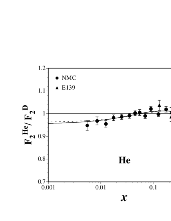
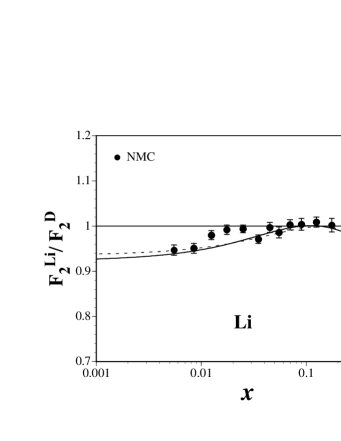
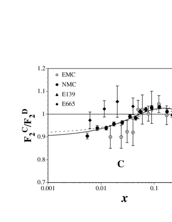
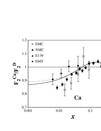
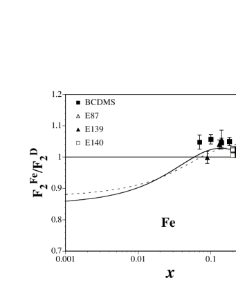
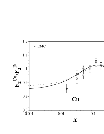
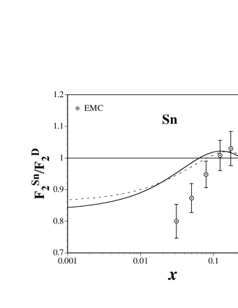
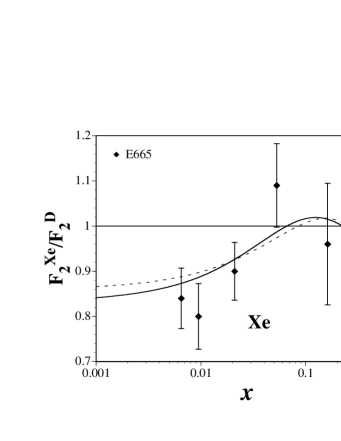
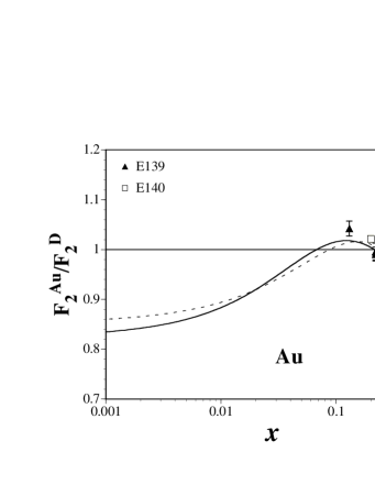
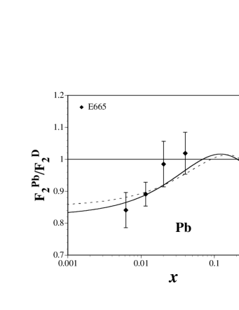
Fitting results are compared with experimental data for all the used nuclear data in Figs. 3$-$16. Obtained optimum parton distributions are used for calculating the curves at $Q^{2}$=5 GeV² in these figure. The dashed and solid curves indicate the ratios in the quadratic and cubic analyses, respectively. The experimental data are taken at various $Q^{2}$ points as shown in Fig. 2, so that the data cannot be compared directly with the curves; nevertheless we can see a general tendency.

Obtained minimum $\chi^{2}$ values are $\chi_{min}^{2}$=583.7 and 546.6 in the quadratic and cubic analyses, respectively, for the 309 total data points. Because the $\chi^{2}$ per degrees of freedom is given by $\chi_{min}^{2}/d.o.f.$=1.93 (quadratic) and 1.82 (cubic), they may not seem to be excellent fits. However, it is partly due to scattered experimental data as it is obvious, for example, from Fig. 10. The data from different experimental groups are scattered particularly in the small $x$ region, and they contribute to $\chi^{2}$ significantly. Therefore, a slightly large $\chi_{min}^{2}$ ($\chi_{min}^{2}/d.o.f.>1$) is unavoidable whatever the analysis method is.

From the figures, we find that the experimental shadowing at small $x<0.05$ and anti-shadowing at $x\sim 0.15$ are generally well reproduced by the analysis. There are slight deviations from the data at medium $x$ for carbon and nitrogen. However, if we try to explain the carbon and nitrogen data at medium $x$, we overestimate the depletion for the beryllium, silver, and gold as obvious from Figs. 7, 13, and 16. The fit is also not excellent for the helium at medium $x$. The reason could be that the helium nucleus is an exceptional tightly-bound system which cannot be explained by the simple $1/A^{1/3}$ behavior.

There are typical differences between the quadratic and cubic curves in Figs. 3$-$16. They are different in the small $x$ region, where there are not so many experimental data. The quadratic curves are above the cubic ones at small $x$ ($0.001<x<0.01$), but they are below in the region $0.03<x<0.14$. Both curves agree well in the larger $x$ region, where there are many experimental data. From these figures, we find that both analyses results are similar except for the minor differences in the small $x$ region.

Table 2: Each $\chi^{2}$ contribution.

nucleus	# of data	$\chi^{2}$ (quad.)	$\chi^{2}$ (cubic)
He	35	55.6	54.5
Li	17	45.6	49.2
Be	17	39.7	38.4
C	43	97.8	88.2
N	9	10.5	10.4
Al	35	38.8	41.4
Ca	33	72.3	69.7
Fe	57	115.7	92.7
Cu	19	13.7	13.6
Ag	7	12.7	11.5
Sn	8	14.8	17.7
Xe	5	3.2	2.4
Au	19	55.5	49.2
Pb	5	7.9	7.6
total	309	583.7	546.6

Each $\chi^{2}$ contribution is listed in Table 2. We notice that the $\chi^{2}$ values per data are especially larger for the carbon, calcium, and gold nuclei than the average. Because the NMC errors are very small, slight deviations from the NMC data produce large $\chi^{2}$ values. For example, the calcium data at $x=0.25$ have peculiar behavior which cannot be reproduced by a smooth $x$ dependent function, yet they have small errors which contribute significantly to the total $\chi^{2}$.

From the cubic $\chi^{2}$ values in Table 2 in comparison with the quadratic ones, we find significant $\chi^{2}$ improvements in carbon, calcium, iron, and gold, however, by sacrificing the $\chi^{2}$ values for lithium, aluminum, and tin. The additional degrees of freedom make it possible to adjust the distribution shapes to the data. There is a 20% $\chi^{2}$ improvement in the iron from the quadratic analysis to the cubic one; however, the difference is not very clear in Fig. 10 within the region where the data exist, except for the $x\sim 0.1$ region.

From Figs. 3$-$16 and Table 2, we find that the analyses with the quadratic and cubic functional types are both successful for reproducing the major experimental properties. It is obvious from the $\chi^{2}$ comparison that the cubic results are better. However, because the $\chi^{2}$ improvement is not very large and both curves look similar in Figs. 3$-$16, both results could be taken as possible nuclear distributions.

IV.2 Obtained parton distributions

Figure 17: Obtained weight functions for the helium, calcium, and gold nuclei in the quadratic analysis. Only the valence up-quark functions are shown as the valence distributions.

Figure 18: Obtained weight functions for the helium, calcium, and gold nuclei in the cubic analysis. Only the valence up-quark functions are shown as the valence distributions.

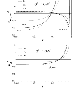
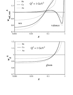
Obtained optimum weight functions in the helium, calcium, and gold nuclei are shown in Figs. 18 and 18 for the quadratic and cubic analyses, respectively. Because valence up- and down-quark functions are the same for isoscalar nuclei and they are very similar in other nuclei, only the valence up-quark functions are shown in these figures.

First, the quadratic results are explained. The valence-quark distributions have depletion at medium $x$ because they should explain the modification of the ratios $R_{F_{2}}^{A}$ at $x\sim 0.6$. Because of the assumed quadratic functional form with the baryon-number constraint, the valence distributions show antishadowing property at small $x$. It indicates 2.6% antishadowing for the calcium nucleus at $x=0.001$. It is noteworthy to reiterate that this quadratic type could not allow a shadowing property for the valence-quark distributions, so that it does not agree with a shadowing prediction, for example, in Ref. fsl although it could agree with a parton-model analysis of Refs. saga ; F3A and also with the one in Ref. kulagin . Next, the antiquark distributions should explain the shadowing of $F_{2}$ at small $x$, so that they also have shadowing property at $x\lesssim 0.07$. The antiquark shadowing is about 20% for the calcium. The antiquark weight functions increase as $x$ becomes larger. They cross the line $w_{\bar{q}}=1$ at $x\sim 0.08$ and continue to increase. The gluon weight functions have similar property to the antiquark functions except that the shadowing is smaller (7% for Ca) and that the crossing point is slightly larger ($x\sim 0.2$). The similar functional form is obtained partly due to the momentum-conservation constraint. The gluon distribution does not contribute significantly in the LO analysis; however, our analysis tends to rule out the gluon antishadowing at small $x$.

We performed the cubic analysis for getting better agreement with the data by the additional adjustable parameters. However, as shown in Fig. 18, the obtained functions are similar to those in Fig. 18 except for the valence functions at small $x$. Now, the valence distributions have freedom to have shadowing or antishadowing property at small $x$. In fact, the results show shadowing for the valence distributions at very small $x$; however, the magnitude is fairly small, 0.1% at $x$=0.001. The bump of $R_{F_{2}}^{A}$ in the region, $0.1<x<0.2$, is explained mainly by the antiquark distributions. This situation is very different, for example, from the picture in Ref. fsl , where the bump is explained mostly by the valence distributions. Of course, the $F_{2}$ data are not enough to separate the valence and sea distributions, so that we should wait for future experimental activities, especially at a neutrino factory sknu , for precise information.

The antiquark weight functions in the cubic analysis are similar to the ones in the quadratic case. We expected a possibility of much wild behavior. For example, it has shadowing at small $x$, antishadowing at $x\sim 0.15$, depletion at medium $x$, and rise at large $x$. However, even if the input antiquark distributions are given by this functional type in our $\chi^{2}$ analysis, they converge to the functions in Fig. 18.

As mentioned in the previous section, the gluon distributions are assumed to be the quadratic functional form even in the “cubic” fit. Therefore, the obtained functions are very similar to the ones in Fig. 18. We also tried the cubic type for the gluon. The additional factor $d_{g}x^{3}$ controls the behavior at large $x$. However, the medium and large $x$ behavior is almost irrelevant for the gluon, especially in the LO analysis of $F_{2}$. Therefore, it is very difficult to control the gluon parameters in a meaningful way within the $\chi^{2}$ analysis. For example, the $\chi^{2}$ fit could produce an unphysical negative gluon distribution at large $x$ if loose bounds are given for the parameters. It is almost meaningless to introduce the additional freedom at large $x$ without the data which could restrict the gluon distributions themselves. This is the reason why we decided to have the quadratic gluon distributions even in the “cubic” analysis.

We find in Figs. 18 and 18 that the variations from the calcium ($A=40$) to gold ($A=197$) are small. Therefore, the obtained parton distributions could be extrapolated into the distributions in a nucleus with a larger mass number ($A>208$), which is outside the analyzed nuclei in this paper.

Figure 19: Weight functions with errors for the calcium in the quadratic analysis. For an isoscalar nucleus like the calcium, the valence up- and down-quark functions are the same.

Figure 20: Weight functions with errors for the calcium in the cubic analysis.

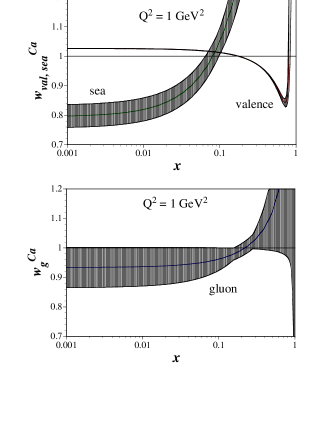
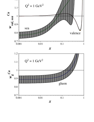
Next, errors are discussed on the obtained weight functions. As an output of the $\chi^{2}$ fit by the Minuit subroutine, the optimum parameters and errors are obtained. The error matrix has a complicated form with nondiagonal elements. It is not straightforward to perform a rigorous error analysis with the complicated error matrix. The project is, for example, in progress as an activity of the Asymmetry Analysis Collaboration (AAC) aac , and there are also recent studies in Ref. error . Here, we employ a simple method which is used for example in Ref. smc . Effects of the Minuit errors on $w_{i}$ are calculated exclusively for each parameter, and then maximum variations are shown as errors in the function $w_{i}$. The calcium results are shown in Figs. 19 and 20 for the quadratic and cubic analyses, respectively. In an isoscalar nucleus like the calcium, the valence up-quark function is the same as the valence down-quark function. The valence-quark functions have some errors around the minimum point at $x\sim 0.7$; however, the small $x$ region is well determined as long as the functional form is fixed. However, there are uncertainties in the small $x$ behavior since both valence functions are different at small $x$ in Figs. 19 and 20. This kind of error, originating from the assumed functional form, is not taken into account in the error bands of these figures.

The antiquark functions have some errors at small $x$; however, they are obviously shadowed at small $x$. The errors and the distribution shapes are very similar at small $x$ in Figs. 19 and 20. Other interesting point is that both errors are very different in the medium $x$ region, $x>0.1$. Therefore, the antiquark weight function cannot be well determined at $x>0.1$, and it depends on the assumed functional form. There should be also differences in the large $x$ region. However, because the antiquark distributions are very small at $x\gtrsim 0.4$ and they do not contribute to $F_{2}$ significantly, the large-$x$ antiquark distributions are not important unless we consider a reaction which is sensitive to them.

As shown in Figs. 19 and 20, the gluon weight functions have large errors in the whole $x$ region. The first reason for the large errors is that the analyses are done in the leading order, and the second is that only $F_{2}$ data are used for the $\chi^{2}$ analyses. Nevertheless, it is interesting to find that the gluon distributions are shadowed at small $x$ even if the errors are taken into account. Next, there is a tendency of increase as $x$ becomes larger. Determination of large-$x$ gluon distributions is not possible in the present analyses. From the simple estimate, we showed the errors in the weight functions. However, these studies are intended to give rough ideas on the errors. In future, we try to investigate a more complete error analysis.

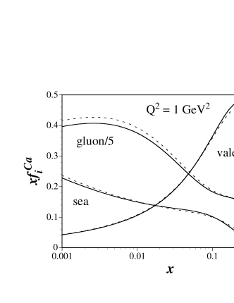
Using the results for the weight functions, we show the parton distributions for the calcium nucleus at $Q^{2}$=1 GeV² in Fig. 21. The dashed and solid curves are the quadratic and cubic analysis results, respectively. From the $F_{2}^{A}$ measurements, the quark distributions are relatively well determined. For determining the gluon distributions and the details of the quark distributions, we need to use other reaction data. Especially, future hadron-collider data should be useful.

Figure 21: Parton distributions for the calcium are shown. The dashed and solid curves indicate the quadratic and cubic results, respectively. For the calcium, the valence up- and down-quark distributions are the same.

From these analyses, we clarified how well the nuclear parton distributions can be determined only by the measurements of the structure functions $F_{2}^{A}$. As mentioned in the introduction, the nuclear parametrization is still premature in the sense that theoretical and experimental efforts are necessary for determining the accurate distributions. As far as the parametrization fit is concerned, much detailed analyses should be done as an extension of our present studies. On the other hand, the authors hope that experimental efforts will be made for probing the valence-quark distributions at small $x$ by a neutrino factory and for finding the antiquark and gluon distributions by hadron colliders such as RHIC.

Our studies should be also important for investigating the parton distributions in the nucleon. As mentioned in Sec. I, nuclear data have been used partially for obtaining the parton distributions in the nucleon. In particular, neutrino data are important for determining the valence-quark distributions; however, the data are taken for example for the iron nucleus. We need to feed back our studies to readjust the distributions in the “nucleon”.

V Practical nuclear parton distributions

The nuclear parton distributions obtained in our analyses could be used for studying other high-energy nuclear reactions. We propose two types of distributions which are obtained in the quadratic and cubic type analyses. Because the $\chi_{min}^{2}$ is smaller for the cubic type, we prefer it to the quadratic type. The distributions are provided either in the analytical form at $Q^{2}$=1 GeV² or in the form of computer subroutines. Although there could exist distributions at $x>1$ in a nucleus, such large $x$ distributions are not provided in our studies as explained in Sec. II.2. The analytical expressions are given in Sec. V.1, the subroutines are explained in Sec. V.2.

V.1 Analytical expressions

The analytical expressions are given at $Q^{2}$=1 GeV². Therefore, one needs to evolve the distributions to a specific $Q^{2}$ point by one’s own evolution code with $\Lambda_{LO}^{MRST}=0.1741$ GeV. If it were the case where $Q^{2}$ dependence can be neglected, one may use the analytical distributions without the evolution. The nuclear distributions should be calculated by Eq. (8) with the obtained weight functions and MRST-LO (central gluon) distributions mrst . However, one should be careful that the antiquark distributions are slightly modified from the original form so as to become flavor symmetric $\bar{q}\equiv Sea(MRST)/6$, because the antiquark flavor asymmetry is not taken into account in our nuclear analyses.

V.1.1 Type I: Cubic fit

We call the cubic distributions type I distributions. The weight functions obtained in the cubic fit are

$$w_{u_{v}} =1+\left(1-\frac{1}{A^{1/3}}\right)$$

$$\ \ \ \ \ \ \ \ \times\frac{a_{u_{v}}(A,Z)+0.6222x-2.858x^{2}+2.557x^{3}}{(1-x)^{0.8107}},$$

$$w_{d_{v}} =1+\left(1-\frac{1}{A^{1/3}}\right)$$

$$\ \ \ \ \ \ \ \ \times\frac{a_{d_{v}}(A,Z)+0.6222x-2.858x^{2}+2.557x^{3}}{(1-x)^{0.8107}},$$

$$w_{\bar{q}} =1+\left(1-\frac{1}{A^{1/3}}\right)$$

$$\ \ \ \ \ \ \ \ \times\frac{-0.3313+6.995x-34.17x^{2}+62.54x^{3}}{1-x},$$

$$w_{g} =1+\left(1-\frac{1}{A^{1/3}}\right)\frac{a_{g}(A,Z)+0.8008x-0.4004x^{2}}{1-x}.$$ (1)

The nuclear dependent constants are listed in Table 3 for the used nuclei. They depend on the mass number $A$ and atomic number $Z$ in general.

Table 3: Obtained parameters $a_{u_{v}}$, $a_{d_{v}}$, and $a_{g}$ for the used nuclei in the cubic analysis.

nucleus	$a_{u_{v}}$	$a_{d_{v}}$	$a_{g}$
D	$-$0.002178	$-$0.002178	$-$0.1560
He	$-$0.002178	$-$0.002178	$-$0.1560
Li	$-$0.002690	$-$0.001716	$-$0.1560
Be	$-$0.002571	$-$0.001815	$-$0.1560
C	$-$0.002178	$-$0.002178	$-$0.1560
N	$-$0.002178	$-$0.002178	$-$0.1560
Al	$-$0.002306	$-$0.002054	$-$0.1560
Ca	$-$0.002178	$-$0.002178	$-$0.1560
Fe	$-$0.002427	$-$0.001941	$-$0.1560
Cu	$-$0.002456	$-$0.001916	$-$0.1560
Ag	$-$0.002610	$-$0.001782	$-$0.1560
Sn	$-$0.002726	$-$0.001686	$-$0.1560
Xe	$-$0.002814	$-$0.001616	$-$0.1560
Au	$-$0.002902	$-$0.001549	$-$0.1560
Pb	$-$0.002955	$-$0.001509	$-$0.1560

As obvious from the table, there are significant nuclear dependence in the parameters $a_{u_{v}}$ and $a_{d_{v}}$. However, the dependence is so small in the parameter $a_{g}$ that it cannot be shown in the table. These parameters are the same for isoscalar nuclei because of the conditions in Eqs. (9), (10), and (11), and this fact is clearly shown in Appendix A. If one would like to have analytical expressions for a nucleus which is not listed in Table 3, there are following two possibilities. The first method is that one calculates $a_{u_{v}}$, $a_{d_{v}}$, and $a_{g}$ so as to satisfy the conditions of nuclear charge, baryon number, and momentum in Eqs. (9), (10), and (11) for one’s chosen nucleus.

For those who think this calculation is tedious, we prepare an alternative method. Using the three conditions, we find that $a_{u_{v}}$, $a_{d_{v}}$, and $a_{g}$ can be expressed in terms of eight integrals, which are nuclear independent, together with $A$ and $Z$. The details of this method are so technical that they are discussed in Appendix A. If one still thinks that these calculations are too much works to do, or if one does not have a $Q^{2}$ evolution subroutine, one had better use computer codes explained in Sec. V.2 for getting numerical values of the parton distributions.

V.1.2 Type II: Quadratic fit

We call the quadratic distributions type II distributions. The weight functions obtained in the quadratic fit are

$$w_{u_{v}} =1+\left(1-\frac{1}{A^{1/3}}\right)\frac{a_{u_{v}}(A,Z)-0.2593\,x+0.2586\,x^{2}}{(1-x)^{2.108}},$$

$$w_{d_{v}} =1+\left(1-\frac{1}{A^{1/3}}\right)\frac{a_{d_{v}}(A,Z)-0.2593\,x+0.2586\,x^{2}}{(1-x)^{2.108}},$$

$$w_{\bar{q}} =1+\left(1-\frac{1}{A^{1/3}}\right)\frac{-0.2900+3.774\,x-2.236\,x^{2}}{1-x},$$

$$w_{g} =1+\left(1-\frac{1}{A^{1/3}}\right)\frac{a_{g}(A,Z)+0.4798\,x-0.2399\,x^{2}}{1-x}.$$ (2)

The nuclear dependent parameters are listed in Table 4. We find that the $A$ dependent variations are very small in these parameters of the quadratic fit. If one needs expressions for other nucleus, one should evaluate $a_{u_{v}}$, $a_{d_{v}}$, and $a_{g}$ as suggested in the type I section.

Table 4: Obtained parameters $a_{u_{v}}$, $a_{d_{v}}$, and $a_{g}$ for the used nuclei in the quadratic analysis.

nucleus	$a_{u_{v}}$	$a_{d_{v}}$	$a_{g}$
D	0.03745	0.03745	$-$0.09391
He	0.03745	0.03745	$-$0.09391
Li	0.03709	0.03776	$-$0.09392
Be	0.03717	0.03770	$-$0.09392
C	0.03745	0.03745	$-$0.09391
N	0.03745	0.03745	$-$0.09391
Al	0.03736	0.03753	$-$0.09391
Ca	0.03745	0.03745	$-$0.09391
Fe	0.03727	0.03761	$-$0.09391
Cu	0.03725	0.03763	$-$0.09391
Ag	0.03714	0.03772	$-$0.09392
Sn	0.03706	0.03778	$-$0.09392
Xe	0.03700	0.03783	$-$0.09393
Au	0.03694	0.03788	$-$0.09394
Pb	0.03690	0.03790	$-$0.09394

V.2 Parton distribution library

If one needs to have nuclear parton distributions in a numerical form at a given $x$ and $Q^{2}$ point, one may use the computer codes in Ref. nucl-lib . Two kinds of subroutines are made. First, there is a subroutine for the used nuclei in this paper. For other nuclei, we prepared the second one.

First, if one wishes to calculate the distributions in the used nuclei: D, ⁴He, Li, Be, C, N, Al, Ca, Fe, Cu, Ag, Sn, Xe, Au, and Pb, one should use the first code. In addition, we prepared the distributions in the nucleon because we modified the MRST antiquark distributions as flavor symmetric in our studies. The kinematical ranges are $10^{-9}\leq x\leq 1$ and $1\ {\rm GeV}^{2}\leq Q^{2}\leq 10^{5}\ {\rm GeV}^{2}$. The variables $x$ and $Q^{2}$ are divided into small steps. Then, a grid data set is prepared for the parton distributions in each nucleus. Because the scaling violation is a rather small effect, a simple linear interpolation in $log\,Q^{2}$ is used for calculating the distributions at a given $Q^{2}$. On the other hand, because the $x$ dependence is more complicated, a cubic Spline interpolation is used for calculating the distributions at a given $x$ point. Running this code, one obtains the distributions, $xu_{v}^{A}$, $xd_{v}^{A}$, $x\bar{q}^{A}$, and $xg^{A}$, for a specified nucleus at a given $x$ and $Q^{2}$ point. Even though the antiquark distributions are flavor symmetric at $Q^{2}$=1 GeV², they are not symmetric at different $Q^{2}$ in the next-to-leading order skpr . However, because such $Q^{2}$ evolution effects do not exist in the leading order, the antiquark distributions are consistently flavor symmetric at any $Q^{2}$.

Second, if one would like to have the distributions in other nucleus, one should use the second code. Here, the analytical expressions in Sec. V.1 are used as the initial distributions. At first, the constants $a_{u_{v}}$, $a_{d_{v}}$, and $a_{g}$ are calculated so as to satisfy the charge, baryon-number, and momentum conditions for a given nucleus with $A$ and $Z$. Then, they are evolved to a requested $x$ and $Q^{2}$ point by the ordinary DGLAP evolution equations in Ref. bf1 . However, one has to be careful about the requested nucleus in the sense that it should not be too far away from the used nuclei. For example, we do not support the distributions in an extremely unstable nucleus with large neutron excess. Strictly speaking, huge nuclei with $A>208$ are also outside our supporting range. However, as obvious from Figs. 18 and 18, the variations of the parton distributions are already very small between the calcium with $A=40$ and gold with $A=197$, so that the extrapolation from $A=208$ to nuclear matter is expected to be reliable. The details of the usage are explained in Ref. nucl-lib .

In the second code, it takes time for getting the results because the $Q^{2}$ evolution calculations consume computing time. It does not matter to calculate the distributions for a few $Q^{2}$ points. However, if one would like to use it frequently, one may try the following. The second code is prepared so that one could create a grid file for a requested nucleus. Then, one can use it in the first code, where the computation is much faster.

VI Summary

We have done the global analyses of existing experimental data on nuclear $F_{2}$ for obtaining optimum parton distributions in nuclei. Assuming a simple yet reasonable overall $A$ dependence, the nuclear parton distributions are expressed in terms of a number of parameters. The quadratic and cubic functional forms are assumed for the $x$ dependence. The parameters have been determined by the $\chi^{2}$ analyses. As a result, we obtained reasonable fit to the measured experimental data of $F_{2}$. The valence-quark distributions are relatively well determined except for the fact that the small $x$ part depends slightly on the assumed functional form. The antiquark distributions are reasonably well determined at small $x$; however, the large $x$ behavior is not obvious from the $F_{2}$ data. The analyses indicated that the gluon distributions are shadowed at small $x$: however, they cannot be well determined by the present $F_{2}$ data, especially in the large $x$ region.

We have proposed two types of nuclear parton distributions which are obtained by the quadratic and cubic type analyses. They are provided either by the analytical expressions at $Q^{2}$=1 GeV² or by the computer programs for calculating them numerically. Our analyses should be important not only for understanding physics mechanisms of nuclear modification but also for applications to heavy-ion physics. Our results could also shed light on an issue of present parton distributions in the nucleon because nuclear data have been partially used in the “nucleon” analysis.

Appendix A Nuclear dependent parameters

From the conditions of nuclear charge, baryon number, and momentum, the nuclear dependent parameters, $a_{u_{v}}$, $a_{d_{v}}$, and $a_{g}$, can be expressed in terms of eight integrals together with $A$ and $Z$. It is the advantage that these integrals are nuclear independent. Therefore, reading the numerical values of the integrals and using the equations in this section, one can easily calculate the values of $a_{u_{v}}$, $a_{d_{v}}$, and $a_{g}$ for any nuclei. The necessary integrals are the following:

$$I_{1} =\int dx\frac{H_{v}(x)}{(1-x)^{\beta_{v}}}\,u_{v}(x),\ \ \ \ I_{2}=\int dx\frac{H_{v}(x)}{(1-x)^{\beta_{v}}}\,d_{v}(x),$$

$$I_{3} =\int dx\frac{1}{(1-x)^{\beta_{v}}}\,u_{v}(x),\ \ \ \ I_{4}=\int dx\frac{1}{(1-x)^{\beta_{v}}}\,d_{v}(x),$$

$$I_{5} =\int dx\frac{x}{(1-x)^{\beta_{v}}}\,u_{v}(x),\ \ \ \ I_{6}=\int dx\frac{x}{(1-x)^{\beta_{v}}}\,d_{v}(x),$$

$$I_{7} =\int dx\,x\,\bigg{[}\,\frac{H_{v}(x)}{(1-x)^{\beta_{v}}}\,\{u_{v}(x)+d_{v}(x)\}$$

$$\ \ \ \ \ \ \ \ \ \ \ \ \ \ \ +\frac{a_{\bar{q}}+H_{\bar{q}}(x)}{1-x}\,6\,\bar{q}(x)+\frac{H_{g}(x)}{1-x}\,g(x)\,\bigg{]},$$

$$I_{8} =\int\frac{x}{1-x}\,g(x).$$ (3)

We should note that the parton distributions in these equations are those in the nucleon. The functions $H_{i}(x)$ are the one given in Eq. (8). The integral values are numerically given in Table 5.

Table 5: Values of the integrals are given.

Integral	Type I	Type II
$I_{1}$	$-$0.0007990	$-$0.1474
$I_{2}$	0.008540	$-$0.05297
$I_{3}$	2.406	3.768
$I_{4}$	1.148	1.583
$I_{5}$	0.4777	1.157
$I_{6}$	0.1772	0.3629
$I_{7}$	0.08326	$-$0.007650
$I_{8}$	0.5246	0.5246

Using these integrals, we can express the nuclear dependent parameters as

$$a_{u_{v}}(A,Z) =-\frac{ZI_{1}+(A-Z)I_{2}}{ZI_{3}+(A-Z)I_{4}},$$

$$a_{d_{v}}(A,Z) =-\frac{ZI_{2}+(A-Z)I_{1}}{ZI_{4}+(A-Z)I_{3}},$$

$$a_{g}(A,Z) =-\frac{1}{I_{8}}\,\bigg{[}\,a_{u_{v}}(A,Z)\left\{\frac{Z}{A}I_{5}+\left(1-\frac{Z}{A}\right)I_{6}\right\}$$

$$\!\!\!\!\!\!\!+a_{d_{v}}(A,Z)\left\{\frac{Z}{A}I_{6}+\left(1-\frac{Z}{A}\right)I_{5}\right\}+I_{7}\,\bigg{]}.$$ (4)

From Table 5 and Eq. (4), it is possible to calculate the parton distributions in any nucleus. However, we recommend to use our results for a nucleus which is rather close to the analyzed nuclei.

References

- (1) H. L. Lai et. al. (CTEQ Collaboration), Eur. Phys. J. C12, 375 (2000).
- (2) M. Glück, E. Reya, and A. Vogt, Eur. Phys. J. C5, 461 (1998).
- (3) A. D. Martin, R. G. Roberts, W. J. Stirling, and R. S. Thorne, Eur. Phys. J. C14, 133 (2000).
- (4) Y. Goto et. al. (Asymmetry Analysis Collaboration (AAC)), Phys. Rev. D62, 034017 (2000). The AAC library is available at http://spin.riken.bnl.gov/aac. H. Kobayashi et al., error analysis in progress.
- (5) For a summary, see D. F. Geesaman, K. Saito, and A. W. Thomas, Ann. Rev. Nucl. Part. Sci. 45, 337 (1995).
- (6) S. Kumano, Phys. Rev. C48, 2016 (1993); S. Kumano and K. Umekawa, SAGA-HE-130-98 (hep-ph/9803359).
- (7) K. J. Eskola, V. J. Kolhinen, and P. V. Ruuskanen, Nucl. Phys. B535, 351 (1998).
- (8) A preliminary version is reported in M. Hirai, S. Kumano, and M. Miyama, invited talk at the international symposium on nuclear physics, Mumbai, India, Dec. 1822, 2000 (see http://www-hs.phys.saga-u.ac.jp/talk00.html), preprint SAGA-HE-171-01, to be published in the proceedings.
- (9) S. Kumano, invited talk at the KEK workshop on neutrino factory, KEK, Japan, Sept. 1314, 2000, see http://www-hs.phys.saga-u.ac.jp/talk00.html for the presentation.
- (10) I. Sick and D. Day, Phys. Lett. B274, 16 (1992).
- (11) M. Miyama and S. Kumano, Comput. Phys. Commun. 94, 185 (1996).
- (12) A. H. Mueller and J. Qiu, Nucl. Phys. B268, 427 (1986).
- (13) R. Kobayashi, S. Kumano, and M. Miyama, Phys. Lett. B354, 465 (1995).
- (14) J. Ashman et al. (European Muon Collaboration (EMC)), Phys. Lett. B202, 603 (1988).
- (15) M. Arneodo et al. (EMC), Nucl. Phys. B333, 1 (1990).
- (16) J. Ashman et al. (EMC), Z. Phys. C57, 211 (1993).
- (17) A. Bodek et al. (SLAC-E87 Collaboration), Phys. Rev. Lett. 50, 1431 (1983).
- (18) A. Bodek et al. (SLAC-E49), Phys. Rev. Lett. 51, 534 (1983).
- (19) S. Dasu et al. (SLAC-E140), Phys. Rev. Lett. 60, 2591 (1988).
- (20) J. Gomez et al. (SLAC-E139), Phys. Rev. D49, 4348 (1994).
- (21) G. Bari et al. (BCDMS Collaboration), Phys. Lett. 163B, 282 (1985).
- (22) A. C. Benvenuti et al. (BCDMS), Phys. Lett. B189, 483 (1987).
- (23) P. Amaudruz et al. (New Muon Collaboration (NMC)), Nucl. Phys. B441, 3 (1995); M. Arneodo et al. (NMC), Nucl. Phys. B441, 12 (1995).
- (24) M. R. Adams et al. (FNAL-E665 Collaboration), Phys. Rev. Lett. 68, 3266 (1992); H. Schellman, personal communication (2000).
- (25) M. R. Adams et al. (E665), Z. Phys. C67, 403 (1995).
- (26) M. Arneodo, A. Bialas, M. W. Krasny, T. Sloan, and M. Strikman, hep-ph/9610423.
- (27) See http://quark.phy.bnl.gov/~raju/eRHIC.html.
- (28) S. Kumano, Phys. Rep. 303, 183 (1998); J.-C. Peng and G. T. Garvey, hep-ph/9912370.
- (29) S. Kumano, Phys. Lett. B342, 339 (1995).
- (30) The P906 Collaboration, proposal for Drell-Yan measurements at the FNAL Main Injector (1999).
- (31) A. D. Martin, R. G. Roberts, W. J. Stirling, and R. S. Thorne, Eur. Phys. J. C4, 463 (1998). Analytical expressions of the MRST-LO distributions at =1 GeV2 are provided by R. G. Roberts and W. J. Stirling through personal communications.
- (32) F. James, CERN Program Library Long Writeup D506 (unpublished).
- (33) L. L. Frankfurt, M. I. Strikman, and S. Liuti, Phys. Rev. Lett. 65, 1725 (1990).
- (34) S. A. Kulagin, Nucl. Phys. A640, 435 (1998).
- (35) J. Pumplin et al., hep-ph/0101032.
- (36) Spin Muon Collaboration (SMC), B. Adeva et al., Phys. Rev. D58, 112002 (1998).
- (37) Nuclear parton-distribution subroutines could be obtained at the web site: http://www-hs.phys.saga-u.ac.jp.