THE MESON MASS SPECTRUM FROM A SYSTEMATICALLY RENORMALIZED LIGHT-FRONT HAMILTONIAN

Abstract

We extend a systematic renormalization procedure for quantum field theory to include particle masses and present several applications. We use a Hamiltonian formulation and light-front quantization because this may produce a convergent Fock-space expansion. The QCD Hamiltonian is systematically renormalized to second order in the strong coupling and the Fock-space expansion is truncated to lowest order to produce a finite-dimensional Hamiltonian matrix. The renormalized Hamiltonian is used to calculate the spectra of the $b\bar{b}$ and $c\bar{c}$ mesons as a lowest-order test of our procedure for full QCD.

The analytic determination of the renormalized Hamiltonian matrix generates expressions that must be numerically integrated to generate quantitative results. The efficiency of the numerical calculation depends on how well the basis functions can approximate the real state. We examine the effectiveness of using Basis-Splines (B-Splines) to represent QCD states. After briefly describing these functions, we test them using the one- and two-dimensional harmonic oscillator problems. We test their ability to represent realistic wavefunctions by using them to find the glueball mass spectrum.

An efficient algorithm for numerically calculating the matrix elements in the glueball and meson problems is necessary because the calculation is numerically intensive. We describe our algorithm and discuss its parallel-cpu implementation.

For Nikki and David

March 15, 1973Born – Mayfield Heights, Ohio 1995B.S. Physics, The University of California, Davis 1998M.S. Physics, The Ohio State University 1995–presentGraduate Teaching and Research Associate, The Ohio State University

“Optimization of Fullerene Yields in a Plasma Arc Reactor;” P.E. Anderson, T. T. Anderson, P. L. Dyer, J. W. Dykes, S. H. Irons, C. A. Smith, R. D. Kylin, P. Klavins, J. Z. Liu, and R. N. Shelton, in the proceedings on Recent Advances in the Chemistry and Physics of Fullerenes and Related Materials, Karl M. Kadish and Rodney S. Ruoff, eds. (The Electrochemical Society, Inc., 1994) “Systematic Renormalization in Hamiltonian Light-Front Field Theory: The Massive Generalization;” Roger D. Kylin, Brent H. Allen, and Robert J. Perry Phys. Rev. D 60 (1999) 067704, hep-th/9812080.

Physics

Chapter 0 Introduction

The physics of quarks and gluons is described by quantum chromodynamics (QCD), which is universally believed to be the fundamental theory of the strong interaction. High energy QCD systems (small spatial separations) behave as though the particles interact weakly (asymptotic freedom). Low energy systems (large spatial separations) interact so strongly that it is not possible to isolate a quark or gluon (confinement). The physics in the confining and asymptotically free systems is so different that it is has not yet been possible to write down a solution to QCD that is valid in both regimes. Historically, difficult theories like QCD are first solved for simple systems. Solving these systems provides an initial test of the theory before more complex systems are attacked and a development ground for new techniques.

Heavy quark bound states are relatively simple because the large quark mass dominates the spectrum and the average separation of quarks and gluons is small, so that dynamics are largely described by asymptotic freedom. This also allows the interactions to be treated nonrelativistically [1, 2, 3, 4, 5]. Techniques that have been applied to the heavy quark system include nonrelativistic potential models and nonrelativistic QCD (NRQCD). Potential models [6, 7] obtain good predictive power by approximating the interaction between particles using nonrelativistic potentials, although these potentials are not directly obtained from QCD. Predictions include the $\Upsilon$/$\Upsilon^{\prime}$ splitting [8], spin-splitting, transition rates and hadronic transitions [7].

NRQCD uses a nonrelativistic expansion of QCD operators to generate an approximate Lagrangian that can be systematically improved [9]. Heavy-quark spectroscopy can be determined on the lattice [10], which can then be used to determine the strong coupling constant, which is important because the coupling can be compared to perturbative results and could reveal the existence of new physics [12]. Both potential models and NRQCD have proven to be predictive theories for nonrelativistic systems. Despite both theories being improvable, a relativistic treatment of QCD is necessary to treat systems of lighter quarks.

There are many problems one must solve (or circumvent) to solve full QCD. In Euclidean or equal-time coordinates vacuum fluctuations prevent using a constituent picture for low energy hadrons. Also, since QCD is a field theory, there are divergences that must be regulated, often breaking symmetries. Any solution to QCD will require the use of renormalization to remove the dependence on the regulator and to restore broken symmetries.

Hadrons are composed of at least two (meson) or three (baryon) quarks. The quarks are bound by the strong force through the exchange of color-charged gluons, which are in turn bound together by the same mechanism. Hadronic bound states (and glueball states) are color singlets; there is no net color. As quarks in a baryon are separated, the energy of the system increases, eventually allowing the creation of new quark-antiquark pairs. These pairs form bound states with the separated quarks, preventing the isolation of any individual quark. If we consider low-energy bound states, the particles interact weakly and we may be able to make a constituent approximation. However in a standard equal-time picture Heisenberg’s uncertainty principle allows quark-antiquark pairs to fluctuate out of the vacuum. These quarks can then interact with any hadronic bound states, preventing the state from being successfully represented by two or three quarks. Moreover, these vacuum fluctuations are usually thought to be critical for strong interactions.

We would like to derive a constituent picture for mesons from QCD, with mesonic states and masses determined by a Schrödinger equation:

$$H|\Psi\rangle=E|\Psi\rangle,$$ (1)

where we can approximate the eigenstate with a truncated Fock-space expansion,

$$|\Psi\rangle=\phi_{q\bar{q}}|q\bar{q}\rangle+\phi_{q\bar{q}g}|q\bar{q}g\rangle+\cdot\cdot\cdot.$$ (2)

$E$ is the energy eigenvalue of the state $|\Psi\rangle$ and we use shorthand notation for the Fock states where $q$ is a quark, $\bar{q}$ an antiquark, and $g$ is a gluon. Unfortunately a Fock-space expansion is not usually thought to be practical, because the complicated equal-time vacuum forces bound-states to contain an infinite number of particles that are part of the physical vacuum on which hadrons are built. It may be possible, however, to obtain a convergent Fock-space expansion if we work in light-front coordinates because the free energy of a state increases at least like the number of particles squared (Sec. 1). This means all states with many particles are high-energy states. Inspired by the work of Dyson [13], Wilson [14], Głazek and Wilson [15], and Wegner [16], significant work has been done to perturbatively derive light-front Hamiltonians in the full Fock-space, neglecting zero modes [3, 4, 5, 17, 18, 19, 20, 21, 22, 23, 24].

Local interactions in a field theory couple states with arbitrarily large differences in free energy, which will invalidate our Fock-space expansion if we can not decouple high-energy states from low-energy states. One way we can force high-energy states to decouple from low-energy states is to simply truncate the Fock-space expansion. The truncated states can be important, and their removal may discard important physics. We can retain all of the physics if we place a cutoff on change in invariant mass between states, and then use a similarity transformation [15, 16] to map the effects from mixing of low- and high-energy states to interactions involving only low-energy states.

The importance of high-energy states can be appreciated by considering the second-order perturbation theory correction to a free energy:

$$\delta E_{n}=\sum_{m\neq n}^{N}\frac{\left|\langle m\left|V\right|n\rangle\right|^{2}}{\langle m\left|H_{0}\right|m\rangle-\langle n\left|H_{0}\right|n\rangle}.$$ (3)

The sum can diverge as $N\rightarrow\infty$ if the matrix elements between states with large differences in energy do not fall off sufficiently rapidly. We regularize the theory by implementing a gaussian cutoff on interactions between states with differing free invariant masses. This cutoff serves two purposes. It makes perturbative corrections like Eq. (3) finite and it reduces the coupling between states with large differences in invariant mass, which further helps justify our Fock-space expansion by reducing the importance of high-energy physics for low-energy states.

The cutoff we use violates Lorentz covariance and gauge invariance, so we can not renormalize the Hamiltonian exclusively through the redefinition of masses and canonical couplings. Renormalization must be completed by requiring the Hamiltonian to produce cutoff-independent physical quantities and by requiring it to obey the physical principles of the theory that are not violated by the cutoff. These requirements, and the assumption that this can be done perturbatively, are sufficient to determine the Hamiltonian so that it will give results consistent with all the physical principles of the theory, even those violated by the cutoff. The most powerful characteristic of this approach is that it systematically “repairs” the theory and requires only the fundamental parameters of the canonical Hamiltonian.

Recently, Allen [25, 26, 27] derived recursion relations that systematically determine the Hamiltonian for massless theories order by order in the coupling and he applied this method to pure-glue QCD. In this dissertation we extend the recursion relations to full QCD and present three applications. We first show how matrix elements of the renormalized Hamiltonian are calculated with our extension of the method, which has been published in [28]. Secondly we apply new numerical methods to verify Allen’s previous glueball spectrum calculation [26, 27]. The final application uses these numerical methods to calculate heavy quarkonia ($q\bar{q}$) spectra.

In light-front field theory the Hamiltonian is trivially related to the invariant mass operator (IMO). The IMO is a natural operator to use because it is boost and rotationally invariant (although rotational invariance is realized dynamically). We calculate the IMO in this dissertation, but refer to it as the Hamiltonian throughout since it governs the time evolution of all states.

The Hamiltonian matrix is calculated analytically to ${\cal O}(\alpha_{s})$ in a plane-wave basis. We then calculate the matrix elements in a basis we choose to approximate the real meson states (i.e., eigenstates of the Hamiltonian). The real meson states are approximated by the first term in a Fock-space expansion, quark-antiquark pairs. Solving the eigensystem gives the invariant masses (eigenvalues) of the system and the coefficients (eigenvectors) needed to build the eigenstates from the basis functions.

The numerical calculation of the Hamiltonian matrix requires us to choose a set of basis functions to approximate the real states. We use Basis-splines (B-splines) to represent the longitudinal and transverse momentum states. Although their derivation from mathematical first principles is non-trivial, their benefit is easily understood. First, B-splines do not oscillate, so they do not add extra oscillations to the function that must be integrated to determine each matrix element. Second, each spline has only a limited spatial overlap with the other splines; thus, there can be a significant number of matrix elements that vanish if the interactions are local because the basis functions do not overlap.

The most substantial drawback to using B-splines is that they are non-orthogonal. This means that an overlap matrix must be calculated to solve Schrödinger’s equation. The main inconvenience is that a general eigensystem problem must be solved and efficient methods that compute only low-lying eigenvalues can not be used.

The numerical calculation of the Hamiltonian matrix is very cpu-intensive because each matrix element includes a five-dimensional integral. Unfortunately one can not know ahead of time how accurately each matrix element must be calculated. For instance, if all matrix elements are calculated to the same precision, much computer time is wasted because all elements are not equally important when determining the low-lying eigenvalues. With no unambiguous method to determine the relative importance of various matrix elements, there is also no obvious algorithm to solve the problem efficiently. Fortunately each matrix element can be calculated independently, so most algorithms can be executed in a parallel computing environment.

In Chapter 1 we discuss our motivation for using light-front coordinates and our choice of regularization and renormalization techniques. We then review a recent technique that builds on previous work, systematically determining the renormalized Hamiltonian for massless theories, and discuss how this method is generalized to theories with massive particles. We conclude Chapter 1 by listing which terms in the Hamiltonian are needed for an ${\cal O}(\alpha)$ calculation, followed by a discussion of how these terms are combined to explicitly cancel light-front divergences.

We present B-splines and show some simple applications in Chapter 2. In Chapter 5 we introduce the basis used to represent the real meson states. This basis is tested by computing the glueball mass spectrum in Section 8.

The matrix elements of the Hamiltonian are presented in Chapters 3, 4, and 6. Chapter 3 presents some matrix elements of the full Hamiltonian in a plane wave basis. The matrix elements of the second-order renormalized Hamiltonian in a plane wave basis are derived in Chapter 4. Finally the matrix elements of the Hamiltonian in the approximate-state basis are given in Chapter 6.

Although there is a lot of analytic work required to solve this problem, quantitative results can only be obtained after applying numerical methods to attack the problem. We discuss some of the numerical considerations when deriving the matrix elements and describe the general algorithm and how it is parallelized in Chapter 7.

Finally, we present our analysis of our numerical methods and the calculation of the meson spectrum in Chapter 8. We make concluding remarks in Chapter 9.

This dissertation builds upon previous work and applies it to a familiar problem using numerical techniques that may be similar to other calculations unknown to the author. We believe the following parts of this calculation are original work:

• We included masses in Renormalization Group calculations using the method in [18].

• Calculation of the renormalized light-front QCD Hamiltonian to ${\cal O}(\alpha)$ using the renormalization methods from [17, 18, 25].

• Use of B-spline basis function to calculate the glueball mass spectrum.

• Numerical calculation of the heavy meson mass spectrum for our renormalized QCD Hamiltonian.

• Development of an efficient algorithm to calculate the Hamiltonian matrix.

Chapter 1 Motivations and Formalism Overview

In this chapter we motivate and give an overview of our method. This includes a discussion of light-front coordinates as well as discussions about regularization and renormalization. We then discuss a recent development that systematically determines the renormalized Hamiltonian by requiring it to produce cutoff-independent results and to obey all physical principles not violated by the cutoff [25, 26, 27]. We then review the generalization to include massive particles from [28]. In Section 6 we list all of the diagrams that contribute to the second-order Hamiltonian. Finally we describe how these diagrams are combined to explicitly cancel the light-front divergences.

This chapter is intended to give a good understanding of the entire approach without saturating the reader with too many details, which can be found in the references.

1 Light-Front Coordinates

Light-front coordinates may be considered a rotation of equal-time coordinates such that light-front time is along the forward light-cone (See Fig 1).

Figure 1: Light-from coordinates in $3+1$ dimensions. $x^{+}$ and $x^{-}$, the light-front time and longitudinal space components are a linear combination of the equal-time 3-direction and time.

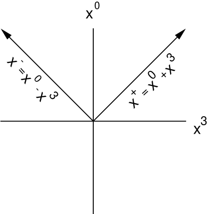
Explicitly we write the light-front time coordinate:

$$x^{+}=x^{0}+x^{3},$$ (1)

and the light-front longitudinal space coordinate as:

$$x^{-}=x^{0}-x^{3}.$$ (2)

The scalar product of light-front vectors is:

$$a\cdot b=\frac{1}{2}a^{+}b^{-}+\frac{1}{2}a^{-}b^{+}-{\mathrm{\bf a}}_{\perp}\cdot{\mathrm{\bf b}}_{\perp},$$ (3)

where ${\mathrm{\bf a}}_{\perp}$ and ${\mathrm{\bf b}}_{\perp}$ are the transverse components. This shows that the light-front energy, which is conjugate to light-front time, is $p^{-}$ and the longitudinal momentum is $p^{+}$. An on-mass-shell particle obeys $p^{0}\geq p^{3}$ which implies $p^{+}\geq 0$. Finally a free particle of mass $m$ has the light-front energy

$$p^{-}=\frac{{\mathrm{\bf p}}^{2}_{\perp}+m^{2}}{p^{+}}.$$ (4)

The light-front energy is finite unless the longitudinal momentum is zero. The study of these infinite-energy zero modes is rich. Since they are infinite energy modes we discard them in our approach, although their effects will need to be added to the Hamiltonian. Using the light-front dispersion relation we can write the free energy of a state as:

$$P^{-}=\frac{1}{P^{+}}\sum_{i}^{\mathrm{N}}\frac{\mathrm{{\bf p}}^{2}_{i\perp}+m_{i}^{2}}{x_{i}},$$ (5)

where $P^{+}$ is the total longitudinal momentum of the state, N is the number of particles in the state, the index $i$ refers to each particle in the state, and $x_{i}$ is the $i^{th}$ particle’s longitudinal momentum fraction. If we assume all particles in the state have similar masses and transverse momenta, we can write the energy as:

$$P^{-}\sim\frac{(\mathrm{{\bf p}}^{2}_{\perp}+m^{2})_{typical}}{P^{+}}\sum_{i}^{\mathrm{N}}\frac{1}{x_{i}}.$$ (6)

The free energy is minimized if the particles equally share the longitudinal momentum ($x_{i}=\frac{1}{N}$). This means the minimum free energy of a light-front state behaves like:

$$P^{-}_{\mathrm{min.}}\sim N^{2}(\mathrm{{\bf p}}^{2}_{\perp}+m^{2})_{typical}.$$ (7)

Since the energy of the state increases like the number of particles squared, a Fock-space expansion may be justified.

See appendix 10 for a complete presentation of the light-front formalism used in this paper.

2 Regularization

In the next two sections we discuss the procedure we use to regulate and renormalize the Hamiltonian. Our discussion follows the one in [18] and we do not cite each instance an argument from this reference is used.

If particle number is not conserved in a theory, there can be arbitrarily many particles in a state. In addition each state can be coupled to every other state through a matrix element of the Hamiltonian, yielding a Hamiltonian with an infinite number of matrix elements. We must regularize the Hamiltonian so it is finite dimensional. We could simply limit the number of particles in a state. This type of truncation is called a Tamm-Dancoff truncation [30, 31, 32] and suffers from divergent sensitivity to the precise form of the truncation, and removing this sensitivity can be as hard as solving the full theory.

Consider a Hamiltonian that can be written as;

$$H=H_{0}+V,$$ (8)

where V can be considered a perturbation. To second order in perturbation theory, the energy of a state $|n\rangle$, is given by:

$$E_{n}=\langle n\left|H_{0}\right|n\rangle+\langle n\left|V\right|n\rangle-\sum_{m\neq n}\frac{\left|\langle m\left|V\right|n\rangle\right|^{2}}{\langle m\left|H_{0}\right|m\rangle-\langle n\left|H_{0}\right|n\rangle}.$$ (9)

If this sum is over a finite number of states, and the matrix elements are finite, the sum will be finite. However, if the sum is over an infinite number of states, the sum may not converge if the matrix elements between states do not fall off fast enough. One way we can ensure this sum is finite is to place a cutoff on the Hamiltonian that reduces the coupling between states with arbitrarily large differences in free energy.

Since perturbative calculations can only lead to reasonable results when the cutoff is a function of the free energy variables and we want a cutoff that will also prevent small energy denominators, we choose to place a smooth cutoff on change in invariant-mass (free energy) between the final and initial states [Eq. (17)]. Like all cutoffs, this violates Lorentz covariance and gauge invariance. However, it is invariant under boosts and rotations about the 3-axis.

The light-front dispersion relation shows that the energy of a state rapidly increases with the number of particles, and the cutoff reduces the coupling between high- and low-energy states. These two facts support the use of a Fock-space expansion.

3 Renormalization

We regulate the Hamiltonian by applying a smooth cutoff on change in invariant-mass between the final and initial states. This introduces cutoff dependence in the Hamiltonian, and it breaks Lorentz covariance and gauge invariance. We restrict the form of the Hamiltonian by requiring it to obey all physical principles unviolated by the cutoff and use the similarity renormalization scheme to perturbatively remove the cutoff dependence. An ${\cal O}(\alpha)$ perturbative renormalization of the regularized Hamiltonian does three things. It removes cutoff dependence and restores broken symmetries to ${\cal O}(\alpha)$.

For notational consistency with Ref. [27] (which we follow in this section) we remind the reader that if we neglect the total transverse momentum of a system, the Hamiltonian is trivially related to the Invariant Mass Operator (IMO) by:

$${\cal M}^{2}={\cal P}^{+}{\cal H}.$$ (10)

We split the IMO into free and interacting parts:

$${\cal M}^{2}(\Lambda)={\cal M}^{2}_{\mathrm{free}}+{\cal M}^{2}_{\mathrm{int}}(\Lambda).$$ (11)

The IMO will produce cutoff independent results if it is unitarily equivalent to itself with an infinite cutoff and satisfies the relation:

$${\cal M}^{2}(\Lambda)=U(\Lambda,\Lambda^{\prime}){\cal M}^{2}(\Lambda^{\prime})U^{\dagger}(\Lambda,\Lambda^{\prime}),$$ (12)

where $U$ is a unitary operator that reduces the cutoff from $\Lambda^{\prime}$ to $\Lambda$. The transformation, which is a simplified version of the one introduced by Wegner [16], is determined by the differential equation:

$$\frac{dU(\Lambda,\Lambda^{\prime})}{d(\Lambda^{-4})}=T(\Lambda)U(\Lambda,\Lambda^{\prime}),$$ (13)

with the boundary condition:

$$U(\Lambda,\Lambda)=1.$$ (14)

We treat the free part of the IMO (${\cal M}^{2}_{\mathrm{free}}$) nonperturbatively and use:

$$T(\Lambda)=\left[{\cal M}^{2}_{\mathrm{free}},{\cal M}^{2}(\Lambda)\right].$$ (15)

If we can determine $T(\Lambda)$, and therefore $U(\Lambda,\Lambda^{\prime})$, then we can use the perturbative transformation repeatedly to lower the cutoff as long as the couplings are not too large. We can choose the initial cutoff to be as large as we want assuming the couplings in the large cutoff limit do not grow, which is true in an asymptotically free theory. This implies that ${\cal M}^{2}(\Lambda)$ is unitarily equivalent to $\lim_{\Lambda\rightarrow\infty}{\cal M}^{2}(\Lambda)$, the IMO with no cutoff. Thus ${\cal M}^{2}(\Lambda)$ will give cutoff-independent results.

We continue with the discussion of the exact form of the transformation and how we add restrictions from unviolated physical principles to fix the form of the renormalized Hamiltonian after more notation has been introduced in Section 4.

4 Review of the Systematic Approach

In this section we introduce more of the notation developed in Refs. [25, 26, 27] and outline the method to systematically determine the renormalized Hamiltonian. Formalism that is necessary for a detailed understanding of this method but that we do not repeat in this paper can be found in this earlier work.

We want to find the regulated invariant-mass operator, ${\cal M}^{2}(g_{{}_{\Lambda}},m,\Lambda)$, which is trivially related to the Hamiltonian. It can be split into a free part (which contains implicit mass dependence) and an interacting part:

$${\cal M}^{2}(g_{{}_{\Lambda}},m,\Lambda)={\cal M}^{2}_{\mathrm{free}}(m)+{\cal M}_{\mathrm{int}}^{2}(g_{{}_{\Lambda}},m,\Lambda).$$ (16)

Since the method treats ${\cal M}_{\mathrm{int}}^{2}(g_{{}_{\Lambda}},m,\Lambda)$ perturbatively, we put the particle-mass term in ${\cal M}_{\mathrm{free}}^{2}(m)$, to treat it non-perturbatively; however, ${\cal M}_{\mathrm{int}}^{2}(g_{{}_{\Lambda}},m,\Lambda)$ will still have mass dependence. The matrix elements of ${\cal M}^{2}(g_{{}_{\Lambda}},m,\Lambda)$ are written

$$\langle F|{\cal M}^{2}(g_{{}_{\Lambda}},m,\Lambda)|I\rangle = \langle F|{\cal M}_{\mathrm{free}}^{2}(m)|I\rangle+\langle F|{\cal M}_{\mathrm{int}}^{2}(g_{{}_{\Lambda}},m,\Lambda)|I\rangle$$ (17)

$$= M^{2}_{F}\langle F|I\rangle+e^{-\frac{\Delta^{2}_{FI}}{\Lambda^{4}}}\langle F|V(g_{{}_{\Lambda}},m,\Lambda)|I\rangle,$$

where $|F\rangle$ and $|I\rangle$ are eigenstates of the free invariant-mass operator with eigenvalues $M_{F}^{2}$ and $M_{I}^{2}$, and $\Delta_{FI}$ is the difference of these eigenvalues. $V(g_{{}_{\Lambda}},m,\Lambda)$ is the interacting part of the invariant-mass operator with the Gaussian cutoff factor removed and is called the “reduced interaction.” The Gaussian cutoff on change in invariant-mass is what regulates the theory (Sec. 2) and it has no effect on the free part of the Hamiltonian.

We expand $V(g_{{}_{\Lambda}},m,\Lambda)$ in powers of the running coupling, $g_{{}_{\Lambda}}$:

$$V(g_{{}_{\Lambda}},m,\Lambda)=\sum_{r=1}^{\infty}g_{{}_{\Lambda}}^{r}V^{(r)}(m,\Lambda),$$ (18)

where $V^{(1)}$ is the canonical interaction and the $V^{(r\geq 2)}(m,\Lambda)$’s are non-canonical interactions in the scalar theory. These non-canonical operators can be thought of as counterterms in a traditional approach. Note that $g_{{}_{\Lambda}}$ implicitly depends on $m$. The assumption that this expansion exists is equivalent to a restricted coupling coherence [33]. We now continue the discussion of the unitary transformation described in Sec. 3.

Allen shows in [27] that the perturbative version of the unitary transformation that lowers the cutoff [derived from Eq. (12)] is:

$$V(\Lambda)-V(\Lambda^{\prime})=\delta V,$$ (19)

where $\delta V$ is the change in the reduced reaction and is a function of both $\Lambda$ and $\Lambda^{\prime}$. Since the free part of the Hamiltonian is independent of the cutoff, calculating $\delta V$ gives us the change in the Hamiltonian when lowering the cutoff from $\Lambda^{\prime}$ to $\Lambda$. The matrix elements of $\delta V$ are found to be:

$$\left<F\right|\delta V\left|I\right> =\frac{1}{2}\sum_{K}\left<F\right|V(\Lambda^{\prime})\left|K\right>\left<K\right|V(\Lambda^{\prime})\left|I\right>T_{2}^{(\Lambda,\Lambda^{\prime})}(F,K,I)$$ (20)

$$+\frac{1}{4}\sum_{K,L}\left<F\right|V(\Lambda^{\prime})\left|K\right>\left<K\right|V(\Lambda^{\prime})\left|L\right>\left<L\right|V(\Lambda^{\prime})\left|I\right>T_{3}^{(\Lambda,\Lambda^{\prime})}(F,K,L,I)$$

$$+{\cal O}\left(\left[V(\Lambda^{\prime})\right]^{4}\right),$$

where the sums are over complete sets of states. $T_{2}^{(\Lambda,\Lambda^{\prime})}(F,K,I)$ and $T_{3}^{(\Lambda,\Lambda^{\prime})}(F,K,L,I)$ are:

$$T_{2}^{(\Lambda,\Lambda^{\prime})}(F,K,I) = \left(\frac{1}{\Delta_{FK}}-\frac{1}{\Delta_{KI}}\right)\left(e^{2\Lambda^{\prime-4}\Delta_{FK}\Delta_{KI}}-e^{2\Lambda^{-4}\Delta_{FK}\Delta_{KI}}\right),$$ (21)

and

$$T_{3}^{(\Lambda,\Lambda^{\prime})}(F,K,L,I)=$$

$$\hskip 28.45274pt\left(\frac{1}{\Delta_{KL}}-\frac{1}{\Delta_{LI}}\right)\left(\frac{1}{\Delta_{KI}}-\frac{1}{\Delta_{FK}}\right)$$

$$\hskip 56.9055pt\times e^{2\Lambda^{\prime-4}\Delta_{KL}\Delta_{LI}}\left(e^{2\Lambda^{-4}\Delta_{FK}\Delta_{KI}}-e^{2\Lambda^{\prime-4}\Delta_{FK}\Delta_{KI}}\right)$$

$$\hskip 28.45274pt+\left(\frac{1}{\Delta_{KL}}-\frac{1}{\Delta_{LI}}\right)\left(\frac{\Delta_{FK}+\Delta_{IK}}{\Delta_{KL}\Delta_{LI}+\Delta_{FK}\Delta_{KI}}\right)$$

$$\hskip 56.9055pt\times\left(e^{2\Lambda^{\prime-4}(\Delta_{FK}\Delta_{KI}+\Delta_{KL}\Delta_{LI})}-e^{2\Lambda^{-4}(\Delta_{FK}\Delta_{KI}+\Delta_{KL}\Delta_{LI})}\right)$$

$$\hskip 28.45274pt+\left(\frac{1}{\Delta_{FK}}-\frac{1}{\Delta_{KL}}\right)\left(\frac{1}{\Delta_{LI}}-\frac{1}{\Delta_{FL}}\right)$$

$$\hskip 56.9055pt\times e^{2\Lambda^{\prime-4}\Delta_{FK}\Delta_{KL}}\left(e^{2\Lambda^{-4}\Delta_{FL}\Delta_{LI}}-e^{2\Lambda^{\prime-4}\Delta_{FL}\Delta_{LI}}\right)$$

$$\hskip 28.45274pt+\left(\frac{1}{\Delta_{FK}}-\frac{1}{\Delta_{KL}}\right)\left(\frac{\Delta_{FL}+\Delta_{IL}}{\Delta_{FK}\Delta_{KL}+\Delta_{FL}\Delta_{LI}}\right)$$

$$\hskip 56.9055pt\times\left(e^{2\Lambda^{\prime-4}(\Delta_{FK}\Delta_{KL}+\Delta_{FL}\Delta_{LI})}-e^{2\Lambda^{-4}(\Delta_{FK}\Delta_{KL}+\Delta_{FL}\Delta_{LI})}\right),$$ (22)

where $\Delta_{AB}$ is the difference in the invariant-mass of states $A$ and $B$.

Next we want to be able to solve for the reduced interaction order by order in the coupling, $g_{\Lambda}$. However the reduced interaction contains operators and couplings. This means the change in the reduced interaction when lowering the cutoff is due to the renormalization of the operators and the coupling. If we want to see order by order in the coupling how the reduced interaction changes as the cutoff is lowered due to the renormalization of the operators we need to remove the change due to the renormalization of the coupling. This is done next.

Expand the reduced interaction and $\delta V$ in powers of $g_{\Lambda}$ and $g_{\Lambda^{\prime}}$, respectively:

$$V(\Lambda) = \sum_{t=1}^{\infty}g_{\Lambda}^{t}V^{(t)}(\Lambda),$$

$$\delta V = \sum_{t=2}^{\infty}g_{\Lambda^{\prime}}^{t}\delta V^{(t)},$$ (23)

where $V^{(t)}(\Lambda)$ is the ${\cal O}(g_{\Lambda}^{t})$ contribution to the reduced interaction and $\delta V^{(t)}$ is the ${\cal O}(g_{\Lambda^{\prime}}^{t})$ contribution to $\delta V$. The expansion of $\delta V$ starts at second order because the first order reduced interaction is the canonical interaction which is unchanged by the cutoff. We can now expand Eq. (19) in powers of $g_{\Lambda}$ and $g_{\Lambda^{\prime}}$:

$$\sum_{t=1}^{\infty}g_{\Lambda}^{t}V^{(t)}(\Lambda)-\sum_{t=1}^{\infty}g_{\Lambda^{\prime}}^{t}V^{(t)}(\Lambda^{\prime})=\sum_{t=2}^{\infty}g_{\Lambda^{\prime}}^{t}\delta V^{(t)}.$$ (24)

This equation contains the coupling at different cutoffs, so we expand $g_{\Lambda}$ in powers of $g_{\Lambda^{\prime}}$:

$$g_{\Lambda}=g_{\Lambda^{\prime}}+\sum_{s=3}^{\infty}g_{\Lambda^{\prime}}^{s}C_{s}(\Lambda,\Lambda^{\prime}).$$ (25)

We can use Eq. (25) to determine $g_{\Lambda}$ raised to the power $t\geq 1$ in powers of $g_{\Lambda}$:

$$g_{\Lambda}^{t}=g_{\Lambda^{\prime}}^{t}+\sum_{s=2}^{\infty}g_{\Lambda^{\prime}}^{t+s}B_{t,s}(\Lambda,\Lambda^{\prime}),$$ (26)

where the $B_{t,s}$’s can be determined in terms of the $C$’s by raising Eq. (25) to the $t^{th}$ power. We now substitute Eq. (26) into Eq. (24) and match powers of $g_{\Lambda^{\prime}}$ which yields:

$$V^{(r)}(m,\Lambda)-V^{(r)}\left(m,\Lambda^{\prime}\right)={\delta V^{(r)}(m,\Lambda,\Lambda^{\prime})-\sum_{s=2}^{r-1}B_{r-s,s}V^{(r-s)}(m,\Lambda)},$$ (27)

where the $B_{r-s,s}$’s are functions of $m$, $\Lambda$, and $\Lambda^{\prime}$ that contain information on the scale dependence of the coupling. Since the scale dependence of the reduced interaction comes from $g_{{}_{\Lambda}}$ and the $V^{(r)}(m,\Lambda)$’s [See Eq. (18)], Eq. (27) simply states that if we subtract from $\delta V^{(r)}(m,\Lambda,\Lambda^{\prime})$ the contribution due to the scale dependence of the coupling, then we are left with the contribution due to the scale dependence of the $V^{(r)}(m,\Lambda)$’s.

If there is a part of $V^{(r)}(m,\Lambda)$ that is independent of the cutoff, it will cancel on the left-hand-side of Eq. (27). For this reason, we split $V^{(r)}(m,\Lambda)$ into a part that depends on the cutoff, $V^{(r)}_{\mathrm{CD}}(m,\Lambda)$, and a part that is independent of the cutoff, $V^{(r)}_{\mathrm{CI}}(m)$:

$$V^{(r)}(m,\Lambda)=V^{(r)}_{\mathrm{CD}}(m,\Lambda)+V^{(r)}_{\mathrm{CI}}(m).$$ (28)

We must solve for both $V_{\mathrm{CD}}^{(r)}(m,\Lambda)$ and $V_{\mathrm{CI}}^{(r)}(m)$ to find the IMO. The recursion relations for $V_{\mathrm{CD}}^{(r)}(m,\Lambda)$ and $V_{\mathrm{CI}}^{(r)}(m)$ are given in Sections 2 and 3, respectively.

5 Addition of Particle Masses

This method of renormalization has been generalized [28] to include particle masses and was illustrated using massive $\phi^{3}$ theory in 5+1 dimensions . This theory is asymptotically free and its diagrammatic structure is similar to QCD, which make it a good perturbative development ground. It is straightforward to extend the method for massless theories developed in Ref. [25] to calculate QCD quantities for which particle masses are unimportant, such as the low-lying glueball spectrum [26, 27]. In this section, we show how to incorporate particle masses non-perturbatively as a necessary step toward a treatment of full QCD.

In our renormalized scalar theory $m$ is the physical particle mass. In a confining theory $m$ is the particle mass in the zero-coupling limit, although other definitions are possible. Since the mass is being treated non-perturbatively, it must be included in the free part of ${\cal M}^{2}(g_{{}_{\Lambda}},m,\Lambda)$ in Eq. (16). This alters the unitary transformation and leads to fundamental changes in the renormalization procedure.

The changes in the procedure are discussed in the next three subsections. The redefinition of the coupling (Sec. 1) is straightforward. In Sections 2 and 3, we present the expressions for the matrix elements of $V_{\mathrm{CD}}^{(r)}(m,\Lambda)$ and $V_{\mathrm{CI}}^{(r)}(m)$, respectively. We also qualitatively discuss the additional steps that are required to interpret and use them in a massive theory. In Section 5 we present the changes to the procedure when generalizing from massive $\phi^{3}$ to full QCD.

1 Coupling

The coupling gives the strength of the three-point canonical interaction in the theory, thus the canonical definition of the coupling is

$$g=\left[64\pi^{5}p_{1}^{+}\delta^{(5)}(p_{1}-p_{2}-p_{3})\right]^{-1}\left<\phi_{2}\phi_{3}\right|{\cal M}^{2}_{\mathrm{can}}\left|\phi_{1}\right>|_{p_{2}=p_{3}}.$$ (29)

In the massive theory, we choose

$$g_{{}_{\Lambda}} = \left[64\pi^{5}p_{1}^{+}\delta^{(5)}\left(p_{1}-p_{2}-p_{3}\right)\right]^{-1}\mathrm{exp}\left(9\frac{m^{4}}{\Lambda^{4}}\right)\langle\phi_{2}\phi_{3}|{\cal{M}}^{2}(g_{{}_{\Lambda}},m,\Lambda)|\phi_{1}\rangle|_{p_{2}=p_{3}}$$ (30)

$$= \left[64\pi^{5}p_{1}^{+}\delta^{(5)}\left(p_{1}-p_{2}-p_{3}\right)\right]^{-1}\langle\phi_{2}\phi_{3}|V(g_{{}_{\Lambda}},m,\Lambda)|\phi_{1}\rangle|_{p_{2}=p_{3}},$$

which differs from the definition in the massless theory by the factor $\mathrm{exp}\left(9\frac{m^{4}}{\Lambda^{4}}\right)$. This choice of coupling cancels the added mass dependence in the regulator [Eq. (17)] and allows us to closely follow the formalism developed in the massless theory.

2 Cutoff-Dependent Contributions to $V^{(r)}(m,\Lambda)$

Momentum conservation implies that any matrix element of $V^{(r)}(m,\Lambda)$ contains a sum of terms, each with a unique product of momentum-conserving delta functions. Assuming that approximate transverse locality is maintained, the coefficient of each product of delta functions can be written as an expansion in powers of transverse momenta. In massive $\phi^{3}$ theory, we can also make a generalized expansion in powers and logarithms of $m$. For a theory in $5+1$ dimensions, the Hamiltonian has dimensions $[\Lambda^{6}]$, where $\Lambda$ is the cutoff on change in invariant mass. For the dimensions to work out properly, the scalar fields must have a dimension of $[\Lambda^{2}]$. Thus, the scale dependence of any term in this expansion has the form

$$\Lambda^{6-2N_{\mathrm{int}}}\left(\frac{m}{\Lambda}\right)^{\alpha}\left[\log\frac{m}{\Lambda}\right]^{\beta}\left(\frac{p_{\bot}}{\Lambda}\right)^{\gamma},$$ (31)

where $N_{\mathrm{int}}$ is the total number of particles in the final and initial states that participate in the interaction. Also $\alpha$, $\beta$, and $\gamma$ are non-negative integers. For simplicity we display one component of transverse momentum, $p_{\bot}$; however, the general form includes a product of all transverse components from all particles. In principle, the introduction of a particle mass allows any function of $\frac{m}{\Lambda}$ to appear. However, to ${\cal O}(g_{{}_{\Lambda}}^{3})$ the only extra scale dependence comes in the form $\left(\frac{m}{\Lambda}\right)^{\alpha}\left[\log\frac{m}{\Lambda}\right]^{\beta}$. If $\beta=0$ and

$$6-2N_{\mathrm{int}}-\alpha-\gamma=0,$$ (32)

the term is independent of the cutoff and is referred to as a “cutoff-independent” contribution. These contributions are discussed in the next subsection.

The expression for a matrix element of $V^{(r)}_{\mathrm{CD}}(m,\Lambda)$ is derived from Eq. (27):

$$\left<F\right|V^{(r)}_{\mathrm{CD}}(m,\Lambda)\left|I\right> = \left[\langle F|\delta V^{(r)}(m,\Lambda,\Lambda^{\prime})|I\rangle\right.$$ (33)

$$\hskip 28.45274pt\left.-\sum_{s=2}^{r-1}B_{r-s,s}\left<F|V^{(r-s)}(m,\Lambda)|I\right>\right]_{\Lambda\hskip 2.84544pt\mathrm{terms}}.$$

“$\Lambda$ terms” means the terms in the momentum and mass expansion that contain $\Lambda^{\prime}$ are to be removed from the expression in brackets. In terms that depend on positive powers of $\Lambda^{\prime}$, we do this by letting $\Lambda^{\prime}\rightarrow 0$, and in terms that depend on negative powers of $\Lambda^{\prime}$, we let $\Lambda^{\prime}\rightarrow\infty$.

3 Cutoff-Independent Contributions to $V^{(r)}(m,\Lambda)$

Considering the condition in Eq. (32), only two-point and three-point interactions can have cutoff-independent contributions. The lowest-order cutoff-independent three-point interaction is $V_{\mathrm{CI}}^{(3)}(m)$ and has not been explicitly computed in the massless and massive theories. However, $V_{\mathrm{CI}}^{(2)}(m)$ is the lowest-order cutoff-independent two-point interaction and must be calculated before anything is calculated to third order.

Due to boost invariance, $V_{\mathrm{CI}}^{(2)}(m)$ must be independent of the interacting particles transverse momentum, implying $\gamma$ can only be zero. This means, for example, the cutoff-independent part of a self-energy contribution will be proportional to $m^{2}$. Thus, to isolate the cutoff-independent part of a matrix element we must expand it in powers of $\frac{p_{\bot}}{\Lambda}$ and in powers of $\log\left(\frac{m}{\Lambda}\right)$. Then the term that is independent of the cutoff obeys the relation:

$$6-2N_{\mathrm{int}}-\alpha=0.$$ (34)

The matrix elements of $V_{\mathrm{CI}}^{(r)}(m)$ are divided into 2-point and 3-point contributions, and are given by the expression

$$\langle F|V^{(r)}_{\mathrm{CI}}(m)|I\rangle=$$

$$\hskip 85.35826pt\frac{1}{B_{r,2}}\left[\langle F|\delta V^{(r+2)}(m,\Lambda,\Lambda^{\prime})|I\rangle\right.$$

$$\hskip 142.26378pt\left.-\sum_{s=3}^{r+1}B_{r+2-s,s}\langle F|V^{(r+2-s)}(m)|I\rangle\right]^{3-\mathrm{point}}_{m^{0}\vec{p}_{\bot}^{\hskip 1.42271pt0}\hskip 2.84544pt\mathrm{term}}$$

$$\hskip 85.35826pt+\frac{1}{B_{r,2}}\left[\langle F|\delta V^{(r+2)}(m,\Lambda,\Lambda^{\prime})|I\rangle\right.$$

$$\hskip 142.26378pt\left.-\sum_{s=3}^{r+1}B_{r+2-s,s}\langle F|V^{(r+2-s)}(m)|I\rangle\right]^{\mathrm{2-point}}_{m^{2}\hskip 2.84544pt\mathrm{term}}.$$ (35)

Here, “$m^{0}\vec{p}_{\bot}^{\hskip 2.84544pt0}\hskip 2.84544pt\mathrm{term}$” and “$m^{2}\hskip 2.84544pt\mathrm{term}$” mean expand the term in brackets in powers of external transverse momenta and in powers and logs of $m$, and keep only the term that is proportional to $m^{0}\vec{p}_{\bot}^{\hskip 2.84544pt0}$ or $m^{2}$, respectively. The removal of $\Lambda$ and $\Lambda^{\prime}$ dependence is guaranteed by construction.

Initially Eq. (3) looks useless because $V_{\mathrm{CI}}^{(r)}(m)$ depends on $V^{(r+1)}_{\mathrm{CI}}(m)$ [which is inside an integral in $\delta V^{(r+2)}$], suggesting the theory must be solved to all orders simultaneously. However, contributions to the reduced interaction from three-point interactions can only appear at odd orders, and contributions from two-point interactions can appear only at even orders. Thus, in the massless theory, this apparent problem does not manifest itself because there are no cutoff-independent two-point interactions. In the massive theory, although there are cutoff-independent two-point interactions, it is possible to solve for $V^{(2)}_{\mathrm{CI}}(m)$ and $V^{(3)}_{\mathrm{CI}}(m)$ simultaneously, without considering higher orders. This even-order/odd-order pattern can be extended to all orders.

Including self-energy contributions, the theory we want to describe contains particles of mass $m$. We can simplify the problem by using this fact instead of using Eq. (3) to solve for the even-order $V_{\mathrm{CI}}^{(r)}(m)$’s. We do this by forcing the completely disconnected parts of the forward $T$-matrix elements to be zero. (This part of a $T$-matrix element contains initial and final states that have the same number of particles, $n$, and $n$ momentum-conserving delta functions.) This fixes the even-order $V_{\mathrm{CI}}^{(r)}(m)$’s since they only involve interactions on single particle lines. This allows us to calculate $V^{(2)}_{\mathrm{CI}}(m)$ independently of $V^{(3)}_{\mathrm{CI}}(m)$. This extra condition can be used to fix all even-order $V_{\mathrm{CI}}^{(r)}(m)$’s.

4 Results

The coupling in massive $\phi^{3}$ theory runs at third order. We can compare the coupling at two different scales, $\Lambda$ and $\Lambda^{\prime}$:

$$g_{{}_{\Lambda}}=g_{{}_{\Lambda^{\prime}}}+\sum_{s=3}^{\infty}g_{{}_{\Lambda^{\prime}}}^{s}\hskip 5.69046ptC_{s}(m,\Lambda,\Lambda^{\prime}).$$ (36)

We can determine how the coupling runs at third order by solving for $C_{3}(m,\Lambda,\Lambda^{\prime})$ (which is proportional to the matrix element $\langle\phi_{2}\phi_{3}|\delta V^{(3)}(m,\Lambda,\Lambda^{\prime})|\phi_{1}\rangle|_{p_{2}=p_{3}}$). Figure 2 shows how $C_{3}(m,\Lambda,\Lambda^{\prime})$ depends on the mass. The running of the coupling is exponentially damped as the mass grows since the cutoff inhibits production of intermediate particles. The difference between the values of the running coupling at two different scales increases as the two scales are separated. This is shown by the larger magnitude of $C_{3}(m,\Lambda,\Lambda^{\prime})$ as the separation between $\Lambda$ and $\Lambda^{\prime}$ grows.

Figure 2: The third-order coefficient of the running coupling as a function of the particle mass. Curves for various upper cutoffs with fixed lower cutoff show the coupling is exponentially damped with increasing mass.

Figure 3: The matrix element of the non-canonical part of the invariant-mass operator for $\phi_{1}\rightarrow\phi_{2}\phi_{3}$ versus the magnitude of the relative transverse momentum of particles 2 and 3 in the center-of-momentum frame. $y$ is the longitudinal momentum fraction carried by particle 2.

Determining $V_{\mathrm{CI}}^{(3)}(m)$ requires a fifth-order calculation and is not attempted. However, calculating the matrix element $\langle\phi_{2}\phi_{3}|V_{\mathrm{CD}}^{(3)}(m,\Lambda)|\phi_{1}\rangle$ gives the relative sizes of the non-canonical interactions and the canonical interaction. Their relative magnitudes are similar to those in Ref. [25], suggesting that an expansion of the reduced interaction in powers of the running coupling is valid through third order.

Figure 3 shows how the non-canonical part of the matrix element of the invariant-mass operator for the interaction $\phi_{1}\rightarrow\phi_{2}\phi_{3}$ depends on the magnitude of the relative transverse momentum in the center-of-momentum frame. Increasing the relative transverse momentum in the center-of-momentum frame increases the free mass of the system.

5 Generalizing to Full QCD

As in the $\phi^{3}$ theory, momentum conservation implies that any matrix element of $V^{(r)}(m,\Lambda)$ in full QCD contains terms that can be written as an expansion in powers of $m$ and powers of logarithms of $m$. However, in QCD we work in 3+1 dimensions, so the Hamiltonian has dimension $\left[\Lambda^{4}\right]$ and the particle fields have dimension $\left[\Lambda\right]$. So for QCD, the scale dependence of any term in this expansion has the form

$$\Lambda^{4-N_{\mathrm{int}}}\left(\frac{m}{\Lambda}\right)^{\alpha}\left[\log\frac{m}{\Lambda}\right]^{\beta}\left(\frac{p_{\bot}}{\Lambda}\right)^{\gamma}.$$ (37)

This is the analogous to Eq. 31 in $\phi^{3}$ theory. Thus if $\beta=0$ and

$$4-N_{\mathrm{int}}-\alpha-\gamma=0,$$ (38)

the term is independent of the cutoff. Thus for QCD there are cutoff independent interactions for two, three and four interacting particles. However, since we are approximating mesons as a color singlet $q\bar{q}$ pair, there can only be either two or four interacting particles. So the expression for the cutoff independent interactions is given by:

$$\langle F|V^{(r)}_{\mathrm{CI}}(m)|I\rangle=$$

$$\hskip 85.35826pt\frac{1}{B_{r,2}}\left[\langle F|\delta V^{(r+2)}(m,\Lambda,\Lambda^{\prime})|I\rangle\right.$$

$$\hskip 142.26378pt\left.-\sum_{s=3}^{r+1}B_{r+2-s,s}\langle F|V^{(r+2-s)}(m)|I\rangle\right]^{4-\mathrm{point}}_{m^{0}\vec{p}_{\bot}^{\hskip 1.42271pt0}\hskip 2.84544pt\mathrm{term}}$$

$$\hskip 85.35826pt+\frac{1}{B_{r,2}}\left[\langle F|\delta V^{(r+2)}(m,\Lambda,\Lambda^{\prime})|I\rangle\right.$$

$$\hskip 142.26378pt\left.-\sum_{s=3}^{r+1}B_{r+2-s,s}\langle F|V^{(r+2-s)}(m)|I\rangle\right]^{\mathrm{2-point}}_{m^{2}\hskip 2.84544pt\mathrm{term}}.$$ (39)

The expression for $\left<F\right|V^{(r)}_{\mathrm{CD}}(m,\Lambda)\left|I\right>$ is the same in full QCD as it is in $\phi^{3}$ theory.

6 Mass-Squared to Second Order

We want to find which matrix elements we will need to calculate to find:

$$\langle F|{\cal M}^{2}(g_{{}_{\Lambda}},m,\Lambda)|I\rangle=M^{2}_{F}\langle F|I\rangle+e^{-\frac{\Delta^{2}_{FI}}{\Lambda^{4}}}\langle F|V(g_{{}_{\Lambda}},m,\Lambda)|I\rangle$$ (40)

to second order in $g_{\Lambda}$. Thus, from Section 4 we must determine

$$\langle F|V^{(2)}(g_{{}_{\Lambda}},m,\Lambda)|I\rangle=\langle F|V_{\mathrm{CD}}^{(2)}(m,\Lambda)|I\rangle+\langle F|V_{\mathrm{CI}}^{(2)}(m)|I\rangle,$$ (41)

where the second-order reduced interaction is divided into the part that depends on the cutoff (CD) and the part that is independent of the cutoff (CI).

There are only three types of diagrams we must consider when calculating the reduced interaction to ${\cal O}(g^{2})$. The self-energy (SE) is a one-body operator that acts on both quarks and antiquarks. These diagrams are illustrated in Figure 4.

         

Figure 4: The quark and antiquark self-energy diagrams.

There are two types of two-body exchange diagrams. The first is the instantaneous gluon exchange (IN) and is shown in Figure 5.

Figure 5: The instantaneous exchange diagram.

The second type of exchange is a single gluon exchange (EX) from quark to antiquark or vice-versa. These exchange diagrams are shown in Figure 6.

         

Figure 6: The gluon exchange diagrams.

The self-energy (SE) interaction has a cutoff-dependent and cutoff-independent part, so we split it into these two parts:

$$\langle F|V^{(2)}_{\mathrm{SE}}(m,\Lambda)|I\rangle=\langle F|V^{(2)}_{\mathrm{SE_{CD}}}(m,\Lambda)|I\rangle+\langle F|V^{(2)}_{\mathrm{SE_{CI}}}(m)|I\rangle.$$ (42)

The second-order cutoff-dependent reduced interaction can be written:

$$\left<F\right|V^{(2)}_{\mathrm{C\hskip 0.56905ptD}}(m,\Lambda)\left|I\right>=\left<F\right|\delta V^{(2)}\left|I\right>|_{\Lambda\mathrm{\hskip 1.42271ptterms}}.$$ (43)

For two-particle final and initial states, the matrix elements of $\left<F\right|\delta V^{(2)}\left|I\right>$ are given by:

$$\left<F\right|\delta V^{(2)}\left|I\right> = \langle F|V^{(2)}_{\mathrm{SE_{CD}}}(\Lambda)|I\rangle T_{2}^{(\Lambda,\Lambda^{\prime})}(F,K_{\mathrm{SE}},I)|_{\Lambda\mathrm{\hskip 1.42271ptterms}}$$ (44)

$$\hskip 42.67912pt+\langle F|V^{(2)}_{\mathrm{EX}}(\Lambda)|I\rangle T_{2}^{(\Lambda,\Lambda^{\prime})}(F,K_{\mathrm{EX}},I)|_{\Lambda\mathrm{\hskip 1.42271ptterms}},$$

where $K_{\mathrm{SE}}$, and $K_{\mathrm{EX}}$, are the intermediate states associated with the quark self-energy and gluon exchange, respectively.

The cutoff-independent contribution comes from the instantaneous gluon exchange and the cutoff-independent part of the self-energy. The instantaneous exchange is cutoff-independent since there are four interacting particles, and there are no terms proportional to any nonzero power of the quark mass or external transverse momentum. Finally we write the cutoff-independent part of the reduced interaction as:

$$\langle F|V^{(2)}_{\mathrm{CI}}(m)|I\rangle =$$ (45)

$$\langle F|V^{(2)}_{\mathrm{IN}}(m)|I\rangle+\langle F|V^{(2)}_{\mathrm{SE_{CI}}}(m)|I\rangle T_{2}^{(\Lambda,\Lambda^{\prime})}(F,K_{\mathrm{SE}},I)|_{\Lambda\mathrm{terms}}.$$

7 Combining the Interactions

This section describes how the interactions are combined to explicitly cancel divergences in the context of the meson calculation (quark-antiquark states), however the general discussion is true for the glueball calculation (glue-glue states) with the quark and antiquark replaced with gluons. We list how the interactions are divided and recombined which is simply the overview of Perry’s work in [18].

The self-energy, gluon exchange and instantaneous gluon exchange diagrams produce divergences when the longitudinal momentum of the exchanged gluon vanishes. These ‘infrared’ divergences are an artifact of the light-front quantization and therefore should cancel. Although the divergences cancel, Perry uses the QCD Hamiltonian to ${\cal O}(\alpha)$ to show how a logarithmic confining mechanism arises after the cancellation.

We regulate the divergences with a cutoff on longitudinal momentum. However, after the matrix elements are combined, as described below, this cutoff can be taken to zero and all matrix elements in the renormalized Hamiltonian are finite. The combination of matrix elements cancels the apparent divergences so no renormalization is needed to remove divergences from small longitudinal momentum.

The divergent parts of the exchange interaction and the self-energy are cancelled by different parts of the instantaneous exchange. We can make this cancellation explicit by dividing the instantaneous interaction into two parts, one above the cutoff and one below the cutoff:

$$\langle q_{3}\bar{q}_{4}|{\cal M}^{2}(\Lambda)|q_{1}\bar{q}_{2}\rangle_{\mathrm{IN}} = \langle q_{3}\bar{q}_{4}|{\cal M}^{2}(\Lambda)|q_{1}\bar{q}_{2}\rangle_{\mathrm{IN}}^{\mathrm{A}}+\langle q_{3}\bar{q}_{4}|{\cal M}^{2}(\Lambda)|q_{1}\bar{q}_{2}\rangle_{\mathrm{IN}}^{\mathrm{B}},$$ (46)

where

$$\langle q_{3}\bar{q}_{4}|{\cal M}^{2}(\Lambda)|q_{1}\bar{q}_{2}\rangle_{\mathrm{IN}}^{\mathrm{A}} = \left(1-e^{2\Lambda^{-4}\Delta_{FK}\Delta_{KI}}\right)\langle q_{3}\bar{q}_{4}|{\cal M}^{2}(\Lambda)|q_{1}\bar{q}_{2}\rangle_{\mathrm{IN}},$$

$$\langle q_{3}\bar{q}_{4}|{\cal M}^{2}(\Lambda)|q_{1}\bar{q}_{2}\rangle_{\mathrm{IN}}^{\mathrm{B}} = e^{2\Lambda^{-4}\Delta_{FK}\Delta_{KI}}\langle q_{3}\bar{q}_{4}|{\cal M}^{2}(\Lambda)|q_{1}\bar{q}_{2}\rangle_{\mathrm{IN}}.$$ (47)

Next break up the self-energy and exchange terms into finite and divergent pieces:

$$\langle q_{3}\bar{q}_{4}|{\cal M}^{2}(\Lambda)|q_{1}\bar{q}_{2}\rangle_{\mathrm{SE}} = \langle q_{3}\bar{q}_{4}|{\cal M}^{2}(\Lambda)|q_{1}\bar{q}_{2}\rangle_{\mathrm{SE}}^{\mathrm{D}}+\langle q_{3}\bar{q}_{4}|{\cal M}^{2}(\Lambda)|q_{1}\bar{q}_{2}\rangle_{\mathrm{SE}}^{\mathrm{F}},$$

$$\langle q_{3}\bar{q}_{4}|{\cal M}^{2}(\Lambda)|q_{1}\bar{q}_{2}\rangle_{\mathrm{EX}} = \langle q_{3}\bar{q}_{4}|{\cal M}^{2}(\Lambda)|q_{1}\bar{q}_{2}\rangle_{\mathrm{EX}}^{\mathrm{D}}+\langle q_{3}\bar{q}_{4}|{\cal M}^{2}(\Lambda)|q_{1}\bar{q}_{2}\rangle_{\mathrm{EX}}^{\mathrm{F}}.$$ (48)

We combine the divergent part of the exchange interaction and the instantaneous interaction above the cutoff into the finite expression:

$$\langle q_{3}\bar{q}_{4}|{\cal M}^{2}(\Lambda)|q_{1}\bar{q}_{2}\rangle_{\mathrm{IN+EX}}=\langle q_{3}\bar{q}_{4}|{\cal M}^{2}(\Lambda)|q_{1}\bar{q}_{2}\rangle_{\mathrm{EX}}^{\mathrm{D}}+\langle q_{3}\bar{q}_{4}|{\cal M}^{2}(\Lambda)|q_{1}\bar{q}_{2}\rangle_{\mathrm{IN}}^{\mathrm{A}}.$$ (49)

We also combine the instantaneous interaction below the cutoff with the divergent part of the self-energy because the divergences in the two terms cancel. Thus we have,

$$\langle q_{3}\bar{q}_{4}|{\cal M}^{2}(\Lambda)|q_{1}\bar{q}_{2}\rangle_{\mathrm{IN}}^{\mathrm{B,F}}=\langle q_{3}\bar{q}_{4}|{\cal M}^{2}(\Lambda)|q_{1}\bar{q}_{2}\rangle_{\mathrm{IN}}^{\mathrm{B}}+\langle q_{3}\bar{q}_{4}|{\cal M}^{2}(\Lambda)|q_{1}\bar{q}_{2}\rangle_{\mathrm{SE}}^{\mathrm{D}},$$ (50)

leading to

$$\langle q_{3}\bar{q}_{4}|{\cal M}^{2}(\Lambda)|q_{1}\bar{q}_{2}\rangle=\langle q_{3}\bar{q}_{4}|{\cal M}^{2}(\Lambda)|q_{1}\bar{q}_{2}\rangle_{\mathrm{KE}} + \langle q_{3}\bar{q}_{4}|{\cal M}^{2}(\Lambda)|q_{1}\bar{q}_{2}\rangle_{\mathrm{SE}}^{\mathrm{F}}$$

$$+\langle q_{3}\bar{q}_{4}|{\cal M}^{2}(\Lambda)|q_{1}\bar{q}_{2}\rangle_{\mathrm{EX}}^{\mathrm{F}} + \langle q_{3}\bar{q}_{4}|{\cal M}^{2}(\Lambda)|q_{1}\bar{q}_{2}\rangle_{\mathrm{IN+EX}}$$ (51)

$$+ \langle q_{3}\bar{q}_{4}|{\cal M}^{2}(\Lambda)|q_{1}\bar{q}_{2}\rangle_{\mathrm{IN}}^{\mathrm{B,F}}$$

Chapter 2 Basis Functions: B-Splines

In this Chapter we give some background on the variational method as discussed in most quantum mechanical texts. We then discuss the approximation of functions using basis functions. Next we introduce B-splines, and motivate their use for a set of efficient basis functions. We conclude the introduction to B-splines with some simple examples. The first example is simple function approximation and the last two are the one and two-dimensional harmonic oscillator.

This Chapter introduces the basis functions we use to represent the longitudinal- and transverse-momentum degrees of freedom in our bound-state calculations. However, a good understanding of B-splines is not required to follow the meson calculation. If a detailed understanding of the B-splines is not needed, Section 3 can be skipped. The most important facts about B-splines for this calculation are that they have a finite nonzero range and that each B-spline only has a spatial overlap with a limited number of other B-splines.

1 Eigenstate Approximation

In this section we show that when using a particular set of basis functions to approximate eigenstates, the lowest eigenvalue of the Hamiltonian in the approximate basis is never less than the real ground state of the system. If more basis functions are used, giving a better approximation of the real ground state, the eigenvalue of the lowest approximate state should decrease and converge to the real ground state eigenvalue. Finally, as the number of basis functions increases the lowest eigenvalue should converge to the ground state eigenvalue. The following discussion is derived from [34].

The expectation value of the operator $H$ in the state $|\psi\rangle$ is given by:

$$\langle H\rangle=\frac{\langle\psi|H|\psi\rangle}{\langle\psi|\psi\rangle}\geq E_{0},$$ (1)

where $E_{0}$ is the smallest eigenvalue of $H$. If $|\psi\rangle$ is expanded in the set of eigenfunctions of $H$,

$$|\psi\rangle=\sum_{n}c_{n}|\phi_{n}\rangle,$$ (2)

the expectation value can be written:

$$\langle\psi|H|\psi\rangle=\sum_{n}|c_{n}|^{2}E_{n}\geq E_{0}\sum_{n}|c_{n}|^{2},$$ (3)

with

$$\langle\psi|\psi\rangle=\sum_{n}|c_{n}|^{2}.$$ (4)

The only way for the equality in Eq. (3) to be true is if all of the $c_{n}$’s are zero except for $c_{0}$, indicating $|\phi_{0}\rangle$ is the ground state. We want to approximate each eigenstate of $H$ with a finite set of basis functions $|B_{i}\rangle$:

$$|\phi_{n}\rangle=\sum_{i=1}^{N_{f}}a_{i}^{(n)}|B_{i}\rangle,$$ (5)

where $a_{i}^{(n)}$ is the coefficient of the $i^{th}$ basis function when approximating the $n^{th}$ eigenstate and $N_{f}$ is the number of basis functions.

If one more basis function is added to the set $\{B_{i}\}$, $|\phi_{n}\rangle$ will be a better (at worst the same) approximation to the eigenstate. If this extra function could produce a worse approximation, its coefficient, $a_{i}^{(n)}$ will be zero. Thus, as more basis functions are used to approximate the ground state, the lowest eigenvalue will converge to the ground state eigenvalue. However, if the original set of basis functions is altered when adding the new function, the lowest eigenvalue may not decrease each time a new function is added.

2 Motivation for B-Splines

The success of a Hamiltonian approach will depend on the choice of basis functions. The basis functions are used to approximate the real state of the system, so if these functions are very different from the real states, it will take a large number of functions to approximate the real state. Thus, the convergence of the approximate state to the real state is slow if a poor basis is used. A large number of basis functions leads to a Hamiltonian with many matrix elements. In this calculation, the matrix elements are determined by numerically calculating five-dimensional integrals, which is cpu intensive. Therefore, a choice of basis functions that limits the number of integrals that need to be calculated is important.

We can approximate the function $f(x)$ by using a finite set of basis functions:

$$f(x)\approx\sum_{i}a_{i}g_{i}(x).$$ (6)

Since $f(x)$ and $g_{i}(x)$ are known, the coefficients $a_{i}$ are determined by multiplying both sides of Eq. (6) by $g_{j}(x)$, integrating over $x$, and solving:

$$\int dxf(x)g_{j}(x)=a_{i}\int dxg_{i}(x)g_{j}(x),$$ (7)

where the sum over $i$ is implied. If the $g_{i}(x)$ are orthogonal, then the right hand side is nonzero only for $i=j$.

To determine the matrix elements of the operator, ${\cal O}(x)$, in the approximate basis [using the $g_{i}(x)$’s], it is necessary to compute integrals that look like:

$$\int dx\hskip 2.84544pt{\cal O}(x)g_{j}(x)g_{i}(x).$$ (8)

These integrals are generally nonzero even if $i\neq j$. The number of integrals that need to be determined can be reduced by choosing a set of basis functions that are non-zero over different ranges of $x$.

The basis functions known as B-splines (Basis Splines) have the property that they are non-zero only over a finite range of their argument, and this range is different for each spline in the set. However, they are non-orthogonal, which means the right hand side of Eq. (7) has non-zero off-diagonal terms.

3 Introduction to B-Splines

In this section we introduce B-spline functions and outline their derivation by Nürnberger [35] and de Boor [36]. We begin with a discussion of the “knots” or “control points” that determine each spline’s shape and then discuss a few of their basic properties. Then we state the recurrence relation for the B-splines as well as their polynomial generators, discussing subtleties that should be understood. Note all of the equations and notation are introduced in reference [35]. When using these two references, there are subtle differences in the notation that can cause confusion when comparing derivations.

Since the goal of this section is to give a basic understanding of B-splines, we write the definition of a B-spline and then return to the derivation. The $i^{th}$ B-spline can be written:

$$B^{m}_{i}(t)=\sum_{j=i}^{i+m+1}a_{j}(t-x_{j})^{m}\theta(t-x_{j})\theta(x_{j+m+1}-t).$$ (9)

$t$ is the argument of the B-spline and $x_{j}$ is the $j^{th}$ knot. $a_{j}$ is a numerical coefficient for which we must solve. This B-spline is made of $m^{th}$ order polynomials, thus the index $m$ gives the order of the B-spline. The index of the B-spline, $i$, is associated with the knots that are discussed in Section 1. The range of $i$ is $-m<i<k$ where $k$ controls how many B-splines make up the basis, giving $m+k+1$ B-spline functions in the set.

1 Knots

The knots in a given knot sequence are labeled:

$$x_{-m}<\ldots<x_{-1}<a=x_{0}<x_{1}<\ldots<x_{k}<x_{k+1}=b<\ldots<x_{k+m+1},$$ (10)

where $a$ and $b$ define the range of $t$ for which the B-splines will form a basis. $m$ is the order of the B-spline and $k$ allows us to choose how many individual splines we use to form our basis. The knots do not need to be equally spaced but must be non-decreasing. It is possible to place multiple knots at one point, but we do not discuss this until section 4, because it complicates the following recurrence relations.

2 Basic Properties

One of the benefits of using B-splines for basis states is that they are non-negative and have a spatial overlap with a limited number of other B-splines (the number of overlapping splines depends on the order). The $i^{th}$ B-spline of order $m$, $B^{m}_{i}(t)$ is positive in the range $[x_{i},x_{i+m+1}]$, and zero outside. Explicitly:

$$B^{m}_{i}(t)=0,\hskip 28.45274ptt>x_{i+m+1}\hskip 28.45274pt{\mathrm{o}r}\hskip 28.45274ptt<x_{i}$$ (11)

$$B^{m}_{i}(t)>0,\hskip 28.45274ptx_{i}<t<x_{i+m+1}.$$ (12)

For a given knot sequence, the set of $m+k+1$ B-splines $\{B^{m}_{-m},\ldots,B^{m}_{k}\}$ forms a basis (they are linearly independent) on [a,b].

The coefficients $a_{j}$ in Eq. (9) can be found by solving the linear system of equations given by:

$$\sum_{j=i}^{i+m+1}a_{j}x_{j}^{r}=0,\hskip 28.45274ptr=0,\ldots,m$$ (13)

$$\sum_{j=i}^{i+m+1}a_{j}x_{j}^{m+1}=(-1)^{m+1}(m+1),$$ (14)

which is derived in [35].

3 Normalized B-Splines and the Recurrence Relation

The normalized B-splines are defined such that the sum of all B-splines at a given point is 1,

$$\sum_{i=-m}^{k}N^{m}_{i}(t)=1.$$ (15)

The normalized and unnormalized B-splines are related by:

$$N^{m}_{i}(t)=\frac{1}{m+1}(x_{i+m+1}-x_{i})B^{m}_{i}(t).$$ (16)

The recurrence relation for the normalized B-splines is:

$$N^{m}_{i}(t)=\frac{t-x_{i}}{x_{i+m}-x_{i}}N^{m-1}_{i}(t)+\frac{x_{i+m+1}-t}{x_{i+m+1}-x_{i+1}}N^{m-1}_{i+1}(t).$$ (17)

Finally, the $n^{th}$ derivative (designated by the “$(n)$” superscript) of a normalized B-spline is given by the recurrence relation:

$$\left(N^{m}_{i}\right)^{(n)}(t)=\frac{m}{x_{i+m}-x_{i}}\left(N_{i}^{m-1}\right)^{(n-1)}(t)-\frac{m}{x_{i+m+1}-x_{i+1}}\left(N^{m-1}_{i+1}\right)^{(n-1)}(t).$$ (18)

4 Degenerate Knots and the Recurrence Relation

It can be useful to place multiple knots at the same point (degenerate knots). Although there can be degenerate knots in the region $[a,b]$ we choose to only use degenerate knots at $a$ and $b$. This is because degenerate knots create discontinuous derivatives at the degenerate knot. If these discontinuities occur at the boundaries, then one can still safely take derivatives in the region of interest, and take the derivative at $a$ or $b$ to be the limit as the point is approached from the right or left, respectively. The recursion relation given in Eq. (17) must be carefully applied with degenerate knots because the denominators can be zero. However, each term on the right-hand side of Eq. (17) is finite because in the limit a denominator becomes zero, the product of the denominator with the normalized B-spline is finite.

It should be noted that using splines with degenerate knots can lead to a non-Hermitian Hamiltonian. Consider the nonrelativistic kinetic energy term in position space:

$$H_{ij}=\int_{a}^{b}dxB_{i}(x)\frac{d^{2}}{dx^{2}}B_{j}(x).$$ (19)

If we integrate by parts, this becomes

$$H_{ij}=B_{i}(x)\frac{dB_{j}(x)}{dx}|_{x=b}-B_{j}(x)\frac{dB_{i}(x)}{dx}|_{x=a}-\int_{a}^{b}\frac{dB_{i}(x)}{dx}\frac{dB_{j}(x)}{dx}.$$ (20)

It is obvious the last term is unchanged if we let $i\leftrightarrow j$.

The first ($i=-m$) and last ($i=k$) B-splines do not go to zero at $a$ and $b$, respectively,

$$B_{-m}(a)\neq 0,\hskip 72.26999ptB_{k}(b)\neq 0.$$ (21)

This fact prevents $H$ from being hermitian. Consider the first (left-most) spline ($i=-m$):

$$H_{-mj}-H_{j-m}=\left[B_{-m}(x)\frac{dB_{j}(x)}{dx}-B_{j}(x)\frac{dB_{-m}(x)}{dx}\right|_{x=a}.$$ (22)

Since $j\neq-m$ we can rewrite Eq. (22) as:

$$H_{-mj}-H_{j-m}=B_{-m}(a)\frac{dB_{j}(a)}{dx},$$ (23)

where the expression is evaluated in the limit $x\rightarrow a$. The only $j$ for which the Hamiltonian is not symmetric under interchange of indices is $j=-m+1$. For all others the derivative at the boundary is zero. So we find for both the first (left-most) and last (right-most) splines:

$$H_{-m,-m+1}-H_{-m+1,-m}\neq 0\hskip 36.135ptH_{k,k-1}-H_{k-1,k}\neq 0.$$ (24)

Thus, the only way we can maintain Hermiticity in position space is to discard the two splines $B_{-m}$ and $B_{k}$. The problem can also be avoided by working in momentum space which avoids second derivatives, the source of the problem.

5 B-spline Polynomial Generators

Using the recurrence relations in Section 3 is straight-forward analytically and numerically. We can also evaluate the B-splines using the polynomial generator:

$$p_{j}(t)=\sum_{r=0}^{m}\frac{1}{r!}s^{(r)}(x_{j})(t-x_{j})^{r},\hskip 36.135ptt\in[x_{j},x_{j+1}];$$ (25)

where,

$$s^{(r)}(t)=\sum_{i=-m+r}^{k}a_{i}^{(r)}N_{i}^{m-r}(t),$$ (26)

and

$$a_{i}^{(r)}=\left\{\begin{array}[]{cc}a_{i}&{\mathrm{i}f}\hskip 5.69046ptr=0\\ (m+1-r)\frac{a_{i}^{(r-1)}-a_{i-1}^{(r-1)}}{x_{i+m+1-r}-x_{i}}&{\mathrm{i}f}\hskip 5.69046ptr>0\end{array}\right..$$ (29)

Although it is easier to understand the recurrence relations, if we want to repeatedly evaluate a B-spline it is faster to use the polynomial generator in Eq. (25). To speed up the calculation further, all the $a_{i}^{(r)}$’s can be calculated in advance. However, these equations, which were taken from [35], are used to represent a spline which is a linear combination of B-splines:

$$s(t)=\sum_{i=-m}^{k}a_{i}N_{i}^{m}(t).$$ (30)

But we are interested in representing only an individual B-spline. Thus if we want to represent the $I^{th}$ B-spline, then we just set all of the $a_{i}$ for $i\neq I$ to $0$ and $a_{I}=1$. So we can write the $I^{th}$ B-spline on the interval $[x_{j},x_{j+1}]$:

$${}_{j}N_{I}(t)=\sum_{r=0}^{m}\frac{1}{r!}\left\{\sum_{i=-m+r}^{k}a_{i}^{(r)}N_{i}^{m-r}(x_{j})\right\}(t-x_{j})^{r},\hskip 36.135ptt\in[x_{j},x_{j+1}].$$ (31)

4 Simple B-Spline Applications

1 Function Approximation

A simple problem that illustrates the use of B-splines is function approximation. We can approximate a function $f(x)$ as:

$$f(x)\approx\sum_{i}a_{i}B_{i}(x).$$ (32)

To solve for the $a_{i}$’s multiply both sides by $B_{j}(x)$ and integrate over $x$:

$$\int_{a}^{b}dxB_{j}(x)f(x)=\sum_{i}a_{i}\int_{a}^{b}dxB_{j}(x)B_{i}(x).$$ (33)

Note the range of integration is $[a,b]$ since that is the range over which we are going to approximate the function and the range over which the B-splines are defined. This is just a matrix problem of the form:

$$a_{i}={\cal O}^{-1}_{ji}f_{j},$$ (34)

where

$${\cal O}_{ji}=\int_{a}^{b}dxB_{j}(x)B_{i}(x),$$ (35)

and

$$f_{j}=\int_{a}^{b}dxB_{j}(x)f(x).$$ (36)

Figure 1 shows the eight normalized B-splines of order $m=3$ with $k=4$ over the range $[a,b]$ with $a=0$ and $b=5$. At any value of $t$ there are only $m+1=4$ non-zero splines.

Figure 1: The B-splines $B^{m}_{i}(t)$ for $i$ between $-m$ and $k$, with $m=3$, and $k=4$. The knots are equally spaced with separation $\frac{b-a}{k+1}$ where $a=0$ and $b=5$.

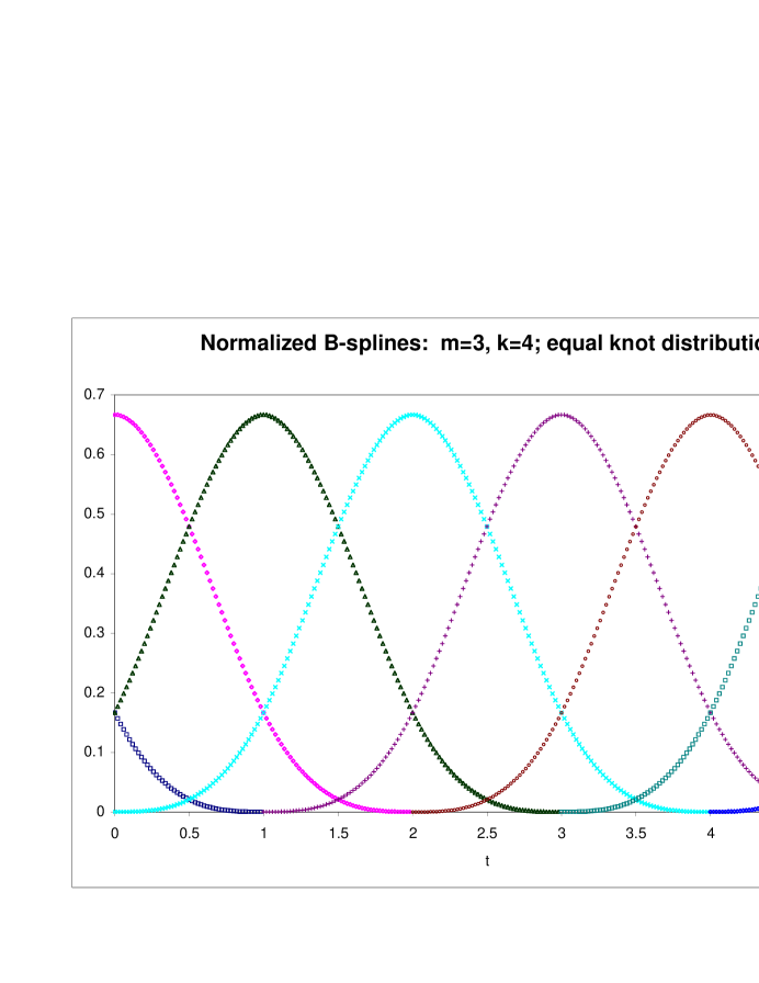
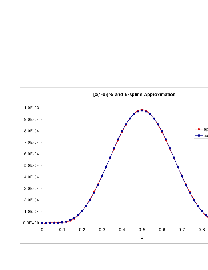
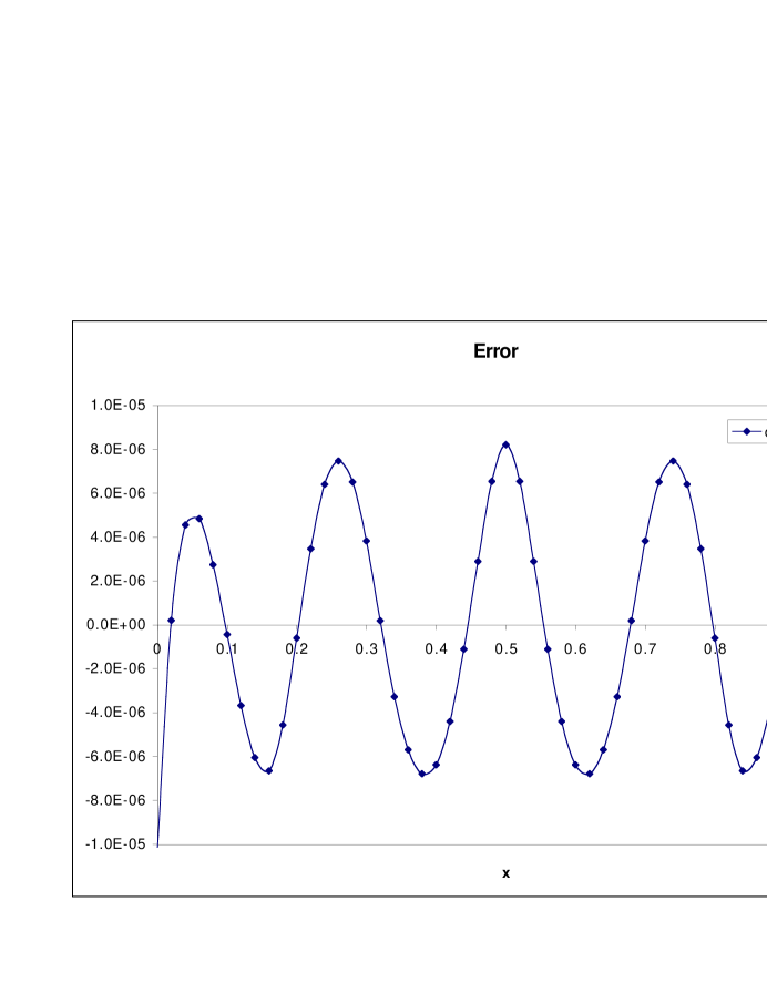
We want to know how well the B-splines are going to approximate functions that will come up in QCD. In the longitudinal direction, functions of the form $(x(1-x))^{d}$ where $d$ is positive, are common in light-front QCD. Figure 2 shows the function $(x(1-x))^{5}$ and the approximation built from B-splines with $m=3$ and $k=5$. The knot sequence is also uniform with separation $\frac{b-a}{k+1}$ where $a=0$ and $b=1$. Finally, figure 3 shows the difference between the exact function and the approximation using B-splines.

Figure 2: The function $(x(1-x))^{5}$ and the approximation using B-splines. The B-splines are order $m=3$ with $k=5$.

Figure 3: The difference between the function $(x(1-x))^{3}$ and the approximation using B-splines. The splines are order $m=3$ with $k=5$.

2 The One-Dimensional Harmonic Oscillator

To test the B-splines as a useful set of basis functions, we use them to solve the one-dimensional harmonic oscillator problem. The harmonic oscillator Hamiltonian is:

$$H=-\frac{\hbar^{2}}{2m}\frac{d^{2}}{dx^{2}}+\frac{1}{2}m\omega^{2}x^{2}.$$ (37)

If we write out the eigenvalue equation for a state $\phi$ that we approximate with B-splines we get:

$$H|\phi\rangle=E|\phi\rangle\rightarrow\sum_{i}a_{i}H|B_{i}\rangle=E\sum_{i}a_{i}|B_{i}\rangle.$$ (38)

Looking at a particular matrix element and dropping the explicit sum, we get:

$$\langle B_{j}|H|B_{i}\rangle a_{i}=\langle B_{j}|B_{i}\rangle Ea_{i},$$ (39)

where $\langle B_{j}|H|B_{i}\rangle$ is the Hamiltonian matrix ($H$) and $\langle B_{j}|B_{i}\rangle$ is the overlap matrix ($O$). This problem can be solved in its current form, as a generalized eigensystem problem

$$H{\bf x}=EO{\bf x},$$ (40)

or we can rewrite it as a simple eigensystem problem

$$O^{-1}H{\bf x}=E{\bf x}.$$ (41)

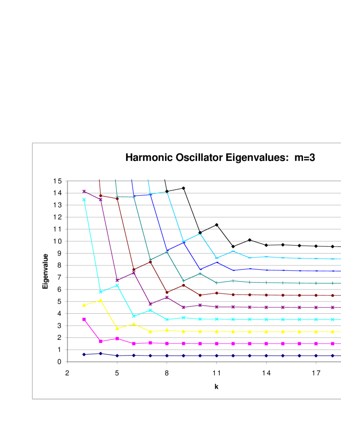
Since a B-spline of order $m$ has only $m-1$ continuous derivatives, it is necessary to use at least third-order B-splines. Although higher order B-splines may speed the convergence, they also add to the total number of states and matrix elements. For simplicity we use $m=3$ and only adjust $k$. Figure 4 shows the eigenvalues for the ten lowest states in units of $\hbar\omega$. Note the correct value of the energy is $E_{n}=(n+\frac{1}{2})\hbar\omega$, so the eigenvalues plotted approach the correct values. The total number of splines used is $m+k+1$, or for $m=3$, $k+4$. The knots are equally spaced over the range $[a,b]$ with $a=-5$ and $b=5$. $a$ and $b$ are determined by finding the smallest values that, when increased, do not change the eigenvalues.

Figure 4: Energy eigenvalues of the harmonic oscillator in units of $\hbar\omega$. The total number of states is $m+k+1$.

The harmonic oscillator can be solved analytically. The eigenfunctions are Hermite polynomials. We can see how well the B-splines approximate the solution by considering the overlap between the approximate and exact solutions. The overlap is defined as:

$$\frac{\int_{a}^{b}dx\phi(x)H(x)}{\int_{a}^{b}dxH^{2}(x)},$$ (42)

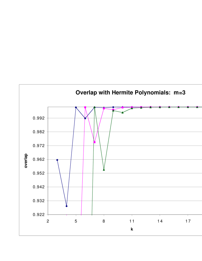
where $\phi(x)$ is the approximate solution built from B-splines and $H(x)$ is a Hermite polynomial. The overlap approaches $1$ as a better approximation is made. Figure 5 shows the overlap of the first three approximate eigenstates determined by B-spline approximation with the known solution to the harmonic oscillator problem, the Hermite polynomials.

Figure 5: Overlap of the harmonic oscillator eigenstates with the Hermite polynomials.

3 The Two-Dimensional Harmonic Oscillator

The two-dimensional harmonic oscillator is a non-trivial extension of the one-dimensional harmonic oscillator. The B-spline basis used for the two-dimensional problem is a product of the one-dimensional B-spline basis $B_{xy}=B_{x}\otimes B_{y}$ where $B_{x}$ and $B_{y}$ are one-dimensional B-spline basis. The energy for the two-dimensional case is simply the sum from each individual direction:

$$E_{(n_{x},n_{y})}=\frac{1}{2}(\omega_{x}+\omega_{y})+(n_{x}\omega_{x}+n_{y}\omega_{y}),$$ (43)

where $\hbar=1$.

Figure 6 shows the eigenvalues for the two-dimensional harmonic oscillator using third order B-splines in both the $x$ and $y$ directions. For convenience we use the same, equally spaced, knot distribution is used in both directions. The frequency in the $y$ direction is the same as in the $x$ direction which gives rise to the particular degeneracies shown.

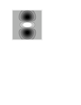
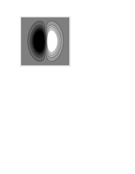
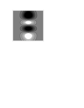
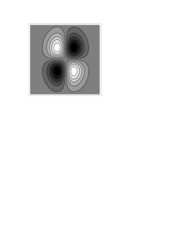
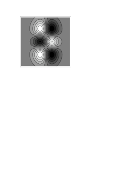
The approximation of the lowest seven states are plotted in figure 7. The ranges shown are limited to $-3<x,y<3$ because the harmonic oscillator states fall off exponentially. Note also the phase of the wave function is arbitrary (note the overall negative sign in the lowest state).

Figure 6: Eigenvalues for the two-dimensional harmonic oscillator, with $\omega_{x}=\omega_{y}=1$, and states labeled by $(n_{x},n_{y})$. There are k+m+1 states in each direction.

                 

                 

                 

Figure 7: The approximation of the seven of the lowest energy wave functions for the two-dimensional harmonic oscillator with $\omega_{y}=\omega_{x}=1$. The labels are : $(0,0)$, $(1,0)$, $(0,1)$, $(1,1)$, $(2,0)$, $(0,2)$ and $(2,1)$. There are k+m+1 states in each direction.

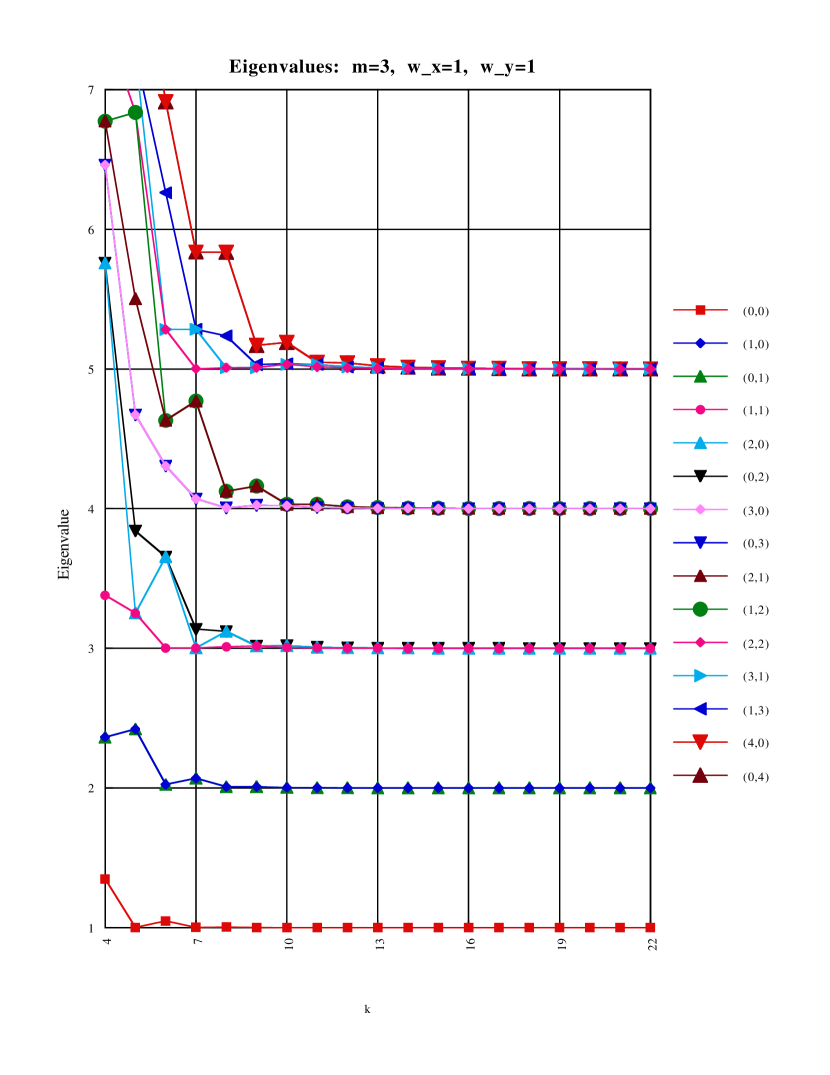
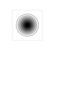
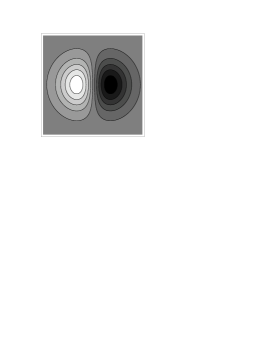
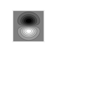
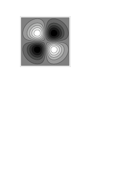
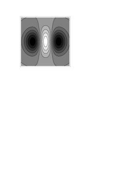
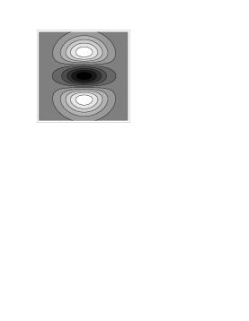
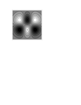
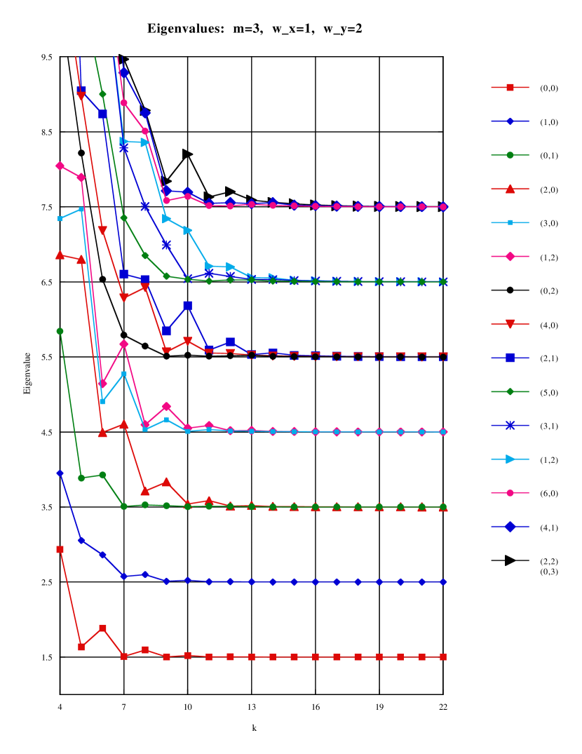
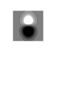
Figure 8 shows the eigenvalues for a two-dimensional harmonic oscillator without rotational symmetry using third order B-splines in both the $x$ and $y$ directions. For simplicity we use the same, equally spaced, knot distribution is used in both directions. The frequency in the $y$ direction is twice that in the $x$ direction which gives rise to the particular degeneracies shown. The approximation of the lowest seven states are plotted in figure 9. The ranges shown are limited to $-3<x,y<3$ because the harmonic oscillator states fall off exponentially. Note also the phase of the wave function is arbitrary (note the overall negative sign in the lowest state).

Figure 8: Eigenvalues for the two-dimensional anisotropic harmonic oscillator, with $\omega_{y}=2\omega_{x}=2$, and states labeled by $(n_{x},n_{y})$. There are k+m+1 states in each direction.

                 

                 

                 

Figure 9: The approximation of the seven of the lowest energy wave functions for the two-dimensional harmonic oscillator with $\omega_{y}=2\omega_{x}=2$. The labels are : $(0,0)$, $(1,0)$, $(2,0)$, $(0,1)$, $(3,0)$, $(1,1)$ and $(2,1)$. There are k+m+1 states in each direction.

Chapter 3 Matrix Elements of the Light-Front QCD Hamiltonian

In this chapter we quantize the Hamiltonian. We begin with the canonical light-front Hamiltonian [22] as a starting point. Splitting the Hamiltonian density into a free and interacting part, we have:

$${\cal H} = {\cal H}_{\mathrm{free}}+{\cal H}_{\mathrm{int}}$$ (1)

$${\cal H}_{\mathrm{int}} = {\cal H}_{qqg}+{\cal H}_{ggg}+{\cal H}_{qqgg}+{\cal H}_{qqqq}+{\cal H}_{gggg},$$ (2)

where

$${\cal H}_{qqg} = -g\left\{-2\psi^{\dagger}_{+}\left[\left(\frac{1}{\partial^{+}}\right)\left(\partial^{\bot}A^{\bot}\right)\right]\psi_{+}+\psi^{\dagger}_{+}\left(\sigma\cdot A^{\bot}\right)\right.$$ (3)

$$\hskip 56.9055pt\left.\left[\left(\frac{1}{\partial^{+}}\right)\left(\sigma\cdot\partial^{\bot}+m\right)\psi_{+}\right]\right.$$

$$\hskip 85.35826pt\left.+\psi^{\dagger}_{+}\left(\sigma\cdot\partial^{\bot}-m\right)\left[\left(\frac{1}{\partial^{+}}\right)\left(\sigma\cdot A_{\bot}\right)\psi_{+}\right]\right\},$$

$${\cal H}_{ggg} = -gf^{abc}\left\{A_{a}^{i}A_{b}^{j}\left(\partial^{i}A_{c}^{j}\right)+\left(\partial^{i}A_{a}^{i}\right)\left(\frac{1}{\partial^{+}}\right)\left[A_{b}^{j}\left(\partial^{+}A_{c}^{j}\right)\right]\right\},$$ (4)

$${\cal H}_{qqgg} = g^{2}\left\{\psi^{\dagger}_{+}\left(\sigma\cdot A^{\bot}\right)\left[\left(\frac{1}{i\partial^{+}}\right)\sigma\cdot A^{\bot}\psi_{+}\right]\right.$$ (5)

$$\hskip 56.9055pt\left.+2\left(\frac{1}{\partial^{+}}\right)\left[f^{abc}A_{b}^{i}\left(\partial^{+}A_{c}^{i}\right)\right]\left(\frac{1}{\partial^{+}}\right)\left(\psi^{\dagger}_{+}{\bf T}^{a}\psi_{+}\right)\right\},$$

$${\cal H}_{qqqq} = 2g^{2}\left\{\left(\frac{1}{\partial^{+}}\right)\left(\psi^{\dagger}_{+}{\bf T}_{a}\psi_{+}\right)\left(\frac{1}{\partial^{+}}\right)\left(\psi^{\dagger}_{+}{\bf T}_{a}\psi_{+}\right)\right\},$$ (6)

$${\cal H}_{gggg} = \frac{g^{2}}{4}f^{abc}f^{ade}\left\{A_{b}^{i}A_{c}^{j}A_{d}^{i}A_{e}^{j}\right.$$ (7)

$$\hskip 56.9055pt\left.+2\left(\frac{1}{\partial^{+}}\right)\left[A_{b}^{i}\left(\partial^{+}A_{c}^{i}\right)\right]\left(\frac{1}{\partial^{+}}\right)\left[A_{d}^{j}\left(\partial^{+}A_{e}^{j}\right)\right]\right\},$$

where the gluon and quark fields are defined in Appendix 10.

1 Conventions for the States

We order quark creation and annihilation operators, $b$ and $b^{\dagger}$ before antiquark creation and annihilation operators, $d$ and $d^{\dagger}$. If there is an initial state that contains a quark and an anti-quark, then the ordering will be $b^{\dagger}d^{\dagger}|0\rangle$. However, since the final state will be the complex conjugate of an initial state, the ordering in a final state will be $\langle 0|db$. Similarly, if a state contains two quarks, then we have: $|q_{1}q_{2}\rangle=b^{\dagger}_{1}b^{\dagger}_{2}|0\rangle$ and $|q_{1}q_{2}\rangle^{\dagger}=\langle q_{1}q_{2}|=\langle 0|b_{2}b_{1}$.

The results for the matrix elements of the Hamiltonian presented in Sections 3 and 4 are analogous to [37].

2 Quantization of the Hamiltonian

The full Hamiltonian can be written:

$$H=\int dx^{-}d^{2}x_{\bot}\left({\cal H}_{\mathrm{free}}+{\cal H}_{\mathrm{int}}\right).$$ (8)

We find:

$$H_{\mathrm{free}}=\int D_{1}\left\{\delta_{i,j}\frac{\left(p_{1}^{i}\right)^{2}}{p_{1}^{+}}a^{\dagger}_{1}a_{1}+\left(\frac{p^{2}_{\bot}+m^{2}}{p^{+}}\right)\left[b_{1}^{\dagger}b_{1}+d_{1}^{\dagger}d_{1}\right]\right\},$$ (9)

where $D_{1}$ is defined in Eq. (89)

The only parts of the interacting Hamiltonian we need to calculate for an ${\cal O}(g^{2})$ calculation are ${\cal H}_{qqg}$ and ${\cal H}_{qqqq}$. We label the transverse momentum of a particle $k_{a}^{(i)}$, where $a$ is the particle label and $(i)$ is the direction of the transverse momentum component. We define:

$$\tilde{k}_{3}^{s_{3}}=(s_{3})k_{3}^{(1)}+ik_{3}^{(2)},$$ (10)

and substitute the expressions for the gluon, quark and antiquark fields from 88, 114, and 115 into Eqs. (3) and (6) giving:

$$H_{q\bar{q}g} = 32\pi^{3}g\int D_{1}D_{3}D_{2}\sqrt{\frac{k_{1}^{+}\hskip 2.84544ptk_{2}^{+}}{2}}\langle c_{1}|{\bf T}^{c_{3}}|c_{2}\rangle\times$$ (11)

$$\left\{\delta^{3}(k_{1}+k_{2}-k_{3})\times\right.$$

$$\hskip 14.22636pt\left.\left[b^{\dagger}_{1}d^{\dagger}_{2}a_{3}\left(\delta_{s_{1},\bar{s}_{2}}\left\{-\frac{\tilde{k}_{3}^{s_{3}}}{k_{3}^{+}}+\delta_{\bar{s}_{2},s_{3}}\frac{\tilde{k}_{2}^{s_{3}}}{k_{2}^{+}}+\delta_{s_{2},s_{3}}\frac{\tilde{k}_{1}^{s_{3}}}{k_{1}^{+}}\right\}\right.\right.\right.$$

$$\hskip 113.81102pt\left.\left.\left.-ims_{2}\delta_{s_{1},s_{2}}\delta_{s_{2},s_{3}}\left\{\frac{1}{k_{2}^{+}}+\frac{1}{k_{1}^{+}}\right\}\right)\right.\right.$$

$$\hskip 56.9055pt\left.\left.-a^{\dagger}_{3}b_{2}d_{1}\left(\delta_{s_{1},\bar{s}_{2}}\left\{-\frac{\tilde{k}_{3}^{\ast s_{3}}}{k_{3}^{+}}+\delta_{\bar{s}_{2},s_{3}}\frac{\tilde{k}_{2}^{\ast s_{3}}}{k_{2}^{+}}+\delta_{s_{2},s_{3}}\frac{\tilde{k}_{1}^{\ast s_{3}}}{k_{1}^{+}}\right\}\right.\right.\right.$$

$$\hskip 142.26378pt\left.\left.\left.+ims_{2}\delta_{s_{1},s_{2}}\delta_{s_{2},s_{3}}\left\{\frac{1}{k_{2}^{+}}+\frac{1}{k_{1}^{+}}\right\}\right)\right]\right.$$

$$\left.+\delta^{3}(k_{1}-k_{2}-k_{3})\times\right.$$

$$\hskip 14.22636pt\left.\left[d^{\dagger}_{2}a^{\dagger}_{3}d_{1}\left(\delta_{s_{1},s_{2}}\left\{\frac{\tilde{k}_{3}^{\ast s_{3}}}{k_{3}^{+}}-\delta_{s_{2},s_{3}}\frac{\tilde{k}_{2}^{\ast s_{3}}}{k_{2}^{+}}-\delta_{s_{2},\bar{s}_{3}}\frac{\tilde{k}_{1}^{\ast s_{3}}}{k_{1}^{+}}\right\}\right.\right.\right.$$

$$\hskip 113.81102pt\left.\left.\left.-ims_{2}\delta_{s_{1},\bar{s}_{2}}\delta_{s_{2},\bar{s}_{3}}\left\{\frac{1}{k_{2}^{+}}-\frac{1}{k_{1}^{+}}\right\}\right)\right.\right.$$

$$\hskip 56.9055pt\left.\left.+b^{\dagger}_{1}b_{2}a_{3}\left(\delta_{s_{1},s_{2}}\left\{-\frac{\tilde{k}_{3}^{s_{3}}}{k_{3}^{+}}+\delta_{s_{2},s_{3}}\frac{\tilde{k}_{2}^{s_{3}}}{k_{2}^{+}}+\delta_{s_{2},\bar{s}_{3}}\frac{\tilde{k}_{1}^{s_{3}}}{k_{1}^{+}}\right\}\right.\right.\right.$$

$$\hskip 142.26378pt\left.\left.\left.-ims_{2}\delta_{s_{1},\bar{s}_{2}}\delta_{s_{2},\bar{s}_{3}}\left\{\frac{1}{k_{2}^{+}}-\frac{1}{k_{1}^{+}}\right\}\right)\right]\right.$$

$$\left.+\delta^{3}(k_{1}-k_{2}+k_{3})\times\right.$$

$$\hskip 14.22636pt\left.\left[b^{\dagger}_{1}a^{\dagger}_{3}b_{2}\left(\delta_{s_{1},s_{2}}\left\{-\frac{\tilde{k}_{3}^{\ast s_{3}}}{k_{3}^{+}}+\delta_{s_{2},\bar{s}_{3}}\frac{\tilde{k}_{2}^{\ast s_{3}}}{k_{2}^{+}}+\delta_{s_{2},s_{3}}\frac{\tilde{k}_{1}^{\ast s_{3}}}{k_{1}^{+}}\right\}\right.\right.\right.$$

$$\hskip 113.81102pt\left.\left.\left.+ims_{2}\delta_{s_{1},\bar{s}_{2}}\delta_{s_{2},s_{3}}\left\{\frac{1}{k_{2}^{+}}-\frac{1}{k_{1}^{+}}\right\}\right)\right.\right.$$

$$\hskip 56.9055pt\left.\left.+d^{\dagger}_{2}d_{1}a_{3}\left(\delta_{s_{1},s_{2}}\left\{\frac{\tilde{k}_{3}^{s_{3}}}{k_{3}^{+}}-\delta_{s_{2},\bar{s}_{3}}\frac{\tilde{k}_{2}^{s_{3}}}{k_{2}^{+}}-\delta_{s_{2},s_{3}}\frac{\tilde{k}_{1}^{s_{3}}}{k_{1}^{+}}\right\}\right.\right.\right.$$

$$\hskip 142.26378pt\left.\left.\left.+ims_{2}\delta_{s_{1},\bar{s}_{2}}\delta_{s_{2},s_{3}}\left\{\frac{1}{k_{2}^{+}}-\frac{1}{k_{1}^{+}}\right\}\right)\right]\right\}$$

and

$$H_{qqqq} = -32g^{2}\pi^{3}\int D_{1}D_{2}D_{3}D_{4}\langle c_{1}|{\bf T}_{a}|c_{2}\rangle\langle c_{3}|{\bf T}_{a}|c_{4}\rangle\sqrt{k_{1}^{+}k_{2}^{+}k_{3}^{+}k_{4}^{+}}\times$$ (12)

$$\left\{\delta^{3}(k_{1}-k_{2}+k_{3}-k_{4})\frac{\delta_{s_{1},s_{2}}\delta_{s_{3},s_{4}}}{(k_{1}^{+}-k_{2}^{+})^{2}}\left[b^{\dagger}_{1}b^{\dagger}_{3}b_{2}b_{4}+d^{\dagger}_{2}d^{\dagger}_{4}d_{1}d_{3}\right]\right.$$

$$\left.+\delta^{3}(k_{1}+k_{2}+k_{3}-k_{4})\frac{\delta_{s_{1},-s_{2}}\delta_{s_{3},s_{4}}}{(k_{1}^{+}+k_{2}^{+})^{2}}\left[b^{\dagger}_{1}b^{\dagger}_{3}d^{\dagger}_{2}b_{4}-d^{\dagger}_{4}b_{2}d_{1}d_{3}\right]\right.$$

$$\left.-\delta^{3}(k_{1}-k_{2}+k_{3}+k_{4})\frac{\delta_{s_{1},s_{2}}\delta_{s_{3},-s_{4}}}{(k_{1}^{+}-k_{2}^{+})^{2}}\left[b^{\dagger}_{1}b^{\dagger}_{3}d^{\dagger}_{4}b_{2}-d^{\dagger}_{2}b_{4}d_{1}d_{3}\right]\right.$$

$$\left.+\delta^{3}(k_{1}+k_{2}-k_{3}+k_{4})\frac{\delta_{s_{1},-s_{2}}\delta_{s_{3},s_{4}}}{(k_{1}^{+}+k_{2}^{+})^{2}}\left[b^{\dagger}_{1}d^{\dagger}_{2}d^{\dagger}_{4}d_{3}-b^{\dagger}_{3}b_{2}b_{4}d_{1}\right]\right.$$

$$\left.-\delta^{3}(k_{1}-k_{2}-k_{3}+k_{4})\frac{\delta_{s_{1},s_{2}}\delta_{s_{3},s_{4}}}{(k_{1}^{+}-k_{2}^{+})^{2}}\left[b^{\dagger}_{1}d^{\dagger}_{4}b_{2}d_{3}+b^{\dagger}_{3}d^{\dagger}_{2}b_{4}d_{1}\right]\right.$$

$$\left.+\delta^{3}(k_{1}+k_{2}-k_{3}-k_{4})\frac{\delta_{s_{1},-s_{2}}\delta_{s_{3},-s_{4}}}{(k_{1}^{+}+k_{2}^{+})^{2}}\left[b^{\dagger}_{1}d^{\dagger}_{2}b_{4}d_{3}+b^{\dagger}_{3}d^{\dagger}_{4}b_{2}d_{1}\right]\right.$$

$$\left.+\delta_{3}(k_{1}-k_{2}-k_{3}-k_{4})\frac{\delta_{s_{1},s_{2}}\delta_{s_{3},-s_{4}}}{(k_{1}^{+}-k_{2}^{+})^{2}}\left[b^{\dagger}_{1}b_{2}b_{4}d_{3}-b^{\dagger}_{3}d^{\dagger}_{2}d^{\dagger}_{4}d_{1}\right]\right\}.$$

3 $q\bar{q}g$ Matrix Elements

We need to find the matrix elements of all $q\bar{q}g$ vertices.

1 $\langle q_{a}\bar{q}_{b}|H|g_{c}\rangle$

This gives us:

$$\langle q_{a}\bar{q}_{b}|H|g_{c}\rangle=$$ (13)

$$\hskip 56.9055pt16\pi^{3}g\sqrt{2k_{a}^{+}k_{b}^{+}}\langle c_{a}|{\bf T}^{c_{c}}|c_{b}\rangle\delta^{3}(k_{a}+k_{b}-k_{c})\times$$

$$\hskip 113.81102pt\left(\delta_{s_{a},\bar{s}_{b}}\left\{-\frac{\tilde{k}_{c}^{s_{c}}}{k_{c}^{+}}+\delta_{\bar{s}_{b},s_{c}}\frac{\tilde{k}_{b}^{s_{c}}}{k_{b}^{+}}+\delta_{s_{b},s_{c}}\frac{\tilde{k}_{a}^{s_{c}}}{k_{a}^{+}}\right\}\right.$$

$$\hskip 170.71652pt\left.-ims_{b}\delta_{s_{a},s_{b}}\delta_{s_{b},s_{c}}\left\{\frac{1}{k_{b}^{+}}+\frac{1}{k_{a}^{+}}\right\}\right).$$

2 $\langle g_{c}|H|q_{a}\bar{q}_{b}\rangle$

$$\langle g_{c}|H|q_{a}\bar{q}_{b}\rangle=$$

$$\hskip 56.9055pt16\pi^{3}g\sqrt{2k_{a}^{+}k_{b}^{+}}\langle c_{b}|{\bf T}^{c_{c}}|c_{a}\rangle\delta^{3}(k_{a}+k_{b}-k_{c})\times$$

$$\hskip 113.81102pt\left(\delta_{s_{b},\bar{s}_{a}}\left\{-\frac{\tilde{k}_{c}^{\ast s_{c}}}{k_{c}^{+}}+\delta_{\bar{s}_{a},s_{c}}\frac{\tilde{k}_{a}^{\ast s_{c}}}{k_{a}^{+}}+\delta_{s_{a},s_{c}}\frac{\tilde{k}_{b}^{\ast s_{c}}}{k_{b}^{+}}\right\}\right.$$

$$\hskip 170.71652pt\left.+ims_{a}\delta_{s_{b},s_{a}}\delta_{s_{a},s_{c}}\left\{\frac{1}{k_{a}^{+}}+\frac{1}{k_{b}^{+}}\right\}\right).$$ (14)

3 $\langle\bar{q}_{b}g_{c}|H|\bar{q}_{a}\rangle$

$$\langle\bar{q}_{b}g_{c}|H|\bar{q}_{a}\rangle=$$

$$\hskip 56.9055pt16\pi^{3}g\sqrt{2k_{a}^{+}k_{b}^{+}}\langle c_{a}|{\bf T}^{c_{c}}|c_{b}\rangle\delta^{3}(k_{a}-k_{b}-k_{c})\times$$

$$\hskip 113.81102pt\left(\delta_{s_{a},s_{b}}\left\{\frac{\tilde{k}_{c}^{\ast s_{c}}}{k_{c}^{+}}-\delta_{s_{b},s_{c}}\frac{\tilde{k}_{b}^{\ast s_{c}}}{k_{b}^{+}}-\delta_{s_{b},\bar{s}_{c}}\frac{\tilde{k}_{a}^{\ast s_{c}}}{k_{a}^{+}}\right\}\right.$$

$$\hskip 170.71652pt\left.-ims_{b}\delta_{s_{a},\bar{s}_{b}}\delta_{s_{b},\bar{s}_{c}}\left\{\frac{1}{k_{b}^{+}}-\frac{1}{k_{a}^{+}}\right\}\right).$$ (15)

4 $\langle q_{a}|H|q_{b}g_{c}\rangle$

$$\langle q_{a}|H|q_{b}g_{c}\rangle=$$

$$\hskip 56.9055pt16\pi^{3}g\sqrt{2k_{a}^{+}k_{b}^{+}}\langle c_{a}|{\bf T}^{c_{c}}|c_{b}\rangle\delta^{3}(k_{a}-k_{b}-k_{c})\times$$

$$\hskip 113.81102pt\left(\delta_{s_{a},s_{b}}\left\{-\frac{\tilde{k}_{c}^{s_{c}}}{k_{c}^{+}}+\delta_{s_{b},s_{c}}\frac{\tilde{k}_{b}^{s_{c}}}{k_{b}^{+}}+\delta_{s_{b},\bar{s}_{c}}\frac{\tilde{k}_{a}^{s_{c}}}{k_{a}^{+}}\right\}\right.$$

$$\hskip 170.71652pt\left.-ims_{b}\delta_{s_{a},\bar{s}_{b}}\delta_{s_{b},\bar{s}_{c}}\left\{\frac{1}{k_{b}^{+}}-\frac{1}{k_{a}^{+}}\right\}\right).$$ (16)

5 $\langle q_{a}g_{c}|H|q_{b}\rangle$

$$\langle q_{a}g_{c}|H|q_{b}\rangle=$$

$$\hskip 56.9055pt16\pi^{3}g\sqrt{2k_{a}^{+}k_{b}^{+}}\langle c_{a}|{\bf T}^{c_{c}}|c_{b}\rangle\delta^{3}(k_{a}-k_{b}+k_{c})\times$$

$$\hskip 113.81102pt\left(\delta_{s_{a},s_{b}}\left\{-\frac{\tilde{k}_{c}^{\ast s_{c}}}{k_{c}^{+}}+\delta_{s_{b},\bar{s}_{c}}\frac{\tilde{k}_{b}^{\ast s_{c}}}{k_{b}^{+}}+\delta_{s_{b},s_{c}}\frac{\tilde{k}_{a}^{\ast s_{c}}}{k_{a}^{+}}\right\}\right.$$

$$\hskip 170.71652pt\left.+ims_{b}\delta_{s_{a},\bar{s}_{b}}\delta_{s_{b},s_{c}}\left\{\frac{1}{k_{b}^{+}}-\frac{1}{k_{a}^{+}}\right\}\right).$$ (17)

6 $\langle\bar{q}_{a}|H|\bar{q}_{b}g_{c}\rangle$

$$\langle\bar{q}_{a}|H|\bar{q}_{b}g_{c}\rangle=$$ (18)

$$\hskip 56.9055pt16\pi^{3}g\sqrt{2k_{a}^{+}k_{b}^{+}}\langle c_{b}|{\bf T}^{c_{c}}|c_{a}\rangle\delta^{3}(k_{b}-k_{a}+k_{c})\times$$

$$\hskip 113.81102pt\left(\delta_{s_{b},s_{a}}\left\{\frac{\tilde{k}_{c}^{s_{c}}}{k_{c}^{+}}-\delta_{s_{a},\bar{s}_{c}}\frac{\tilde{k}_{a}^{s_{c}}}{k_{a}^{+}}-\delta_{s_{a},s_{c}}\frac{\tilde{k}_{b}^{s_{c}}}{k_{b}^{+}}\right\}\right.$$

$$\hskip 170.71652pt\left.+ims_{a}\delta_{s_{b},\bar{s}_{a}}\delta_{s_{a},s_{c}}\left\{\frac{1}{k_{a}^{+}}-\frac{1}{k_{b}^{+}}\right\}\right).$$

4 $q\bar{q}q\bar{q}$ Matrix Elements

To calculate a $q\bar{q}$ state to second order, it is only necessary to calculate the instantaneous exchange matrix element.

There are two different terms for the instantaneous exchange which give us:

$$\langle q_{a}\bar{q}_{b}|H|q_{c}\bar{q}_{d}\rangle_{\mathrm{IN}} = -32g^{2}\pi^{3}\int D_{1}D_{2}D_{3}D_{4}\langle c_{1}|{\bf T}_{a}|c_{2}\rangle\langle c_{3}|{\bf T}_{a}|c_{4}\rangle\sqrt{k_{1}^{+}k_{2}^{+}k_{3}^{+}k_{4}^{+}}\times$$ (19)

$$\delta^{3}(k_{1}-k_{2}-k_{3}+k_{4})\frac{\delta_{s_{1},s_{2}}\delta_{s_{3},s_{4}}}{(k_{1}^{+}-k_{2}^{+})^{2}}\left[\delta_{a,1}\delta_{b,4}\delta_{c,2}\delta_{d,3}+\delta_{a,3}\delta_{b,2}\delta_{c,4}\delta_{d,1}\right].$$

The two different sets of delta functions give identical contributions when we use the momentum conserving delta function. Thus, we get:

$$\langle q_{a}\bar{q}_{b}|H|q_{c}\bar{q}_{d}\rangle = -64g^{2}\pi^{3}\langle c_{d}|{\bf T}_{f}|c_{b}\rangle\langle c_{a}|{\bf T}_{f}|c_{c}\rangle\sqrt{k_{a}^{+}k_{b}^{+}k_{c}^{+}k_{d}^{+}}\times$$ (20)

$$\hskip 56.9055pt\delta^{3}(k_{a}-k_{c}-k_{d}+k_{b})\frac{\delta_{s_{a},s_{c}}\delta_{s_{b},s_{d}}}{(k_{a}^{+}-k_{c}^{+})^{2}}.$$

Chapter 4 Matrix Elements of the Renormalized Hamiltonian

We now determine the matrix elements of our renormalized Hamiltonian in a plane-wave basis. Section 6 shows which matrix elements are needed to calculate the mass-squared operator to second order. These matrix elements are calculated in Sections 1 through 3.

We find matrix elements of the IMO which is very closely related to the Hamiltonian matrix elements we have already calculated. Specifically, in the center-of-momentum frame

$${\cal M}^{2}={\cal P}^{+}{\cal H},$$ (1)

where ${\cal P}^{+}$ is the total light-front longitudinal momentum.

1 Cutoff Dependent, Non-Canonical Contributions

The non-canonical contributions to the mass matrix are contained in
$\langle{q_{3}\bar{q}_{4}}|V_{\mathrm{C\hskip 0.56905ptD}}^{(2)}(\Lambda)|{q_{1}\bar{q}_{2}}\rangle$, or more explicitly in $\left<F\right|\delta V^{(2)}\left|I\right>$ [Eq. (44)]. For a second order calculation, we can write:

$$\left<F\right|\delta V^{(2)}\left|I\right>=\frac{1}{2}\sum_{K}\langle{q_{3}\bar{q}_{4}}|V^{(1)}|{K}\rangle\langle{K}|V^{(1)}|{q_{1}\bar{q}_{2}}\rangle T_{2}^{(\Lambda,\Lambda^{\prime})}(F,K,I),$$ (2)

where the sum is over a complete set of (intermediate) states and $V^{(1)}$ is the first-order canonical Hamiltonian. The only term in $V^{(1)}$ we need contains a $q\bar{q}g$ vertex so $|K\rangle$ can only be a $q\bar{q}g$ state, and the interaction is either a gluon exchange or a quark self-energy.

In this section, we make the following momentum definitions for various momenta in the self-energy and exchange diagrams:

$$k_{1} = (x{\cal P}^{+},x\vec{{\cal P}}+\vec{q_{\bot}}),\hskip 14.22636ptk_{2}=([1-x]{\cal P}^{+},[1-x]\vec{{\cal P}}-\vec{q_{\bot}}),$$

$$k_{3} = (y{\cal P}^{+},y\vec{{\cal P}}+\vec{p_{\bot}}),\hskip 14.22636ptk_{4}=([1-y]{\cal P}^{+},[1-y]\vec{{\cal P}}-\vec{p_{\bot}}),$$

$$k_{5} = (zk_{1}^{+},z\vec{k}_{1}+\vec{r_{\bot}}),\hskip 14.22636ptk_{7}=([1-z]k_{1}^{+},[1-z]\vec{k}_{1}-\vec{r_{\bot}}),$$ (3)

where $k_{1}$ and $k_{3}$ are the momentum of the incoming and outgoing quark and anti-quark, respectively. $k_{5}$ is the momentum of the internal quark. Using these definitions, we find for the free mass squared of the states:

$$M_{f}^{2}|F\rangle = M_{f}^{2}|q_{3}\bar{q}_{4}\rangle=\frac{\vec{p}_{\perp}^{\hskip 1.42271pt2}+m^{2}}{y(1-y)},$$ (4)

$$M_{f}^{2}|I\rangle = M_{f}^{2}|q_{1}\bar{q}_{2}\rangle=\frac{\vec{q}_{\perp}^{\hskip 1.42271pt2}+m^{2}}{x(1-x)},$$ (5)

$$M_{f}^{2}|K\rangle = M_{f}^{2}|q_{5}\bar{q}_{6}g_{7}\rangle$$ (6)

$$= \frac{m^{2}(1-z)(1-x+xz)+z(1-z)\vec{q}_{\perp}^{\hskip 1.42271pt2}+(1-x)\vec{r}_{\perp}^{\hskip 1.42271pt2}}{x(1-x)z(1-z)}.$$

1 Self-Energy

The quark self-energy contribution to $\left<F\right|\delta V^{(2)}\left|I\right>$ is:

$$\frac{1}{2}\int D_{5}D_{6}D_{7}\langle q_{3}\bar{q}_{4}|V^{(1)}_{qg\rightarrow q}|q_{5}\bar{q}_{6}g_{7}\rangle\langle q_{5}\bar{q}_{6}g_{7}|V^{(1)}_{q\rightarrow qg}|q_{1}\bar{q}_{2}\rangle T_{2}(F,K_{\mathrm{SE}},I),$$ (7)

where the subscript on $V^{(1)}$ indicates which of the vertices calculated in Section 3 are used. For the quark self-energy we will need the matrix elements given in Eqs. (4) and (5). However, these are not the complete matrix elements, since there is a spectator quark. We use:

$$\langle q_{5}\bar{q}_{6}g_{7}|V^{(1)}|\bar{q}_{2}q_{1}\rangle=$$

$$\hskip 28.45274pt16\pi^{3}{\cal P}^{+}\int D_{1}D_{2}D_{7}D_{5}D_{6}\sqrt{2k_{5}^{+}k_{1}^{+}}{\bf T}^{7}_{5,1}\delta^{3}(k_{5}-k_{1}+k_{7})\delta_{2,6}\times$$

$$\hskip 85.35826pt\left(\delta_{s_{5},s_{1}}\left\{-\frac{\tilde{k}_{7}^{\ast s_{7}}}{k_{7}^{+}}+\delta_{s_{1},\bar{s}_{7}}\frac{\tilde{k}_{1}^{\ast s_{7}}}{k_{1}^{+}}+\delta_{s_{1},s_{7}}\frac{\tilde{k}_{5}^{\ast s_{7}}}{k_{5}^{+}}\right\}\right.$$

$$\hskip 184.9429pt\left.+ims_{1}\delta_{s_{5},\bar{s}_{1}}\delta_{s_{1},s_{7}}\left\{\frac{1}{k_{1}^{+}}-\frac{1}{k_{5}^{+}}\right\}\right),$$ (8)

and

$$\langle\bar{q}_{4}q_{3}|V^{(1)}|q_{5}\bar{q}_{6}g_{7}\rangle=$$

$$\hskip 28.45274pt16\pi^{3}{\cal P}^{+}\int D_{3}D_{4}D_{7}D_{5}D_{6}\sqrt{2k_{3}^{+}k_{5}^{+}}{\bf T}^{7}_{3,5}\delta^{3}(k_{3}-k_{5}-k_{7})\delta_{4,6}\times$$

$$\hskip 85.35826pt\left(\delta_{s_{3},s_{5}}\left\{-\frac{\tilde{k}_{7}^{s_{7}}}{k_{7}^{+}}+\delta_{s_{5},s_{7}}\frac{\tilde{k}_{5}^{s_{7}}}{k_{5}^{+}}+\delta_{s_{5},\bar{s}_{7}}\frac{\tilde{k}_{3}^{s_{7}}}{k_{3}^{+}}\right\}\right.$$

$$\hskip 184.9429pt\left.-ims_{5}\delta_{s_{3},\bar{s}_{5}}\delta_{s_{5},\bar{s}_{7}}\left\{\frac{1}{k_{5}^{+}}-\frac{1}{k_{3}^{+}}\right\}\right).$$ (9)

Thus the contribution from the quark self-energy diagram can be written:

$$(16\pi^{3}{\cal P}^{+})^{2}\delta_{2,4}\int D_{5}D_{7}k_{5}^{+}\sqrt{k_{1}^{+}k_{3}^{+}}{\bf T}^{7}_{3,5}{\bf T}^{7}_{5,1}\delta^{3}(k_{3}-k_{5}-k_{7})\delta^{3}(k_{5}-k_{1}+k_{7})$$

$$\hskip 56.9055pt\times\left(\delta_{s_{5},s_{1}}\left\{-\frac{\tilde{k}_{7}^{\ast s_{7}}}{k_{7}^{+}}+\delta_{s_{1},\bar{s}_{7}}\frac{\tilde{k}_{1}^{\ast s_{7}}}{k_{1}^{+}}+\delta_{s_{1},s_{7}}\frac{\tilde{k}_{5}^{\ast s_{7}}}{k_{5}^{+}}\right\}\right.$$

$$\hskip 170.71652pt\left.+ims_{1}\delta_{s_{5},\bar{s}_{1}}\delta_{s_{1},s_{7}}\left\{\frac{1}{k_{1}^{+}}-\frac{1}{k_{5}^{+}}\right\}\right)$$

$$\hskip 85.35826pt\times\left(\delta_{s_{3},s_{5}}\left\{-\frac{\tilde{k}_{7}^{s_{7}}}{k_{7}^{+}}+\delta_{s_{3},s_{7}}\frac{\tilde{k}_{5}^{s_{7}}}{k_{5}^{+}}+\delta_{s_{3},\bar{s}_{7}}\frac{\tilde{k}_{3}^{s_{7}}}{k_{3}^{+}}\right\}\right.$$

$$\hskip 199.16928pt\left.+ims_{3}\delta_{s_{3},\bar{s}_{5}}\delta_{s_{5},\bar{s}_{7}}\left\{\frac{1}{k_{5}^{+}}-\frac{1}{k_{3}^{+}}\right\}\right)$$

$$\hskip 113.81102pt\times T_{2}^{(\Lambda,\Lambda^{\prime})}(F,K,I).$$ (10)

After integrating over everything but the momentum of the internal quark, and completing all sums, this becomes:

$$\frac{\delta_{1,3}\delta_{2,4}}{12\pi^{3}}\int\frac{dzd^{2}\vec{r}_{\bot}}{(1-z)^{3}z^{2}}\frac{m^{2}(z-1)^{4}+\vec{r}_{\bot}^{\hskip 2.84544pt2}(1+z^{2})}{x^{2}}\hskip 1.42271ptT_{2}^{(\Lambda,\Lambda^{\prime})}(F,K,I).$$ (11)

Recall that $z=k^{+}_{5}/k^{+}_{1}$. For the self-energy, the final and initial states have the same energy giving:

$$\Delta_{FK}=-\Delta_{KI}=-\frac{\vec{r}^{\hskip 1.42271pt2}+m^{2}(1-z)^{2}}{xz(1-z)},$$ (12)

and

$$T_{2}^{(\Lambda,\Lambda^{\prime})}(F,K,I)=-\frac{2}{\Delta_{KI}}\left(e^{-2\Lambda^{\prime-4}\Delta_{KI}^{2}}-e^{-2\Lambda^{-4}\Delta_{KI}^{2}}\right).$$ (13)

Using the definitions:

$$u = \frac{m^{2}(1-z)^{2}+r^{2}}{xz(1-z)},\hskip 28.45274pt\beta=\frac{m^{2}(1-z)}{xz},$$

$$\gamma(a,b) = \sqrt{2}\frac{m^{2}}{\Lambda^{2}}\frac{(1-b)}{ab},\hskip 28.45274pt\gamma^{\prime}(a,b)=\sqrt{2}\frac{m^{2}}{\Lambda^{\prime 2}}\frac{(1-b)}{ab},$$

and changing variables from $r$ to $u$ and integrating over $u$ gives:

$$-\Lambda^{\prime 2}\frac{\delta_{1,3}\delta_{2,4}}{24\pi^{2}}\left[\int\frac{z\hskip 2.84544ptdz}{1-z}\left\{\frac{1+z^{2}}{z}\sqrt{2\pi}\left[1-\mathrm{erf}\left(\gamma^{\prime}(x,z)\right)\right]\right.\right.$$

$$\hskip 113.81102pt\left.\left.-2\sqrt{2}\gamma^{\prime}(x,z)\mathrm{Ei}\left(1,\gamma^{\prime 2}(x,z)\right)\right\}\right]-\left[\Lambda^{\prime}\rightarrow\Lambda\right]$$ (14)

for the contribution to $\left<F\right|\delta V^{(2)}\left|I\right>$ from the quark self-energy, where ‘erf’ is the error function and ‘Ei’ is the exponential integral. The anti-quark self-energy contribution to $\left<F\right|\delta V^{(2)}\left|I\right>$ is:

$$\frac{1}{2}\int D_{5}D_{6}D_{7}\langle q_{3}\bar{q}_{4}|V^{(1)}_{\bar{q}g\rightarrow\bar{q}}|q_{5}\bar{q}_{6}g_{7}\rangle\langle q_{5}\bar{q}_{6}g_{7}|V^{(1)}_{\bar{q}\rightarrow\bar{q}g}|q_{1}\bar{q}_{2}\rangle T_{2}(F,K_{\mathrm{SE}},I),$$ (15)

where the subscript on $V^{(1)}$ indicates which of the vertices calculated in Section 3 is used.

The contribution from the anti-quark self-energy is the same as that from the quark self-energy with $x\rightarrow 1-x$. So we find the total contribution to $\delta V$ from the self-energy diagrams is:

$$\frac{\delta_{1,3}\delta_{2,4}}{24\pi^{2}}\Lambda^{\prime 2}\left[\int\frac{z\hskip 2.84544ptdz}{1-z}\left\{\frac{1+z^{2}}{z}\sqrt{2\pi}\left[\mathrm{erf}\left(\gamma^{\prime}(x,z)\right)+\mathrm{erf}\left(\gamma^{\prime}(1-x,z)\right)-2\right]\right.\right.$$

$$\hskip 85.35826pt\left.\left.+\sqrt{8}\left[\gamma^{\prime}(x,z)\mathrm{Ei}\left(1,\gamma^{\prime 2}(x,z)\right)\right.\right.\right.$$

$$\hskip 142.26378pt\left.\left.\left.+\gamma^{\prime}(1-x,z)\mathrm{Ei}\left(1,\gamma^{\prime 2}(1-x,z)\right)\right]\right\}\right]$$

$$\hskip 56.9055pt-\left[\Lambda^{\prime}\rightarrow\Lambda\right].$$ (16)

To find $\langle q_{3}\bar{q}_{4}|V^{(2)}_{\mathrm{SE}}(\Lambda)|q_{1}\bar{q}_{2}\rangle$ we have to keep only the $\Lambda$ terms and remove the cutoff independent part. We remove the cutoff independent part by expanding our answer in a generalized series of powers and logs of $\frac{m}{\Lambda}$ and remove the part proportional to $m^{2}$.

Keeping only the terms that contain $\Lambda$ gives us:

$$-\frac{\delta_{1,3}\delta_{2,4}}{24\pi^{2}}\Lambda^{2}\left[\int\frac{z\hskip 2.84544ptdz}{1-z}\left\{\frac{1+z^{2}}{z}\sqrt{2\pi}\left[\mathrm{erf}\left(\gamma(x,z)\right)+\mathrm{erf}\left(\gamma(1-x,z)\right)-2\right]\right.\right.$$

$$\hskip 28.45274pt\left.\left.+\sqrt{8}\left[\gamma(x,z)\mathrm{Ei}\left(1,\gamma^{2}(x,z)\right)+\gamma(1-x,z)\mathrm{Ei}\left(1,\gamma^{2}(1-x,z)\right)\right]\right\}\right].$$ (17)

Finally, we have to remove the terms that are independent of the cutoff, since they can not be determined by calculating $\delta V$. The only part of this expression that contains terms proportional to $m^{2}$ are the error functions. We find the cutoff-independent part of this expression to be:

$$-4\frac{\delta_{1,3}\delta_{2,4}}{24\pi^{2}}m^{2}\int dz\frac{1+z^{2}}{zx(1-x)}.$$ (18)

This term is divergent, however the entire term will be cancelled when calculating the cutoff independent part of the reduced interaction (Sec. 3). Thus the complete expression for $\langle q_{3}\bar{q}_{4}|V^{(2)}_{\mathrm{SE}}(\Lambda)|q_{1}\bar{q}_{2}\rangle$ is:

$$\langle q_{3}\bar{q}_{4}|V^{(2)}_{\mathrm{SE}}(\Lambda)|q_{1}\bar{q}_{2}\rangle=-\Lambda^{2}\frac{\delta_{1,3}\delta_{2,4}}{24\pi^{2}}\times$$

$$\hskip 28.45274pt\left[\int\frac{z\hskip 2.84544ptdz}{1-z}\left\{\frac{1+z^{2}}{z}\sqrt{2\pi}\left[\mathrm{erf}\left(\gamma(x,z)\right)+\mathrm{erf}\left(\gamma(1-x,z)\right)-2\right]\right.\right.$$

$$\hskip 85.35826pt\left.\left.+\sqrt{8}\left(\gamma(x,z)\mathrm{Ei}\left[1,\gamma^{2}(x,z)\right]\right.\right.\right.$$

$$\hskip 170.71652pt\left.\left.\left.+\gamma(1-x,z)\mathrm{Ei}\left[1,\gamma^{2}(1-x,z)\right]\right)\right\}\right.$$

$$\hskip 142.26378pt\left.-4m^{2}\int dz\frac{1+z^{2}}{zx(1-x)}\right].$$ (19)

2 Exchange

The first exchange diagram contributes to $\left<F\right|\delta V^{(2)}\left|I\right>$:

$$\frac{1}{2}\int D_{5}D_{6}D_{7}\langle q_{3}\bar{q}_{4}|V^{(1)}_{\bar{q}g\rightarrow\bar{q}}|q_{5}\bar{q}_{6}g_{7}\rangle\langle q_{5}\bar{q}_{6}g_{7}|V^{(1)}_{q\rightarrow qg}|q_{1}\bar{q}_{2}\rangle T_{2}(F,K_{\mathrm{EX}},I),$$ (20)

where the subscript on $V^{(1)}$ indicates which of the vertices calculated in Section 3 is used. For this exchange diagram, we need to use the matrix elements derived from Eqs. (5) and (18):

$$\langle q_{5}\bar{q}_{6}g_{7}|V^{(1)}|q_{1}\bar{q}_{2}\rangle = 16\pi^{3}{\cal P}^{+}\sqrt{2k_{5}^{+}k_{1}^{+}}\langle c_{5}|{\bf T}^{c_{7}}|c_{1}\rangle\delta_{2,6}\delta^{3}(k_{5}-k_{1}+k_{7})\times$$ (21)

$$\left(\delta_{s_{5},s_{1}}\left\{-\frac{\tilde{k}_{7}^{\ast s_{7}}}{k_{7}^{+}}+\delta_{s_{1},\bar{s}_{7}}\frac{\tilde{k}_{1}^{\ast s_{7}}}{k_{1}^{+}}+\delta_{s_{1},s_{7}}\frac{\tilde{k}_{5}^{\ast s_{7}}}{k_{5}^{+}}\right\}\right.$$

$$\hskip 85.35826pt\left.+ims_{1}\delta_{s_{5},\bar{s}_{1}}\delta_{s_{1},s_{7}}\left\{\frac{1}{k_{1}^{+}}-\frac{1}{k_{5}^{+}}\right\}\right),$$

$$\langle q_{3}\bar{q}_{4}|V^{(1)}|q_{1}\bar{q}_{2}g_{7}\rangle = 16\pi^{3}{\cal P}^{+}\sqrt{2k_{4}^{+}k_{6}^{+}}\langle c_{6}|{\bf T}^{c_{7}}|c_{4}\rangle\delta_{3,5}\delta^{3}(k_{6}-k_{4}+k_{7})\times$$ (22)

$$\left(\delta_{s_{6},s_{4}}\left\{\frac{\tilde{k}_{7}^{s_{7}}}{k_{7}^{+}}-\delta_{s_{4},\bar{s}_{7}}\frac{\tilde{k}_{4}^{s_{7}}}{k_{4}^{+}}-\delta_{s_{4},s_{7}}\frac{\tilde{k}_{6}^{s_{7}}}{k_{6}^{+}}\right\}\right.$$

$$\hskip 85.35826pt\left.+ims_{4}\delta_{s_{6},\bar{s}_{4}}\delta_{s_{4},s_{7}}\left\{\frac{1}{k_{4}^{+}}-\frac{1}{k_{6}^{+}}\right\}\right).$$

The total contribution from this exchange diagram is:

$$- (16\pi^{3}{\cal P}^{+})^{2}\int D_{7}\sqrt{k_{1}^{+}k_{2}^{+}k_{3}^{+}k_{4}^{+}}{\bf T}^{7}_{5,1}{\bf T}^{7}_{6,4}\delta^{3}(k_{2}-k_{4}+k_{7})\delta^{3}(k_{3}-k_{1}+k_{7})$$ (23)

$$\hskip 56.9055pt\times\left(\delta_{s_{3},s_{1}}\left\{-\frac{\tilde{k}_{7}^{\ast s_{7}}}{k_{7}^{+}}+\delta_{s_{1},\bar{s}_{7}}\frac{\tilde{k}_{1}^{\ast s_{7}}}{k_{1}^{+}}+\delta_{s_{1},s_{7}}\frac{\tilde{k}_{3}^{\ast s_{7}}}{k_{3}^{+}}\right\}\right.$$

$$\hskip 142.26378pt\left.+ims_{1}\delta_{s_{3},\bar{s}_{1}}\delta_{s_{1},s_{7}}\left\{\frac{1}{k_{1}^{+}}-\frac{1}{k_{3}^{+}}\right\}\right)$$

$$\hskip 85.35826pt\times\left(\delta_{s_{2},s_{4}}\left\{-\frac{\tilde{k}_{7}^{s_{7}}}{k_{7}^{+}}+\delta_{s_{4},\bar{s}_{7}}\frac{\tilde{k}_{4}^{s_{7}}}{k_{4}^{+}}+\delta_{s_{4},s_{7}}\frac{\tilde{k}_{2}^{s_{7}}}{k_{2}^{+}}\right\}\right.$$

$$\hskip 170.71652pt\left.-ims_{4}\delta_{s_{2},\bar{s}_{4}}\delta_{s_{4},s_{7}}\left\{\frac{1}{k_{4}^{+}}-\frac{1}{k_{2}^{+}}\right\}\right)$$

$$\hskip 113.81102pt\times T_{2}^{(\Lambda,\Lambda^{\prime})}(F,K,I).$$

For the first exchange diagram we find:

$$\Delta_{KI}^{(1)} = \frac{m^{2}(x-y)^{2}+(x\vec{p}-y\vec{q})^{2}}{xy(x-y)},$$ (24)

$$\Delta_{FK}^{(1)} = -\frac{m^{2}(x-y)^{2}+\left[(1-x)\vec{p}-(1-y)\vec{q}\hskip 2.84544pt\right]^{2}}{(1-x)(1-y)(x-y)}.$$ (25)

Finally we use

$$\sum_{c_{7}}{\bf T}^{7}_{2,4}{\bf T}^{7}_{3,1}=-\frac{1}{6}\delta_{c_{2},c_{4}}\delta_{c_{1},c_{3}}+\frac{1}{2}\delta_{c_{1},c_{2}}\delta_{c_{3},c_{4}},$$ (26)

and find for this exchange graph:

$$-8\pi^{3}{\cal P}^{+}\frac{\sqrt{x(1-x)y(1-y)}}{x-y}\delta^{3}({k_{1}+k_{2}-k_{3}-k_{4}})$$

$$\hskip 28.45274pt\times\left(\delta_{c_{1},c_{2}}\delta_{c_{3},c_{4}}-\frac{1}{3}\delta_{c_{2},c_{4}}\delta_{c_{1},c_{3}}\right)T_{2}^{(\Lambda,\Lambda^{\prime})(1)}(F,K,I)$$

$$\hskip 56.9055pt\times\left[\delta_{s_{1},s_{3}}\delta_{s_{2},s_{4}}B_{++}+m^{2}\delta_{s_{1},\bar{s}_{3}}\delta_{s_{2},\bar{s}_{4}}\delta_{s_{1},s_{4}}B_{--}\right.$$

$$\hskip 113.81102pt\left.+im\left(s_{2}\delta_{s_{1},s_{3}}\delta_{s_{2},\bar{s}_{4}}B_{+-}+s_{1}\delta_{s_{1},\bar{s}_{3}}\delta_{s_{2},s_{4}}B_{-+}\right)\right],$$ (27)

where the extra parameter on $T_{2}$ simply specifies it is for the first exchange diagram and is defined in terms of the $\Delta$’s in Eq. 24. The $B$’s are given by:

$$B_{++} = 2\frac{(\vec{q}-\vec{p})^{2}}{(x-y)^{2}}-\delta_{s_{1},s_{2}}\vec{p}\cdot\vec{q}(s_{1})\frac{x+y-2xy}{x(1-x)y(1-y)}$$ (28)

$$\hskip 28.45274pt-\delta_{s_{1},\bar{s}_{2}}\left[\frac{q^{2}}{x(1-x)}+\frac{p^{2}}{y(1-y)}\right]$$

$$\hskip 85.35826pt-\frac{1}{x-y}\left[\frac{2y-1}{y(1-y)}p^{2}-\frac{2x-1}{x(1-x)}q^{2}\right]$$

$$\hskip 142.26378pt-\frac{\vec{p}\cdot\vec{q}(s_{1})}{xy}-\frac{\vec{p}\cdot\vec{q}(s_{2})}{(1-x)(1-y)},$$

$$B_{+-} = \frac{x-y}{(1-x)(1-y)}\left(\frac{\tilde{p}^{s_{2}}-\tilde{q}^{s_{2}}}{x-y}+\delta_{s_{1},s_{2}}\frac{\tilde{q}^{s_{2}}}{x}+\delta_{s_{1},\bar{s}_{2}}\frac{\tilde{p}^{s_{2}}}{y}\right),$$ (29)

$$B_{-+} = \frac{x-y}{xy}\left(\frac{\tilde{q}^{s_{1}}-\tilde{p}^{s_{1}}}{x-y}+\delta_{s_{1}s,_{2}}\frac{\tilde{q}^{s_{1}}}{1-x}+\delta_{\bar{s}_{1},s_{2}}\frac{\tilde{p}^{s_{1}}}{1-y}\right),$$ (30)

$$B_{--} = \frac{(x-y)^{2}}{x(1-x)y(1-y)}.$$ (31)

For the second exchange diagram, we can use the result of the first diagram and switch particles $1$ and $2$, as well $3$ and $4$ (See figure 6). This means we will have:

$$x\rightarrow 1-x,\hskip 28.45274pt\vec{p}\rightarrow-\vec{p},\hskip 28.45274pts_{1}\leftrightarrow s_{2},$$

$$y\rightarrow 1-y,\hskip 28.45274pt\vec{q}\rightarrow-\vec{q},\hskip 28.45274pts_{3}\leftrightarrow s_{4},$$ (32)

but the color indices do not change. So for the second exchange diagram, we get:

$$\Delta_{FK}^{(2)} = \frac{m^{2}(x-y)^{2}+(x\vec{p}-y\vec{q})^{2}}{xy(x-y)}=\Delta_{KI}^{(1)},$$ (33)

$$\Delta_{KI}^{(2)} = -\frac{m^{2}(x-y)^{2}+\left[(1-x)\vec{p}-(1-y)\vec{q}\hskip 2.84544pt\right]^{2}}{(1-x)(1-y)(x-y)}=\Delta_{FK}^{(1)},$$ (34)

making the contribution from the second diagram:

$$8\pi^{3}{\cal P}^{+}\frac{\sqrt{x(1-x)y(1-y)}}{x-y}\delta^{3}({k_{1}+k_{2}-k_{3}-k_{4}})$$

$$\hskip 28.45274pt\times\left(\delta_{c_{1},c_{2}}\delta_{c_{3},c_{4}}-\frac{1}{3}\delta_{c_{2},c_{4}}\delta_{c_{1},c_{3}}\right)T_{2}^{(\Lambda,\Lambda^{\prime})(2)}(F,K,I)$$

$$\hskip 56.9055pt\times\left[\delta_{s_{1},s_{3}}\delta_{s_{2},s_{4}}B_{++}+m^{2}\delta_{s_{1},\bar{s}_{3}}\delta_{s_{2},\bar{s}_{4}}\delta_{s_{1},s_{4}}B_{--}\right.$$

$$\hskip 113.81102pt\left.+im\left(s_{2}\delta_{s_{1},s_{3}}\delta_{s_{2},\bar{s}_{4}}B_{+-}+s_{1}\delta_{s_{1},\bar{s}_{3}}\delta_{s_{2},s_{4}}B_{-+}\right)\right].$$ (35)

The extra parameter on $T_{2}$ simply specifies it is for the second exchange diagram and is defined in terms of the $\Delta$’s in Eq. (33). $B_{++}$, $B_{+-}$, $B_{-+}$, and $B_{--}$ are the same ones defined for the first exchange diagram. Eq. (33) shows that

$$T_{2}^{(\Lambda,\Lambda^{\prime})(1)}(F,K,I)=-T_{2}^{(\Lambda,\Lambda^{\prime})(2)}(F,K,I)\equiv T_{2}^{(\Lambda,\Lambda^{\prime})}(F,K,I).$$ (36)

There is an implicit cutoff on the exchanged gluon momenta, which we have omitted for clarity, that prevents an infrared divergence. Explicitly, in the contribution from the first diagram, the cutoff is on $|x-y|$, and in the second contribution, the cutoff is on $|y-x|$.

The form of the exchange contribution to the approximate states will look like:

$$\int d^{2}\vec{q}d^{2}\vec{p}\int dxdy\theta(|x-y|-\epsilon)E(x,\vec{q},y,\vec{p})\chi_{s_{1}s_{2}}(x,\vec{q})\chi_{s_{3}s_{4}}(y,\vec{p}),$$ (37)

where $E(x,\vec{q},y,\vec{p})$ is a function only of momentum. If we split this into two terms, one where $x>y$, the other where $x<y$, and note that the exchange function is symmetric under particle exchange, we can rewrite the exchange integration variables in the term where $x<y$ to get:

$$\int d^{2}\vec{q}d^{2}\vec{p}\int dxdy\theta(x-y)\theta(x-y-\epsilon)E(x,\vec{q},y,\vec{p})\times$$

$$\hskip 56.9055pt\left[\chi_{s_{1}s_{2}}(x,\vec{q})\chi_{s_{3}s_{4}}(y,\vec{p})+\chi_{s_{2}s_{1}}(1-x,-\vec{q})\chi_{s_{4}s_{3}}(1-y,-\vec{p})\right].$$ (38)

If both of the spin-momentum wave functions are either symmetric or anti-symmetric under exchange of particles, then the two terms are the same. If one is symmetric and the other anti-symmetric, then the integral is zero. Thus we get:

$$2\int d^{2}\vec{q}d^{2}\vec{p}\int dxdy\theta(x-y)\theta(x-y-\epsilon)E(x,\vec{q},y,\vec{p})\chi_{s_{1}s_{2}}(x,\vec{q})\chi_{s_{3}s_{4}}(y,\vec{p}).$$ (39)

Therefore the complete contribution is:

$$-16\pi^{3}{\cal P}^{+}\theta(x-y)\theta(x-y-\epsilon)\delta^{3}(k_{1}+k_{2}-k_{3}-k_{4})$$

$$\hskip 28.45274pt\times\left(-\frac{1}{3}\delta_{c_{2},c_{4}}\delta_{c_{1},c_{3}}+\delta_{c_{1},c_{2}}\delta_{c_{3},c_{4}}\right)\frac{\sqrt{x(1-x)y(1-y)}}{x-y}$$

$$\hskip 56.9055pt\times\left[\delta_{s_{1},s_{3}}\delta_{s_{2},s_{4}}B_{++}+m^{2}\delta_{s_{1},\bar{s}_{3}}\delta_{s_{2},\bar{s}_{4}}B_{--}\right.$$

$$\hskip 113.81102pt\left.+im\left(s_{2}\delta_{s_{1},s_{3}}\delta_{s_{2},\bar{s}_{4}}B_{+-}+s_{1}\delta_{s_{1},\bar{s}_{3}}\delta_{s_{2},s_{4}}B_{-+}\right)\right]$$

$$\hskip 85.35826pt\times\left(\frac{1}{\Delta_{FK}^{(1)}}-\frac{1}{\Delta_{KI}^{(1)}}\right)\left[e^{2\Lambda^{\prime-4}\Delta_{FK}^{(1)}\Delta_{KI}^{(1)}}-e^{2\Lambda^{-4}\Delta_{FK}^{(1)}\Delta_{KI}^{(1)}}\right].$$ (40)

To get the “$\Lambda$ terms” we can let $\Lambda^{\prime}\rightarrow\infty$. This gives us:

$$\langle q_{3}\bar{q}_{4}|V^{(2)}_{\mathrm{EX}}(\Lambda)|q_{1}\bar{q}_{2}\rangle=$$

$$\hskip 28.45274pt-16\pi^{3}{\cal P}^{+}\theta(x-y)\theta(x-y-\epsilon)\delta^{3}(k_{1}+k_{2}-k_{3}-k_{4})$$

$$\hskip 56.9055pt\times\left(-\frac{1}{3}\delta_{c_{2},c_{4}}\delta_{c_{1},c_{3}}+\delta_{c_{1},c_{2}}\delta_{c_{3},c_{4}}\right)\sqrt{x(1-x)y(1-y)}$$

$$\hskip 85.35826pt\times\left[\delta_{s_{1},s_{3}}\delta_{s_{2},s_{4}}\bar{B}_{++}+m^{2}\delta_{s_{1},\bar{s}_{3}}\delta_{s_{2},\bar{s}_{4}}\bar{B}_{--}\right.$$

$$\hskip 142.26378pt\left.+im\left(s_{2}\delta_{s_{1},s_{3}}\delta_{s_{2},\bar{s}_{4}}\bar{B}_{+-}+s_{1}\delta_{s_{1},\bar{s}_{3}}\delta_{s_{2},s_{4}}\bar{B}_{-+}\right)\right]$$

$$\hskip 113.81102pt\times\left(\frac{1}{\Delta_{FK}^{(1)}}-\frac{1}{\Delta_{KI}^{(1)}}\right)\left[1-e^{2\Lambda^{-4}\Delta_{FK}^{(1)}\Delta_{KI}^{(1)}}\right],$$ (41)

where $B_{\pm\pm}=(x-y)\bar{B}_{\pm\pm}$.

Since there are four interacting particles in this diagram, a cutoff-independent contribution must be independent of both $\frac{m}{\Lambda}$ and $\frac{p_{\bot}}{\Lambda}$. It is also obvious that the only cutoff dependence in the expression is from the exponential. The $1$ subtracted from the exponential removes all the cutoff-independent terms, so this is the complete expression for $\langle q_{3}\bar{q}_{4}|V^{(2)}_{\mathrm{NC_{ex}}}(\Lambda)|q_{1}\bar{q}_{2}\rangle$.

2 $V^{(2)}_{\mathrm{C}}$: Instantaneous Diagram

This is a matrix element of the canonical Hamiltonian, and can easily be derived from Eq. (20):

$$\langle q_{3}\bar{q}_{4}|V_{\mathrm{C}}^{(2)}|q_{1}\bar{q}_{2}\rangle = -64\pi^{3}{\cal P}^{+}{\bf T}^{a}_{2,4}{\bf T}^{a}_{3,1}\delta^{3}(k_{3}-k_{1}-k_{2}+k_{4})$$ (42)

$$\hskip 85.35826pt\times\sqrt{k_{3}^{+}k_{4}^{+}k_{1}^{+}k_{2}^{+}}\frac{\delta_{s_{3},s_{1}}\delta_{s_{4},s_{2}}}{(k_{3}^{+}-k_{1}^{+})^{2}}$$

$$= -64\pi^{3}{\cal P}^{+}{\bf T}^{a}_{2,4}{\bf T}^{a}_{3,1}\delta^{3}(k_{3}-k_{1}-k_{2}+k_{4})$$

$$\hskip 85.35826pt\times\sqrt{x(1-x)y(1-y)}\frac{\delta_{s_{3},s_{1}}\delta_{s_{4},s_{2}}}{(x-y)^{2}}.$$

So the complete contribution from the instantaneous diagrams is:

$$\langle q_{3}\bar{q}_{4}|V^{(2)}_{\mathrm{IN}}(\Lambda)|q_{1}\bar{q}_{2}\rangle=\langle q_{3}\bar{q}_{4}|V_{\mathrm{C}}^{(2)}|q_{1}\bar{q}_{2}\rangle$$

$$\hskip 56.9055pt-64\pi^{3}{\cal P}^{+}\delta^{3}(k_{1}+k_{2}-k_{3}-k_{4})\sqrt{x(1-x)y(1-y)}$$

$$\hskip 113.81102pt\times\theta(|x-y|-\epsilon)\left[\frac{{\bf T}^{a}_{3,1}{\bf T}^{a}_{2,4}\delta_{s_{1},s_{3}}\delta_{s_{4},s_{2}}}{(x-y)^{2}}\right].$$ (43)

We can use the symmetry of the external states to rewrite this as (like in the exchange diagram):

$$\langle q_{3}\bar{q}_{4}|V^{(2)}_{\mathrm{IN}}(\Lambda)|q_{1}\bar{q}_{2}\rangle=$$

$$\hskip 56.9055pt-128\pi^{3}{\cal P}^{+}\delta^{3}(k_{1}+k_{2}-k_{3}-k_{4})\sqrt{x(1-x)y(1-y)}$$

$$\hskip 85.35826pt\times\theta(x-y)\theta(x-y-\epsilon)\left[\frac{{\bf T}^{a}_{3,1}{\bf T}^{a}_{2,4}\delta_{s_{1},s_{3}}\delta_{s_{4},s_{2}}}{(x-y)^{2}}\right].$$ (44)

3 $V^{(2)}_{\mathrm{NC}}$: The $T$-matrix method

In this section we derive the second-order, non-canonical, cutoff-independent part of the reduced interaction. We show that $V^{(2)}_{\mathrm{NC}}$ is the same as the cutoff-independent part of the self-energy [Eq. (18)] with the opposite sign. This means the sum of the self-energy contribution and the cutoff-independent, non-canonical contributions yield the self-energy contribution before the cutoff-independent piece is removed [Eq. (1)].

Two particles that do not interact give a zero forward $T$-matrix element. We will set the “forward part” of the $T$-matrix to zero to fix the second-order non-canonical matrix elements. This means we want a particle of mass $m$ in a state to propagate as a particle of mass $m$. In a light-front theory, we can write the $T$-matrix to second order as:

$$T\left(p^{-}_{1}+p^{-}_{2}\right)=H_{\mathrm{int}}(\Lambda)+H_{\mathrm{int}}(\Lambda)\frac{1}{p^{-}_{1}+p^{-}_{2}-h}H_{\mathrm{int}}(\Lambda),$$ (45)

where:

$$H_{\mathrm{int}}(\Lambda)=\frac{{\cal M}^{2}_{\mathrm{int}}(\Lambda)}{{\cal P}^{+}},$$ (46)

and $h$ is the total free energy of the intermediate state. So explicitly, we want:

$$0=\langle q_{3}\bar{q}_{4}|V^{(2)}(\Lambda)|q_{1}\bar{q}_{2}\rangle+\langle q_{3}\bar{q}_{4}|V^{(1)}\frac{1}{{\cal P}^{+}\left(p_{1}^{-}+p_{2}^{-}-h\right)}V^{(1)}|q_{1}\bar{q}_{2}\rangle.$$ (47)

If we write:

$$V^{(2)}(\Lambda)=V^{(2)}_{\mathrm{NC}}(\Lambda)+V^{(2)}_{\mathrm{C}}=V^{(2)}_{\mathrm{NC}}(\Lambda)+V^{(2)}_{\mathrm{NC}}+V^{(2)}_{\mathrm{C}},$$ (48)

we see that the first term on the RHS is what we calculated in Sec. 1, whereas the second term is what we are trying to fix, and the last term contains the instantaneous diagrams. However, since we are fixing the forward $T$-matrix, we only want to include diagrams that have the same delta-function structure as a self-energy. So more explicitly, what we want is:

$$0 = \langle q_{3}\bar{q}_{4}|V^{(2)}_{\mathrm{SE}}(\Lambda)|q_{1}\bar{q}_{2}\rangle+\langle q_{3}\bar{q}_{4}|V^{(2)}_{\mathrm{NC}}|q_{1}\bar{q}_{2}\rangle$$ (49)

$$\hskip 85.35826pt+\langle q_{3}\bar{q}_{4}|V^{(1)}\frac{1}{{\cal P}^{+}\left(p_{1}^{-}+p_{2}^{-}-h\right)}V^{(1)}|q_{1}\bar{q}_{2}\rangle|_{\mathrm{SE}},$$

where $\langle q_{3}\bar{q}_{4}|V^{(2)}_{\mathrm{NC}}|q_{1}\bar{q}_{2}\rangle$ is the second-order, non-canonical, cutoff-independent reduced interaction. The third term is similar to the first (before the cutoff-independent part is removed), except that relating the first to the third will show that:

$$\frac{1}{2}T_{2}\rightarrow\frac{e^{-\frac{\Delta_{FK}^{2}}{\Lambda^{4}}}e^{-\frac{\Delta_{KI}^{2}}{\Lambda^{4}}}}{{\cal P}^{+}\left(p_{1}^{-}+p_{2}^{-}-h\right)}=\frac{e^{-\frac{\Delta_{FK}^{2}}{\Lambda^{4}}}e^{-\frac{\Delta_{KI}^{2}}{\Lambda^{4}}}}{{\cal P}^{+}\left(p_{1}^{-}+p_{2}^{-}-p_{5}^{-}-p^{-}_{6}-p^{-}_{7}\right)}$$

$$\hskip 85.35826pt=-\frac{e^{-\frac{\Delta_{FK}^{2}}{\Lambda^{4}}}e^{-\frac{\Delta_{KI}^{2}}{\Lambda^{4}}}}{\Delta_{KI}}=-\frac{e^{-2\frac{\Delta_{KI}^{2}}{\Lambda^{4}}}}{\Delta_{KI}}=-\frac{1}{2}T_{2}|_{\Lambda\hskip 2.84544pt\mathrm{terms}}$$ (50)

This means the third term will cancel the first term, except for the cutoff independent part in Eq. (18). This leaves us with:

$$0=\langle q_{3}\bar{q}_{4}|V^{(2)}_{\mathrm{NC}}|q_{1}\bar{q}_{2}\rangle+4\frac{\delta_{1,3}\delta_{2,4}}{24\pi^{2}}m^{2}\int dz\frac{1+z^{2}}{zx(1-x)},$$ (51)

giving:

$$\langle q_{3}\bar{q}_{4}|V^{(2)}_{\mathrm{SE}}(\Lambda)|q_{3}\bar{q}_{4}\rangle=\langle q_{3}\bar{q}_{4}|V^{(2)}_{\mathrm{NC_{se}}}(\Lambda)+V^{(2)}_{\mathrm{NC}}|q_{3}\bar{q}_{4}\rangle=$$

$$-\frac{\delta_{1,3}\delta_{2,4}}{24\pi^{2}}\Lambda^{2}\left[\int\frac{z\hskip 2.84544ptdz}{1-z}\left\{\frac{1+z^{2}}{z}\sqrt{2\pi}\left[\mathrm{erf}\left(\gamma(x,z)\right)+\mathrm{erf}\left(\gamma(1-x,z)\right)-2\right]\right.\right.$$

$$\hskip 85.35826pt\left.\left.+\sqrt{8}\left[\gamma(x,z)\mathrm{Ei}\left(1,\gamma^{2}(x,z)\right)\right.\right.\right.$$

$$\hskip 170.71652pt\left.\left.\left.+\gamma(1-x,z)\mathrm{Ei}\left(1,\gamma^{2}(1-x,z)\right)\right]\right\}\right].$$ (52)

Chapter 5 The Basis for the Expansion of Real Meson States

In this chapter we define the basis we use to approximate the real meson states in Chapter 6. Before we use these basis states to determine the meson spectrum we test them by calculating the glueball spectrum in Section 8. The basis we use to approximate the glueball states is so closely related to the basis for the meson states that we do not discuss it in detail.

We start by assuming the meson will contain one quark and one anti-quark. In this case, an expansion of the meson state in the free basis looks like:

$$\left|\Psi^{jn}(P)\right>={\bf 1}\left|\Psi^{jn}(P)\right>\simeq\int D_{1}D_{2}\langle q_{1}\bar{q}_{2}|\Psi^{jn}(P)\rangle|q_{1}\bar{q}_{2}\rangle,$$ (1)

$P$ is the three-momentum of the state, $j$ is the projection of the total spin along the 3-axis, $D_{i}$ is defined in Eq. (89), and $n$ labels the mass eigenvalue of the state. The derivation of the approximate state culminates with the final expression in Eq. (46).

Since the color part of the wave function can be separated from the spin and momentum parts, we write:

$$\left|\Psi^{jn}(P)\right>=\left|\Upsilon_{n}\right>\otimes\left|\Gamma^{jn}(P)\right>,$$ (2)

where $\left|\Upsilon_{n}\right>$ is the color part of the state and $\left|\Gamma^{jn}(P)\right>$ is the momentum/spin part. Now we can write:

$$\langle q_{1}\bar{q}_{2}|\Psi^{jn}(P)\rangle=\langle c_{1},c_{2}|\Upsilon_{n}\rangle\langle p_{1},s_{1},p_{2},s_{2}|\Gamma^{jn}(P)\rangle.$$ (3)

1 The Color Basis

We define the color part of the scalar product as:

$$M^{n}_{c_{1},c_{2}}=\langle c_{1},c_{2}|\Upsilon_{n}\rangle.$$ (4)

Using this, the most general color state can be written:

$$\left|\Upsilon_{n}\right>=\sum_{c_{1},c_{2}}M^{n}_{c_{1},c_{2}}|q_{c_{1}}\bar{q}_{c_{2}}\rangle.$$ (5)

If we apply a color rotation to a color singlet state (which will not effect the scalar part), we see:

$$\left|\Upsilon^{\prime}_{n}\right> = \sum_{c_{1},c_{2}}M^{n}_{c_{1},c_{2}}|q^{\prime}_{c_{1}}\bar{q}\hskip 1.42271pt^{\prime}_{c_{2}}\rangle$$ (6)

$$= \left|\Upsilon_{n}\right>.$$

From [38] a color-rotated quark looks like:

$$|q^{\prime}_{c_{1}}\rangle=U|q_{c_{1}}\rangle=\sum_{c_{3}}|q_{c_{3}}\rangle\langle q_{c_{3}}|U|q_{c_{1}}\rangle=\sum_{c_{3}}U_{c_{3}c_{1}}|q_{c_{3}}\rangle.$$ (7)

$U=\mathrm{exp}[-i\theta_{b}F^{b}]$ is the quark color rotation operator where $F^{b}=\lambda^{b}/2=T^{b}$ are the SU$(3)$ generators for the quark representation, and the $\theta_{b}$ are the color rotation parameters. The rotation operator for the anti-quark representation is given by $U^{\ast}$. So now we can rewrite Eq. (6) as:

$$\left|\Upsilon^{\prime}_{n}\right>=\sum_{c_{1},c_{2},c_{3},c_{4}}M^{n}_{c_{1},c_{2}}U_{c_{3}c_{1}}U^{\ast}_{c_{4}c_{2}}|q_{c_{3}}\bar{q}_{c_{4}}\rangle.$$ (8)

Now, $U^{\ast}=U^{\dagger^{T}}$, so:

$$\left|\Upsilon^{\prime}_{n}\right>=\sum_{c_{1},c_{2},c_{3},c_{4}}M^{n}_{c_{1},c_{2}}U_{c_{3}c_{1}}U^{\dagger}_{c_{2}c_{4}}|q_{c_{3}}\bar{q}_{c_{4}}\rangle.$$ (9)

But $U^{\dagger}=U^{-1}$, so if we use $M^{n}_{c_{1},c_{2}}=\delta_{c_{1},c_{2}}$ then:

$$\left|\Upsilon^{\prime}_{n}\right> = \sum_{c_{1},c_{3},c_{4}}U_{c_{3}c_{1}}U^{\dagger}_{c_{1}c_{4}}|q_{3}\bar{q}_{4}\rangle$$ (10)

$$= \sum_{c_{4}}|q_{c_{4}}\bar{q}_{c_{4}}\rangle.$$

Now we normalize the color wavefunction:

$$\left<\Upsilon^{\prime}_{n}|\Upsilon_{n}\right>=N^{2}\sum_{c_{4},c^{\prime}_{4}}\left<q_{c^{\prime}_{4}}\bar{q}_{c^{\prime}_{4}}|q_{c_{4}}\bar{q}_{c_{4}}\right>=N^{2}\sum_{c_{4},c^{\prime}_{4}}\delta_{c_{4},c^{\prime}_{4}}\delta_{c_{4},c^{\prime}_{4}}=N^{2}\sum_{c_{4}}\delta_{c_{4},c_{4}}=N_{c}N^{2}.$$ (11)

Therefore, the normalized color wave function is:

$$\left|\Upsilon_{n}\right>=\frac{1}{\sqrt{N_{c}}}\sum_{c_{1},c_{2}}\delta_{c_{1},c_{2}}|q_{c_{1}}\bar{q}_{c_{2}}\rangle.$$ (12)

2 Momentum Conservation and Plane Wave Normalization

Since the $\Psi$’s are mass eigenstates, and since the mass operator conserves momentum, $\langle q_{1}\bar{q}_{2}|\Psi^{jn}(P)\rangle$ must be proportional to a momentum-conserving delta function. We write:

$$\langle q_{1}\bar{q}_{2}|\Psi^{jn}(P)\rangle=$$ (13)

$$16\pi^{3}\delta^{(3)}(P-p_{1}-p_{2})\frac{1}{\sqrt{16\pi^{3}}}\frac{1}{\sqrt{N_{c}}}\theta_{\epsilon}\delta_{c_{1},c_{2}}16\pi^{3}\sqrt{p_{1}^{+}p_{2}^{+}}\Phi^{jn}_{s_{1},s_{2}}(p_{1},p_{2}),$$

where $\Phi^{jn}_{s_{1},s_{2}}(p_{1},p_{2})$ is the spin/momentum wavefunction and

$$\theta_{\epsilon}=\theta(x-\epsilon)\theta(1-x-\epsilon),$$ (14)

which is used to cut off infrared divergences. Now we can rewrite Eq. (1) as:

$$\frac{1}{\sqrt{16\pi^{3}}}\frac{1}{\sqrt{N_{c}}}\sum_{s_{1},s_{2},c_{1},c_{2}}\int\frac{d^{2}\vec{q}\hskip 2.84544ptdx}{\sqrt{x(1-x)}}\theta_{\epsilon}\delta_{c_{1},c_{2}}\Phi^{jn}_{s_{1},s_{2}}(P,x,\vec{q}\hskip 2.84544pt)|q_{1}\bar{q}_{2}\rangle,$$ (15)

where we have used the Jacobi variables:

$$p_{1}=\left(xP^{+},xP_{\bot}+\vec{q}\hskip 2.84544pt\right),\hskip 28.45274ptp_{2}=\left([1-x]P^{+},[1-x]P_{\bot}+\vec{q}\hskip 2.84544pt\right),$$ (16)

and integrated over $p_{2}$. $\theta_{\epsilon}$ is used to regulate the light-front infrared divergences. These divergences will be explicitly cancelled allowing us to let $\epsilon\rightarrow 0$ before the Hamiltonian matrix is diagonalized.

Next, we want the state to have a boost-invariant plane-wave normalization:

$$\left<\Psi^{j^{\prime}n^{\prime}}(P^{\prime})|\Psi^{jn}(P)\right>=16\pi^{3}P^{+}\delta^{3}(P-P^{\prime})\delta_{j,j^{\prime}}\delta_{n,n^{\prime}}.$$ (17)

We can explicitly write out the left-hand side as:

$$-\frac{1}{16\pi^{3}}\frac{1}{N_{c}}\sum_{s_{1},s_{2},c_{1},c_{2}s^{\prime}_{1},s^{\prime}_{2},c^{\prime}_{1},c^{\prime}_{2}}\int\frac{d^{2}\vec{q}\hskip 2.84544ptdx\theta_{\epsilon}}{\sqrt{x(1-x)}}\frac{d^{2}\vec{q}\hskip 1.42271pt^{\prime}\hskip 2.84544ptdx^{\prime}\theta^{\prime}_{\epsilon}}{\sqrt{x^{\prime}(1-x^{\prime})}}\delta_{c_{1},c_{2}}\delta_{c^{\prime}_{1},c^{\prime}_{2}}$$

$$\hskip 85.35826pt\times\Phi^{\ast j^{\prime}n^{\prime}}_{s^{\prime}_{1},s^{\prime}_{2}}(P^{\prime},x^{\prime},\vec{q^{\prime}}\hskip 2.84544pt)\Phi^{jn}_{s_{1},s_{2}}(P,x,\vec{q}\hskip 2.84544pt)\langle q^{\prime}_{1}\bar{q}^{\prime}_{2}|q_{1}\bar{q}_{2}\rangle,$$ (18)

where we use:

$$\langle\bar{q}^{\prime}_{2}q^{\prime}_{1}|q_{1}\bar{q}_{2}\rangle=-\langle q^{\prime}_{1}\bar{q}^{\prime}_{2}|q_{1}\bar{q}_{2}\rangle.$$ (19)

We can write:

$$-\langle q^{\prime}_{1}\bar{q}\hskip 1.42271pt^{\prime}_{2}|q_{1}\bar{q}_{2}\rangle = \left[16\pi^{3}\right]^{2}p_{1}^{+}\left(P^{+}-p_{1}^{+}\right)\delta^{3}\left(P-P^{\prime}\right)$$ (20)

$$\hskip 85.35826pt\times\delta^{3}\left(p_{1}-p^{\prime}_{1}\right)\delta_{s_{1},s^{\prime}_{1}}\delta_{s_{2},s^{\prime}_{2}}\delta_{c_{1},c^{\prime}_{1}}\delta_{c_{2},c^{\prime}_{2}}$$

$$= \left[16\pi^{3}\right]^{2}P^{+}x(1-x)\delta^{3}\left(P-P^{\prime}\right)\delta\left(x-x^{\prime}\right)\delta^{2}\left(\vec{q}\hskip 1.42271pt^{\prime}-\vec{q}\right)$$

$$\hskip 142.26378pt\times\delta_{s_{1},s^{\prime}_{1}}\delta_{s_{2},s^{\prime}_{2}}\delta_{c_{1},c^{\prime}_{1}}\delta_{c_{2},c^{\prime}_{2}}.$$

So now if we integrate over $\vec{q}\hskip 1.42271pt^{\prime}$ and $x$, and complete all the sums except $s_{1}$ and $s_{2}$, we get:

$$16\pi^{3}P^{+}\delta^{3}(P-P^{\prime})\sum_{s_{1},s_{2}}\int d^{2}\vec{q}\hskip 2.84544ptdx\hskip 2.84544pt\theta_{\epsilon}\Phi^{\ast j^{\prime}n^{\prime}}_{s_{1},s_{2}}(P,x,\vec{q}\hskip 2.84544pt)\Phi^{jn}_{s_{1},s_{2}}(P,x,\vec{q}\hskip 2.84544pt).$$ (21)

This implies:

$$\delta_{j,j^{\prime}}\delta_{n,n^{\prime}}=\sum_{s_{1},s_{2}}\int d^{2}\vec{q}\hskip 2.84544ptdx\hskip 2.84544pt\theta_{\epsilon}\Phi^{\ast j^{\prime}n^{\prime}}_{s_{1},s_{2}}(P,x,\vec{q}\hskip 2.84544pt)\Phi^{jn}_{s_{1},s_{2}}(P,x,\vec{q}\hskip 2.84544pt).$$ (22)

Since $\left|\Psi^{jn}(P)\right>$ is uniquely determined by the equation:

$${\cal P}^{-}(\Lambda)\left|\Psi^{jn}(P)\right>=\frac{\vec{P}_{\bot}^{\hskip 2.84544pt2}+M^{2}_{n}}{P^{+}}\left|\Psi^{jn}(P)\right>,$$ (23)

which can be written:

$${\cal M}^{2}(\Lambda)\left|\Psi^{jn}(P)\right>=M^{2}_{n}\left|\Psi^{jn}(P)\right>,$$ (24)

$\Phi^{jn}_{s_{1},s_{2}}(P,x,\vec{q}\hskip 2.84544pt)$ is uniquely determined by ${\cal M}^{2}(\Lambda)$. Since the free-state matrix elements of ${\cal M}^{2}(\Lambda)$ are independent of the total momentum, so is $\Phi^{jn}_{s_{1},s_{2}}(P,x,\vec{q}\hskip 2.84544pt)$. Then the normalization condition is:

$$\delta_{j,j^{\prime}}\delta_{n,n^{\prime}}=\sum_{s_{1},s_{2}}\int d^{2}\vec{q}\hskip 2.84544ptdx\hskip 2.84544pt\theta_{\epsilon}\Phi^{\ast j^{\prime}n^{\prime}}_{s_{1},s_{2}}(x,\vec{q}\hskip 2.84544pt)\Phi^{jn}_{s_{1},s_{2}}(x,\vec{q}\hskip 2.84544pt),$$ (25)

and the state is given by:

$$\left|\Psi^{jn}(P)\right>=\frac{1}{\sqrt{16\pi^{3}}}\frac{1}{\sqrt{N_{c}}}\sum_{s_{1},s_{2},c_{1},c_{2}}\int\frac{d^{2}\vec{q}\hskip 2.84544ptdx}{\sqrt{x(1-x)}}\theta_{\epsilon}\delta_{c_{1},c_{2}}\Phi^{jn}_{s_{1},s_{2}}(x,\vec{q}\hskip 2.84544pt)|q_{1}\bar{q}_{2}\rangle.$$ (26)

3 Fermions, Charge Conjugation, and Exchange Symmetry

Charge conjugation is a good quantum number because it is a symmetry of the strong interaction. We show [39] that applying the charge conjugation operator, $C$, gives the eigenvalue $\pm 1$, depending on whether or not the spin/momentum wavefunction is symmetric or anti-symmetric under particle exchange.

Using some shorthand, we can write the meson state as:

$$|\Psi\rangle=\delta_{f_{1},f_{2}}\delta_{c_{1},c_{2}}\sum_{s_{1}s_{2}}\int d\vec{k}d\vec{k^{\prime}}\hskip 2.84544pt\Phi_{s_{1}s_{2}}(\vec{k},\vec{k^{\prime}})\hskip 2.84544ptb^{\dagger}_{1}d^{\dagger}_{2}|0\rangle,$$ (27)

where $\Phi_{s_{1}s_{2}}(\vec{k},\vec{k^{\prime}})$ is the spin/momentum part of the wavefunction. $f_{i}$ and $c_{i}$ are the flavor and color indices, respectively. Next, we act on the state with $C$, giving:

$$C|\Psi\rangle = \delta_{f_{1},f_{2}}\delta_{c_{1},c_{2}}\sum_{s_{1}s_{2}}\int d\vec{k}d\vec{k^{\prime}}\hskip 2.84544pt\Phi_{s_{1}s_{2}}(\vec{k},\vec{k^{\prime}})\hskip 2.84544ptd^{\dagger}_{1}b^{\dagger}_{2}|0\rangle$$ (28)

$$= -\delta_{f_{1},f_{2}}\delta_{c_{1},c_{2}}\sum_{s_{1}s_{2}}\int d\vec{k}d\vec{k^{\prime}}\hskip 2.84544pt\Phi_{s_{1}s_{2}}(\vec{k},\vec{k^{\prime}})\hskip 2.84544ptb^{\dagger}_{2}d^{\dagger}_{1}|0\rangle$$

$$= -\delta_{f_{1},f_{2}}\delta_{c_{1},c_{2}}\sum_{s_{1}s_{2}}\int d\vec{k^{\prime}}d\vec{k}\hskip 2.84544pt\Phi_{s_{2}s_{1}}(\vec{k^{\prime}},\vec{k})\hskip 2.84544ptb^{\dagger}_{1}d^{\dagger}_{2}|0\rangle,$$

where the particle indices are switched in the last step. This means that if $\Phi$ is symmetric under particle exchange ($s_{1}\leftrightarrow s_{2}$, $\vec{k}\leftrightarrow\vec{k^{\prime}}$) then the state is odd under charge conjugation, and if $\Phi$ is antisymmetric under particle exchange, then the state is even under charge conjugation.

Thus, if we consider symmetric charge conjugation states, then the spin-momentum wavefunction must be anti-symmetric under exchange, and an anti-symmetric charge conjugation state must have a symmetric spin-momentum wavefunction under exchange.

4 Momentum and Spin Wavefunction Bases

The Spin-Momentum Wavefunction is given by:

$$\Phi^{jn}_{s_{1}s_{2}}(x,\vec{k}_{\perp})=\sum_{q=1}^{4}\chi^{s_{1}s_{2}}_{q}\Omega^{jn}_{q}(x,\vec{k}_{\bot}).$$ (29)

The $\chi$’s are given by:

$$\chi^{s_{1}s_{2}}_{1} = \delta_{s_{1},\frac{1}{2}}\delta_{s_{2},\frac{1}{2}}$$

$$\chi^{s_{1}s_{2}}_{2} = \delta_{\bar{s}_{1},\frac{1}{2}}\delta_{\bar{s}_{2},\frac{1}{2}}$$

$$\chi^{s_{1}s_{2}}_{3} = \frac{1}{\sqrt{2}}[\delta_{s_{1},\frac{1}{2}}\delta_{\bar{s}_{2},\frac{1}{2}}+\delta_{\bar{s}_{1},\frac{1}{2}}\delta_{s_{2},\frac{1}{2}}]$$

$$\chi^{s_{1}s_{2}}_{4} = \frac{1}{\sqrt{2}}[\delta_{s_{1},\frac{1}{2}}\delta_{\bar{s}_{2},\frac{1}{2}}-\delta_{\bar{s}_{1},\frac{1}{2}}\delta_{s_{2},\frac{1}{2}}],$$ (30)

where $\bar{s}=-s$, and they obey the relation

$$\sum_{s_{1}s_{2}}\chi^{s_{1}s_{2}}_{q}\chi^{s_{1}s_{2}}_{q^{\prime}}=\delta_{q,q^{\prime}}.$$ (31)

The momentum wave function is expanded in a complete basis:

$$\Omega^{jn}_{q}(x,\vec{k}_{\perp})=\sum_{l=-m_{l}+1}^{k_{l}-1}\sum_{t=-m_{t}+3}^{k_{t}}\sum_{a=-\infty}^{\infty}\bar{R}^{jn}_{qlta}B_{l}(x)\tilde{B}_{t}(k)A_{a}(\phi),$$ (32)

where $m_{t}$, $k_{t}$, $m_{l}$, and $k_{l}$ are the normal B-spline parameters for the transverse and longitudinal basis functions. The $A_{a}(\phi)$ are the basis functions for the transverse-angular degree of freedom, the $B_{l}(x)$ are the basis functions for the longitudinal-momentum degree of freedom (Sec. 1), and the $\tilde{B}_{t}(k)$ are the basis functions for transverse-momentum degree of freedom (Sec. 2).

The transverse-angular basis functions are given by:

$$A_{a}(\phi)=\frac{1}{\sqrt{2\pi}}e^{ia\phi}$$ (33)

and have the normalization:

$$\int_{0}^{2\pi}d\phi A^{*}_{a^{\prime}}(\phi)A_{a}(\phi)=\delta_{a,a^{\prime}}.$$ (34)

1 Longitudinal Basis Functions

The longitudinal states are functions of $x$, the longitudinal momentum fraction carried by one particle. The symmetry of the problem allows us to choose functions that are symmetric or anti-symmetric under particle exchange $(x\leftrightarrow 1-x)$. B-splines are not symmetric functions about $x=\frac{1}{2}$ a priori. The longitudinal functions must be symmetric and anti-symmetric combinations of the B-splines. We choose knots that are symmetric about $x=\frac{1}{2}$, so that pairs of B-splines are also symmetric. For example,

$$B^{(m,k)}_{-m}(x) = B^{(m,k)}_{k}(1-x),$$

$$B^{(m,k)}_{-m+1}(x) = B^{(m,k)}_{k-1}(1-x).$$ (35)

If there are an even number of B-splines they can all be paired in this manner. If there are an odd number, the “middle”spline with index $l=\bar{l}\equiv\frac{m+k+1}{2}-1$ is, by itself, symmetric about $x=\frac{1}{2}$. We choose to always use an even number of splines so there are an equal number of symmetric and anti-symmetric functions. Otherwise, we would expect the basis to better approximate symmetric states than anti-symmetric ones. We will write the symmetric B-splines as:

$$\bar{B}_{l\hskip 2.84544pt\mathrm{symm}}^{(m,k)}(x)=B_{l}^{(m,k)}(x)+B_{k-m-l}^{(m,k)}(1-x);\hskip 28.45274ptl\leq\bar{l},$$ (36)

and the anti-symmetric ones as:

$$\bar{B}_{l\hskip 2.84544pt\mathrm{asymm}}^{(m,k)}(x)=B_{l}^{(m,k)}(x)-B_{k-m-l}^{(m,k)}(1-x);\hskip 28.45274ptl>\bar{l}.$$ (37)

We drop the ‘(a)symm’ notation, and all B-splines are implicitly (anti)symmeterized as determined by their index. m and k are the usual indices associated with the splines used in Chapter 2 and $l$ is used in place of $i$ to signify it is the index for a longitudinal function. We use degenerate knots such that $t_{-m},\ldots,t_{0}=a$ and $t_{k+1},\ldots,t_{k+m+1}=b$, and we will not use the splines $B_{-m}$ and $B_{k}$ because they do not have the correct behavior as $x\rightarrow 0,1$.

Finally the longitudinal states obey the normalization:

$$\int_{0}^{1}dx|B_{l}(x)|^{2}=1.$$ (38)

2 Transverse Basis Functions

We use $t$ as the index for the transverse basis functions. However, the knots that determine each B-spline are designated by $t_{i}$. Therefore, if a $t$ has a subscript, it refers to a knot, otherwise it is a transverse function index.

The magnitude of the relative transverse momentum in a state can be in the range $[0,\infty)$. However, to compute integrals numerically we need to restrict this to a finite range. We change variables:

$$x=\frac{2}{z+1}-1.$$ (39)

The range of z is restricted to $[-1,1]$. This finite range should lend itself well to using B-splines, as should the fact that the integrand under this change of variables tends to be reasonably smooth. We want a set of basis states that after this change of variables produces B-splines. So let us start at the end, and work backwards to develop this set of basis states.

We use degenerate knots such that

$$t_{-m},\ldots,t_{0}=a$$ (40)

and

$$t_{k+1},\ldots,t_{k+m+1}=b.$$ (41)

We are interested in the range $z\in[-1,1]$. Choose the knots $t_{-m},\ldots,t_{0}=-1,t_{1},\ldots,t_{k+1}=1,\ldots,t_{k+m+1}$, with the corresponding set of B-splines $\{B_{-m},\ldots,B_{k}\}$. Now spread these states out over the range $[0,\infty)$ using the change of variables in Eq. (39). The knot distribution is changed so that

$$t_{i}^{\prime}=\frac{2}{1+t_{i}}-1.$$ (42)

This smeared set of splines will be labeled $\tilde{B}_{t}$, $t\in[-m,k]$. The kinetic energy part of the Hamiltonian after the change of variables is:

$$2\delta_{q,q^{\prime}}\Lambda^{2}\int_{0}^{1}dx\frac{B_{l}^{m,k}(x)B_{l^{\prime}}^{m,k}(x)}{x(1-x)}\int_{-1}^{1}\frac{dy}{(y+1)^{2}}\left(\frac{2}{y+1}-1\right)^{3}B_{t}^{m,k}(y)B_{t^{\prime}}^{m,k}(y),$$ (43)

showing that as $\lim_{y\rightarrow-1}$, $B_{t}^{m,k}(y)B_{t^{\prime}}^{m,k}(y)$ must die faster than $(1+y)^{4}$. This requires the use of splines of order $m\geq 3$. However we must also consider the power series representation of the B-spline, $B_{t}^{m}$ (which is non-zero between $t_{0}$ and $t_{1}$). We write it as:

$$B_{t}^{m}(y)=\sum_{p=m+t}^{m}a_{p}(1+y)^{p},$$ (44)

where $t$ can be negative, and this form can best be understood by considering Eq. (25). This means that to ensure there is no divergence, the lowest B-spline we can keep is $B_{t\geq 3-m}^{m}(y)$. The transverse basis functions obey the normalization:

$$\int_{0}^{\infty}dkk|\tilde{B}_{t}(k)|^{2}=1.$$ (45)

We write the approximate meson state, built from our basis functions as:

$$\left|\Psi^{jn}(P)\right\rangle=\frac{1}{N}\sum_{qlt}R^{jn}_{qlt}|q,l,t,j\rangle,$$ (46)

where

$$|q,l,t,j\rangle = \frac{1}{\sqrt{16\pi^{3}}}\frac{1}{\sqrt{N_{c}}}\sum_{s_{1},s_{2},c_{1},c_{2}}\int\frac{d^{2}\vec{k}\hskip 2.84544ptdx}{\sqrt{x(1-x)}}\theta_{\epsilon}\delta_{c_{1},c_{2}}\chi_{q}^{s_{1}s_{2}}B_{l}(x)\tilde{B}_{t}(k)$$ (47)

$$\times A_{j-s_{1}-s_{2}}(\phi)|q_{1}\bar{q}_{2}\rangle.$$

Finally, $N$ is used to ensure plane wave normalization (Eq. 17).

5 Restricting the Spin-Momentum Wavefunction

If we consider states with different charge conjugation separately, we can restrict the spin-momentum wavefunction to be either symmetric or anti-symmetric under exchange. For a negative charge conjugation state, it is necessary for the spin/momentum wave function to be symmetric under particle exchange. As described in section 1, the longitudinal states, $B_{l}(x)$, are symmetric under $x\rightarrow 1-x$ if $l\leq\bar{l}$ and anti-symmetric if $l>\bar{l}$ (recall $\bar{l}$ refers to the “middle” spline). If $a$ is even, then the angular state is symmetric under exchange, and odd if $a$ is odd. Finally, if $q=1,2,3$ in the spin state it is symmetric under exchange, and it is anti-symmetric if $q=4$. Thus, for the entire spin/momentum wavefunction to be symmetric we must have one of the following conditions:

For j even:

$$q = 1,2,4\rightarrow l>\bar{l},$$

$$q = 3\rightarrow l\leq\bar{l}.$$ (48)

For j odd:

$$q = 1,2,4\rightarrow l\leq\bar{l},$$

$$q = 3\rightarrow l>\bar{l}.$$ (49)

Next for positive charge conjugation states, we want the total spin-momentum wavefunction to be odd under exchange, giving:

For j even:

$$q = 1,2,4\rightarrow l\leq\bar{l},$$

$$q = 3\rightarrow l>\bar{l}.$$ (50)

For j odd:

$$q = 1,2,4\rightarrow l>\bar{l},$$

$$q = 3\rightarrow l\leq\bar{l}.$$ (51)

6 Meson Overlap Matrix

Since the B-splines are non-orthogonal, we need to calculate the overlap matrix. We use this section to carefully derive the form of the overlap matrix and find relations that will be useful in the two-dimensional Hamiltonian integrals.

A free state with spin-state index $q$, and spin $j$ will be written:

$$|q,l,t,j\rangle = \frac{1}{\sqrt{16\pi^{3}}}\frac{1}{\sqrt{N_{c}}}\sum_{s_{1},s_{2},c_{1},c_{2}}\int d^{2}k_{\perp}dx\theta_{\epsilon}\delta_{c_{1},c_{2}}\chi_{q}^{s_{1}s_{2}}$$ (52)

$$\hskip 56.9055pt\times\frac{B_{l}(x)}{\sqrt{x(1-x)}}\tilde{B}_{t}(k)A_{j-s_{1}-s_{2}}(\phi)|q_{1}\bar{q}_{2}\rangle.$$

Then:

$$\langle q^{\prime},l^{\prime},t^{\prime},j^{\prime}|q,l,t,j\rangle = \frac{1}{16\pi^{3}}\frac{1}{N_{c}}\sum_{s_{1},s_{2},s_{1^{\prime}},s_{2^{\prime}},c_{1},c_{2},c_{1^{\prime}},c_{2^{\prime}}}\int d^{2}k_{\perp}d^{2}k^{\prime}_{\perp}dxdx^{\prime}\theta_{\epsilon}\theta_{\epsilon^{\prime}}$$ (53)

$$\times\delta_{c_{1},c_{2}}\delta_{c_{1^{\prime}},c_{2^{\prime}}}\chi_{q}^{s_{1}s_{2}}\chi_{q^{\prime}}^{s_{1^{\prime}}s_{2^{\prime}}}A^{*}_{j-s_{1}-s_{2}}(\phi)A_{j^{\prime}-s_{1^{\prime}}-s_{2^{\prime}}}(\phi^{\prime})$$

$$\times\frac{B_{l}(x)B_{l^{\prime}}(x^{\prime})}{\sqrt{x(1-x)x^{\prime}(1-x^{\prime})}}\tilde{B}_{t}(k)\tilde{B}_{t^{\prime}}(k^{\prime})\langle q_{1^{\prime}}\bar{q}_{2^{\prime}}|q_{1}\bar{q}_{2}\rangle$$

where

$$\langle q_{1^{\prime}}\bar{q}_{2^{\prime}}|q_{1}\bar{q}_{2}\rangle=\delta_{1,1^{\prime}}\delta_{2,2^{\prime}}.$$ (54)

So this gives us:

$$\frac{1}{16\pi^{3}}\frac{1}{N_{c}}\sum_{s_{1},s_{2},s_{1^{\prime}},s_{2^{\prime}},c_{1},c_{2},c_{1^{\prime}},c_{2^{\prime}}}\int d^{2}k_{\perp}d^{2}k^{\prime}_{\perp}dxdx^{\prime}\theta_{\epsilon}\theta_{\epsilon^{\prime}}$$

$$\hskip 72.26999pt\times\delta_{c_{1},c_{2}}\delta_{c_{1^{\prime}},c_{2^{\prime}}}\chi_{q}^{s_{1}s_{2}}\chi_{q^{\prime}}^{s_{1^{\prime}}s_{2^{\prime}}}A^{*}_{j-s_{1}-s_{2}}(\phi)A_{j^{\prime}-s_{1^{\prime}}-s_{2^{\prime}}}(\phi^{\prime})$$

$$\hskip 108.405pt\times\frac{B_{l}(x)B_{l^{\prime}}(x^{\prime})}{\sqrt{x(1-x)x^{\prime}(1-x^{\prime})}}\tilde{B}_{t}(k)\tilde{B}_{t^{\prime}}(k^{\prime})\delta_{1,1^{\prime}}\delta_{2,2^{\prime}},$$ (55)

where:

$$\delta_{1,1^{\prime}}=16\pi^{3}p_{1}^{+}\delta^{(3)}(p_{1}-p_{1^{\prime}})\delta_{c_{1},c_{1^{\prime}}}\delta_{s_{1},s_{1^{\prime}}}.$$ (56)

Our choice of basis functions guarantees finite kinetic energy, so we can drop the infrared regulator, $\theta_{\epsilon}$. Next, we can use:

$$\sum_{c_{1},c_{2},c_{1^{\prime}},c_{2^{\prime}}}\delta_{c_{1},c_{2}}\delta_{c_{1^{\prime}},c_{2^{\prime}}}\delta_{c_{1},c_{1^{\prime}}}\delta_{c_{2},c_{2^{\prime}}}=\sum_{c_{1},c_{1^{\prime}}}\delta_{c_{1},c_{1^{\prime}}}\delta_{c_{2},c_{2^{\prime}}}=\sum_{c_{1}}\delta_{c_{1},c_{1}}=N_{c},$$ (57)

and

$$\sum_{s_{1},s_{2},s_{1^{\prime}},s_{2^{\prime}}}\chi_{q}^{s_{1}s_{2}}\chi_{q^{\prime}}^{s_{1^{\prime}}s_{2^{\prime}}}\delta_{s_{1},s_{1^{\prime}}}\delta_{s_{2},s_{2^{\prime}}}A^{*}_{j-s_{1}-s_{2}}(\phi)A_{j^{\prime}-s_{1^{\prime}}-s_{2^{\prime}}}(\phi^{\prime})$$

$$\hskip 72.26999pt=\sum_{s_{1},s_{2}}\chi_{q}^{s_{1}s_{2}}\chi_{q^{\prime}}^{s_{1}s_{2}}A^{*}_{j-s_{1}-s_{2}}(\phi)A_{j^{\prime}-s_{1}-s_{2}}(\phi^{\prime})$$

$$\hskip 72.26999pt=\delta_{q,q^{\prime}}A_{j-s_{1}-s_{2}}(\phi)A^{*}_{j^{\prime}-s_{1}-s_{2}}(\phi^{\prime}).$$ (58)

Finally, we will also use:

$$p_{1}^{+}p_{2}^{+}\delta^{(3)}(p_{1}-p_{1^{\prime}})\delta^{(3)}(p_{2}-p_{2^{\prime}})=p_{1}^{+}p_{2}^{+}\delta(p_{1}^{+}-p_{1^{\prime}}^{+})\delta^{(2)}(p_{1\perp}-p_{1^{\prime}\perp})\delta^{(3)}(p_{2}-p_{2^{\prime}})$$

$$={\cal P}^{+}x(1-x)\delta(x-x^{\prime})\delta^{(2)}([x-x^{\prime}]{\cal P}_{\perp}+[k_{\perp}-k^{\prime}_{\perp}])\delta^{(3)}([p_{1}+p_{2}]-[p_{1^{\prime}}+p_{2^{\prime}}])$$

$$={\cal P}^{+}x(1-x)\delta(x-x^{\prime})\delta^{(2)}(k_{\perp}-k^{\prime}_{\perp})\delta^{(3)}({\cal P}-{\cal P^{\prime}}).$$ (59)

This leaves us with:

$$16\pi^{3}{\cal P}^{+}\delta_{q,q^{\prime}}\delta^{(3)}({\cal P}-{\cal P^{\prime}})\int d^{2}k_{\perp}d^{2}k^{\prime}_{\perp}dxdx^{\prime}\delta(x-x^{\prime})\delta^{(2)}(k_{\perp}-k^{\prime}_{\perp})$$

$$\hskip 72.26999pt\times B_{l}(x)B_{l^{\prime}}(x^{\prime})\tilde{B}_{t}(k)\tilde{B}_{t^{\prime}}(k^{\prime})A^{*}_{j-s_{1}-s_{2}}(\phi)A_{j^{\prime}-s_{1}-s_{2}}(\phi^{\prime})$$

$$=16\pi^{3}{\cal P}^{+}\delta_{q,q^{\prime}}\delta^{(3)}({\cal P}-{\cal P^{\prime}})\int d^{2}k_{\perp}dx$$

$$\hskip 72.26999pt\times B_{l}(x)B_{l^{\prime}}(x)\tilde{B}_{t}(k)\tilde{B}_{t^{\prime}}(k)A^{*}_{j-s_{1}-s_{2}}(\phi)A_{j^{\prime}-s_{1}-s_{2}}(\phi)$$

$$=16\pi^{3}{\cal P}^{+}\delta_{q,q^{\prime}}\delta_{j,j^{\prime}}\delta^{(3)}({\cal P}-{\cal P^{\prime}})\int dkkdxB_{l}(x)B_{l^{\prime}}(x)\tilde{B}_{t}(k)\tilde{B}_{t^{\prime}}(k).$$ (60)

There are three parameters with dimensions of mass in the meson problem, the particle mass, $m$, the relative transverse momentum, $k$, and the cutoff $\Lambda$. We want to write the transverse momentum in units of the cutoff so the transverse B-splines will have a dimensionless argument. For the overlap in Eq. (6) to have the correct dimensions, the B-splines of the dimensionful parameter, $k$, must have dimensions $\left[\frac{1}{\Lambda}\right]$. If we introduce the dimensionless B-spline $\hat{B}_{t}(\hat{k})$ with dimensionless argument $\hat{k}$ so that:

$$\frac{1}{\Lambda}\hat{B}_{t}(\hat{k})=B_{t}(k),$$ (61)

we can let

$$dkk\tilde{B}_{t}(k)\tilde{B}_{t^{\prime}}(k)\rightarrow d\hat{k}\hat{k}\hat{B}_{t}(\hat{k})\hat{B}_{t^{\prime}}(\hat{k}).$$ (62)

This change adds extra notation that complicates expressions, although the expression has not changed. We drop the ‘hat’ from $\tilde{B}_{t}$ and $k$ and all B-splines are dimensionless and all transverse momenta are in units of the cutoff. We now write the overlap:

$$\langle q^{\prime},l^{\prime},t^{\prime},j^{\prime}|q,l,t,j\rangle =$$ (63)

$$16\pi^{3}{\cal P}^{+}\delta_{q,q^{\prime}}\delta_{j,j^{\prime}}\delta^{(3)}({\cal P}-{\cal P^{\prime}})\int dkkdxB_{l}(x)B_{l^{\prime}}(x)\tilde{B}_{t}(k)\tilde{B}_{t^{\prime}}(k).$$

This also shows that the $\tilde{B}(k)$ have dimensions of inverse transverse momentum. When we make the change of variables:

$$k=\frac{2}{y+1}-1,$$ (64)

we find:

$$\langle q^{\prime},l^{\prime},t^{\prime},j^{\prime}|q,l,t,j\rangle =$$ (65)

$$16\pi^{3}{\cal P}^{+}\delta_{q,q^{\prime}}\delta_{j,j^{\prime}}\delta^{(3)}({\cal P}-{\cal P^{\prime}})(2)\int_{-1}^{1}\frac{dy}{(1+y)^{2}}\left(\frac{2}{1+y}-1\right)$$

$$\hskip 72.26999pt\times B_{t}(y)B_{t^{\prime}}(y)\int_{0}^{1}dxB_{l}(x)B_{l^{\prime}}(x).$$

Finally, it is conventional to drop the factor $16\pi^{3}{\cal P}^{+}\delta^{(3)}({\cal P}-{\cal P^{\prime}})$ as it appears in all matrix elements. So this gives us the final form:

$$\langle q^{\prime},l^{\prime},t^{\prime},j^{\prime}|q,l,t,j\rangle =$$ (66)

$$2\delta_{q,q^{\prime}}\delta_{j,j^{\prime}}\int_{-1}^{1}\frac{dy}{(1+y)^{2}}\left(\frac{2}{1+y}-1\right)B_{t}(y)B_{t^{\prime}}(y)\int_{0}^{1}dxB_{l}(x)B_{l^{\prime}}(x).$$

7 $q\bar{q}$ Eigenvector Normalization

For our state to have the normalization in Eq. (17), it is necessary for the momentum part of the wave function to obey the relation:

$$\int d^{2}k_{\perp}dx\theta(x)\theta(1-x)\sum_{s_{1}s_{2}}\left|\Phi^{jn}_{s_{1}s_{2}}(x,\vec{k}_{\perp})\right|^{2}=1,$$ (67)

where

$$\left|\Phi^{jn}_{s_{1}s_{2}}(x,\vec{k}_{\perp})\right|^{2} = \frac{1}{N^{2}}\sum_{q,q^{\prime}=1}^{4}\hskip 2.84544pt\sum_{l,l^{\prime}=-m_{l}+1}^{k_{l}-1}\hskip 2.84544pt\sum_{t,t^{\prime}=-m_{t}+3}^{k_{t}}\hskip 2.84544pt\sum_{a,a^{\prime}=0}^{\infty}\chi^{s_{1}s_{2}}_{q}\chi^{s_{1}s_{2}}_{q^{\prime}}$$ (68)

$$\hskip 14.22636pt\times\bar{R}^{jn}_{qlta}\bar{R}^{jn\hskip 2.84544pt\ast}_{q^{\prime}l^{\prime}t^{\prime}a^{\prime}}B_{l^{\prime}}(x)B_{l}(x)\tilde{B}_{t}(k)\tilde{B}_{t^{\prime}}(k)A^{*}_{a^{\prime}}(\phi)A_{a}(\phi),$$

and

$$\bar{R}^{jn}_{qlta}=R^{jn}_{qlt}\left[\delta_{q,1}\delta_{a,j-1}+\delta_{q,2}\delta_{a,j+1}+\delta_{q,3}\delta_{a,j}+\delta_{q,4}\delta_{a,j}\right],$$ (69)

which is derived in [27] based on symmetry about the 3-axis (there is a subtle difference for quarks, since the quarks have spin $\pm\frac{1}{2}$ instead of $\pm 1$). After some algebra, we find:

$$N=\left\{\sum_{q=1}^{4}\sum_{l,t,l^{\prime},t^{\prime}}R^{jn}_{qlt}R^{jn\hskip 2.84544pt\ast}_{ql^{\prime}t^{\prime}}{\cal O}^{tt^{\prime}}_{ll^{\prime}}\right\}^{-\frac{1}{2}},$$ (70)

where

$${\cal O}^{tt^{\prime}}_{ll^{\prime}}=\int_{0}^{1}dxB_{l}(x)B_{l^{\prime}}(x)\int_{0}^{\infty}dkk\tilde{B}_{t}(k)\tilde{B}_{t^{\prime}}(k),$$ (71)

and the $R^{jn}_{qlt}$ are the eigenvector elements determined by diagonalizing the Hamiltonian matrix. The calculation of $N$ also leads to the expression for the spin-averaged dimensionless probability density:

$$\Pi(x,k/\Lambda) = 2\pi\Lambda k\sum_{s_{1}s_{2}}\left|\Phi^{jn}_{s_{1}s_{2}}(x,\vec{k}_{\perp})\right|^{2}$$ (72)

$$= \frac{\Lambda k}{N^{2}}\sum_{q=1}^{4}\sum_{l,t}\sum_{l^{\prime}t^{\prime}}R^{jn}_{qlt}R^{jn\hskip 2.84544pt\ast}_{ql^{\prime}t^{\prime}}B_{l}(x)B_{l^{\prime}}(x)\tilde{B}_{t}(k)\tilde{B}_{t^{\prime}}(k)$$

$$= \frac{\Lambda k}{N^{2}}\sum_{q=1}^{4}\left|\sum_{l,t}R^{jn}_{qlt}B_{l}(x)\tilde{B}_{t}(k)\right|^{2}.$$

8 Testing the Basis: Glueball Masses

The calculation of the glueball spectrum in [26, 27] uses oscillating, orthogonal basis functions that may be a source of round-off error in the numerical calculation of matrix elements. In addition it is likely their oscillations slow the convergence of the Monte-Carlo integration. Our approximate meson states use B-spline basis functions (Chapter 2) for the longitudinal- and transverse-momentum degrees of freedom because we believe they will avoid round-off error and their simple structure may speed the convergence of the Monte-Carlo integration. Before we commit to deriving the necessary meson matrix elements in our basis, we check to see if there is any improvement in the calculation of the glueball spectrum using our longitudinal- and transverse-momentum basis functions defined in Sections 1 and 2, respectively.

We briefly describe the calculation of the glueball mass spectrum in pure-glue QCD. Then in Section 9, we write the orthogonal functions used in the previous glueball calculation, followed by a comparison of our results with those in [26, 27].

The second-order pure-glue QCD Hamiltonian matrix with $gg$ external states is similar to the second-order full QCD Hamiltonian matrix with $q\bar{q}$ external states. They are so similar that the same diagrams and interactions shown in Section 6, with quarks and antiquarks replaced with gluons, describe the glueball system.

The coupling is the only fundamental parameter in pure-glue QCD. Thus we only need to determine the coupling and cutoff that most accurately reproduce the glueball spectrum. We make several calculations with different values of the coupling. Each calculation produces eigenvalues of the renormalized invariant-mass operator, ${\cal M}^{2}(\Lambda)$. These eigenvalues are used to determine the coupling and cutoff. Our procedure should produce approximate cutoff-independent results. The optimal value of the coupling is determined by first finding the range of couplings where the results are the most cutoff-independent and then within this range, finding the value of the coupling that reproduces the expected degeneracies for different values of $j$, the projection of the total spin along the 3-axis.

Once the coupling is determined, we find the cutoff by fixing the first excited glueball state mass using the relation:

$$\Lambda^{2}=\frac{m^{2}_{\mathrm{measured}}}{\langle i|{\cal M}^{2}(\Lambda)|i\rangle},$$ (73)

where $m^{2}_{\mathrm{measured}}$ is the measured mass-squared for the state.

9 Glueball Results

In this section we show that our results for the glueball mass spectrum is consistent with [26, 27]. We begin by simply stating the basis functions used in the previous calculation (Section 1) followed by a presentation of the results. We use $k1$ to designate the B-spline parameter $k$ for the longitudinal B-splines and $k2$ for the transverse B-splines. Section 2 shows that all desired results have converged when the basis parameters are $k1=k2=6$. This means there are a total of 7 transverse states, 8 longitudinal states (4 symmetric and 4 antisymmetric) and 4 spin states, for a total of 112 basis states. All plots except for the ones showing this convergence use these 112 basis states. Some matrix elements are zero by definition due to spin-flip restrictions. The four spin states split the Hamiltonian into sixteen blocks for each combination of incoming and outgoing spin. If $j$, the total spin along the $z$ axis is not zero, there are only two blocks that are zero. However, if $j$ is zero, then there are eight more blocks that are either zero or identical to another block. Thus, only six of the sixteen blocks may need to be determined.

We want to make clear that although we do not include as many results as are given in [26, 27], we are able to reproduce all of the previous results.

1 Orthogonal Basis Functions

The difference between the basis functions we use and those found in [26, 27] are the functions used to represent the longitudinal- and transverse-momentum degrees of freedom. We use functions based on B-splines that are defined in Sections 1 and 2. The orthogonal longitudinal functions used by Allen are given by:

$$L^{e}_{l}(x)=[x(1-x)]^{e}\sum_{m=0}^{l}\lambda_{l,m}^{(e)}x^{m},$$ (74)

where the $\lambda_{l,m}^{(e)}$ are determined by Gramm-Schmidt orthogonalization. The orthogonal transverse functions are functions of the relative transverse momentum $k$ with the range $[0,\infty)$. They also depend on the parameter $d$ with dimension $\left[\frac{1}{k}\right]$ which is fixed to help minimize the ground state energy. They are given by:

$$T_{t}^{(d)}(k) = d\hskip 2.84544pt\mathrm{exp}(-k^{2}d^{2})\sum_{s=0}^{t}\sigma_{t,s}k^{s}d^{s}$$ (75)

$$\bar{T}_{t}(kd) = \frac{1}{d}T_{t}^{(d)}(k).$$ (76)

2 Convergence Testing

Section 1 introduces the ideas of convergence used in this section. The first important point is that the real ground state energy is always lower than the lowest eigenvalue of the approximate Hamiltonian. Conversely, the lowest eigenvalue provides an upper limit to the real ground state energy. The second important point is that for a “standard” set of basis functions, as more functions are added, a better approximation to the real state is achieved, lowering the eigenvalue at each step. However, each time a new B-spline is added, the other splines in the set are rearranged. This makes it possible for eigenvalues to increase. This is typically a small effect, and has not increased the eigenvalue for more than one function addition.

This section shows how the eigenvalues of the IMO converge as we increase the number of transverse and longitudinal basis states. In the plots, the number of transverse basis states is $k2+m+1-3$ where three are removed to ensure finite kinetic energy (see Section 2). The total number of longitudinal basis (symmetric plus antisymmetric) states is $m+k1+1-2$ where two that do not have the proper $x\rightarrow 0,1$ behavior, are removed. Increasing the number of longitudinal states has very little effect on the eigenvalues, and increasing the number of transverse states leads to rapid convergence for low-lying states. This suggests the B-splines in the longitudinal direction are very efficient basis functions for that direction. Figures 1 through 3 show how the eigenvalues of the mass-squared operator converge as $k1$ and $k2$ increase when $\alpha=\frac{1}{2}$ for the ground state through the second excited state, respectively. These figures use $m=3$, $\alpha=\frac{1}{2}$ and $j=0$. This choice of parameters is arbitrary because we just want to see how many B-splines are needed in the transverse and longitudinal directions to give converged results. The “2$\%$ error” point plots the lowest eigenvalue and has 2$\%$ error bars. Thus any lines within these error bars are consistent with the lowest eigenvalue.

Figure 1: Ground state eigenvalues of the IMO for different numbers of longitudinal and transverse basis states with zero spin and the coupling equal to one-half. $k1$ and $k2$ are the B-spline parameter $k$ for the longitudinal and transverse B-splines, respectively.

Figure 2: First excited state eigenvalues of the IMO for different numbers of longitudinal and transverse basis states with zero spin and the coupling equal to one-half. $k1$ and $k2$ are the B-spline parameter $k$ for the longitudinal and transverse B-splines, respectively.

Figure 3: Second excited state eigenvalues of the IMO for different numbers of longitudinal and transverse basis states with zero spin and the coupling equal to one-half. $k1$ and $k2$ are the B-spline parameter $k$ for the longitudinal and transverse B-splines, respectively.

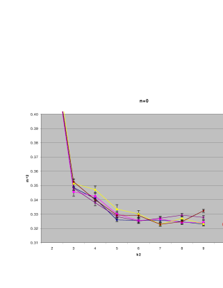
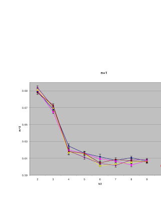
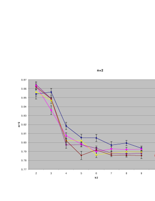
3 Determining the Cutoff

In this theory, the only dimensionful parameter is the cutoff, $\Lambda$. The cutoff can be determined by fitting the mass of one state. Explicitly, if we fix the cutoff using the $i^{th}$ state we find:

$$\Lambda^{2}=\frac{m^{2}_{\mathrm{measured}}}{\langle i|{\cal M}^{2}(\Lambda)|i\rangle},$$ (77)

where $m^{2}_{\mathrm{measured}}$ is the measured mass-squared for the state. There is no real experimental data for glueballs, so we use lattice results [40] for the “measured” values. Figure 4 shows how the coupling and cutoff are related when we fix the first excited state.

Figure 4: The coupling $\alpha$ as a function of the cutoff $\Lambda$, in units of the first excited state mass when the first excited state is fixed.

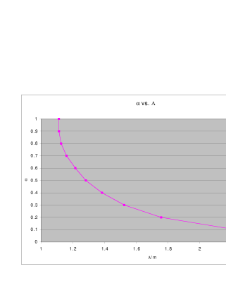
Figure 5 shows that when we fix the first excited state, for $\alpha=.5$, $k1=6$ and $k2=6$ the value of the cutoff has converged.

Figure 5: The cutoff for a few values of $k2$ when $\alpha=.5$. This shows the result is converged.

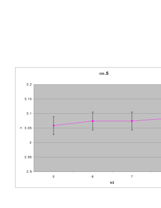
4 Masses versus Coupling

In this section we show how the masses depend on the coupling, $\alpha$, when the first excited state is fixed. However in these plots rather than showing the mass’s dependence on the coupling, we show its dependence on the cutoff. These plots help determine for what range of cutoffs the masses have a small cutoff dependence to determine where the theory is least cutoff dependent. In agreement with Allen’s results [26, 27], we find the slowest cutoff dependence for $.5\leq\alpha\leq.7$.

In figures 6 through 8 the masses are plotted as a function of the cutoff when the first excited state is fixed. This is equivalent to plotting the masses as a function of the coupling.

Figure 6: Masses for j=0 states as a function of the cutoff when the first excited state is fixed.

Figure 7: Masses for j=1 states as a function of the cutoff when the first excited state is fixed.

Figure 8: Masses for j=2 states as a function of the cutoff when the first excited state is fixed.

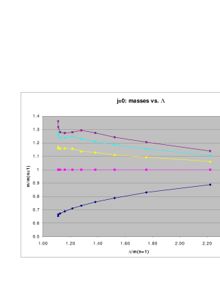
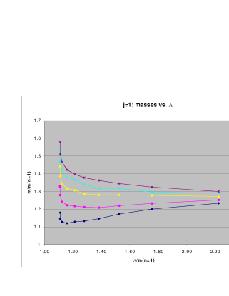
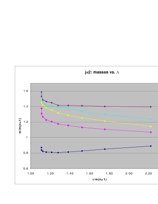
5 Glueball Spectrum

For completeness we present the glueball spectrum from [27] in this section. Our results are identical to within statistical errors to these previous results.

States are identified by $J^{PC}_{j}$ where $J$ is the total spin of the state, $j$ is the spin projection along the 3-axis, $P$ is the parity of the state, and $C$ is the state’s charge conjugation eigenvalue. An asterisk in the state notation next to the value of $C$ denotes an excited state with the given quantum numbers. Finally, we need to distinguish states with identical $J$’s and $P$’s and different $j$’s because we do not have manifest rotational symmetry. If $J=0$, we omit the subscript $j$ in the state notation.

Table 1 lists the glueball masses for $\alpha=.5$, in units of the mass of the ground state (the $0^{++}$ state). It also gives the average of lattice results from a number of different calculations for the sake of comparison [40]. The uncertainties listed are only statistical errors due to the Monte-Carlo integration. Finally, the three masses listed for the $J=2$ states correspond to $j=0,1,2$, where $j$ is the spin projection along the 3-axis.

State $M/M_{0^{++}}$ Lattice [40] $0^{-+}$ $1.38\pm 0.02$ $1.34\pm 0.18$ $1.58\pm 0.01$ $2^{++}$ $1.58\pm 0.02$ $1.42\pm 0.06$ $1.11\pm 0.01$ $1.70\pm 0.01$ $2^{++*}$ $1.68\pm 0.02$ $1.85\pm 0.20$ $1.62\pm 0.02$ $0^{++*}$ $1.77\pm 0.02$ $1.78\pm 0.12$

Table 1: The glueball masses from [27], which are identical to our masses within statistical errors, compared to an average of lattice results from a number of different calculations [40]. Masses are in units of the mass of the $0^{++}$ state. The uncertainties are only the statistical uncertainties associated with the Monte Carlo evaluation of the matrix elements of ${\cal M}^{2}(\Lambda)$. The three values of the masses for the $2^{++}$ and $2^{++*}$ states for our calculation correspond to $j=0,1,2$. We use $\alpha=0.5$, with 8 longitudinal (4 symmetric and 4 antisymmetric) basis functions, 7 transverse-magnitude basis functions, and 4 spin basis functions, for a total of 112 basis functions.

6 Wavefunction Plots

In this section we plot the spin-averaged probability density for the glueballs which is defined in Eq. (72) for states some of the low-lying states with $j=0$ and $j=1$. We only show a few functions since they are similar to those found in [26, 27]. The variable “$x\_plt$” is the longitudinal momentum fraction for one of the gluons, and the variable “$k\_plt$” is the relative transverse momentum of the state in units of the cutoff.

Figures 9 through 12 show the probability density for four of the the low-lying glueball states. Each wavefunction is built from 8 longitudinal (4 symmetric and 4 antisymmetric) basis functions and 7 transverse functions. Including the four spin states, there are 112 basis states.

Figure 9: Wavefunction for the $0^{++}$ glueball with $\alpha=\frac{1}{2}$.

Figure 10: Wavefunction for the $0^{-+}$ glueball with $\alpha=\frac{1}{2}$.

Figure 11: Wavefunction for the $2^{++}_{0}$ glueball with $\alpha=\frac{1}{2}$.

Figure 12: Wavefunction for the $2^{++}_{0}$ glueball with $\alpha=\frac{1}{2}$.

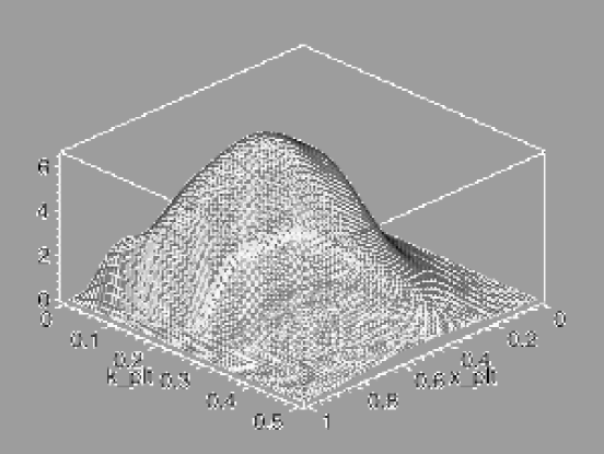
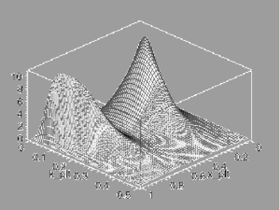
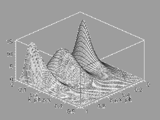
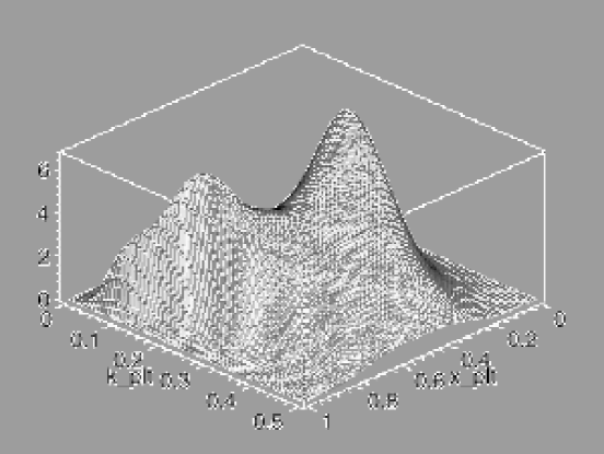
Chapter 6 Matrix Elements of the Approximate Meson States

We calculate all of the matrix elements of the approximate IMO (introduced in Section 6) necessary for a second-order calculation. The matrix elements are divided into four types of contributions; kinetic energy (KE), self-energy (SE), exchange (EX) and instantaneous exchange (IN). The four contributions are combined to explicitly cancel divergences (discussed in Section 7). With this division the full expression can be written:

$$\langle q^{\prime},l^{\prime},t^{\prime},j^{\prime}|{\cal M}^{2}(\Lambda)|q,l,t,j\rangle = \langle q^{\prime},l^{\prime},t^{\prime},j^{\prime}|{\cal M}^{2}(\Lambda)|q,l,t,j\rangle_{\mathrm{KE}}$$ (1)

$$+ \langle q^{\prime},l^{\prime},t^{\prime},j^{\prime}|{\cal M}^{2}(\Lambda)|q,l,t,j\rangle_{\mathrm{SE}}^{\mathrm{F}}$$

$$+ \langle q^{\prime},l^{\prime},t^{\prime},j^{\prime}|{\cal M}^{2}(\Lambda)|q,l,t,j\rangle_{\mathrm{EX}}^{\mathrm{F}}$$

$$+ \langle q^{\prime},l^{\prime},t^{\prime},j^{\prime}|{\cal M}^{2}(\Lambda)|q,l,t,j\rangle_{\mathrm{IN+EX}}$$

$$+ \langle q^{\prime},l^{\prime},t^{\prime},j^{\prime}|{\cal M}^{2}(\Lambda)|q,l,t,j\rangle_{\mathrm{IN}}^{\mathrm{B,F}},$$

where the free-state functions $|q,l,t,j\rangle$ are defined in Eq. (47). In the remainder of this Chapter we determine the matrix elements that need to be calculated by numerical integration. The integrals are divided into two groups: two-dimensional and five-dimensional.

1 Two-Dimensional Integrals

1 The Kinetic Energy

The two-dimensional integral for the kinetic energy is very similar to the overlap integral. The only difference in the derivation is:

$$\langle q^{\prime}_{1}\bar{q}^{\prime}_{2}|q_{1}\bar{q}_{2}\rangle\rightarrow\frac{\vec{k}^{2}+m^{2}}{x(1-x)}\langle q^{\prime}_{1}\bar{q}^{\prime}_{2}|q_{1}\bar{q}_{2}\rangle.$$ (2)

Thus, we have:

$$\langle q^{\prime},l^{\prime},t^{\prime},j^{\prime}|{\cal M}^{2}(\Lambda)|q,l,t,j\rangle_{\mathrm{KE}}=2\Lambda^{2}\delta_{q,q^{\prime}}\delta_{j,j^{\prime}}\int_{-1}^{1}\frac{dy_{k}}{(1+y_{k})^{2}}\left(\frac{2}{1+y_{k}}-1\right)$$

$$\hskip 56.9055pt\times\left[\left(\frac{2}{1+y_{k}}-1\right)^{2}+m^{2}\right]B_{t}(y_{k})B_{t^{\prime}}(y_{k})\int_{0}^{1}dx\frac{B_{l}(x)B_{l^{\prime}}(x)}{x(1-x)}.$$ (3)

2 The Self Energy

We need to separate Eq. (3) into divergent and finite pieces:

$$\langle q_{3}\bar{q}_{4}|V^{(2)}_{\mathrm{SE}}(\Lambda)|q_{1}\bar{q}_{2}\rangle=$$

$$\hskip 28.45274pt-\frac{\delta_{1,3}\delta_{2,4}}{24\pi^{2}}\Lambda^{2}\left[\int\frac{z\hskip 2.84544ptdz}{1-z}\left\{\frac{1+z^{2}}{z}\sqrt{2\pi}\left[\mathrm{erf}\left(\gamma(x,z)\right)+\mathrm{erf}\left(\gamma(1-x,z)\right)-2\right]\right.\right.$$

$$\hskip 42.67912pt\left.\left.+\sqrt{8}\left[\gamma(x,z)\mathrm{Ei}\left(1,\gamma^{2}(x,z)\right)+\gamma(1-x,z)\mathrm{Ei}\left(1,\gamma^{2}(1-x,z)\right)\right]\right\}\right].$$ (4)

The divergent part of the self-energy is contained in the term:

$$-\frac{\delta_{1,3}\delta_{2,4}}{24\pi^{2}}\Lambda^{2}\int dz\frac{1+z^{2}}{1-z}\left(-2\sqrt{2\pi}\right)=-2\sqrt{2\pi}\frac{\delta_{1,3}\delta_{2,4}}{24\pi^{2}}\Lambda^{2}\left[2\log(\epsilon)+\frac{3}{2}\right].$$ (5)

So now we can split the self-energy contribution into a finite and divergent piece:

$$\langle q_{3}\bar{q}_{4}|V^{(2)}_{\mathrm{SE}}(\Lambda)|q_{1}\bar{q}_{2}\rangle^{\mathrm{F}}=-\frac{\delta_{1,3}\delta_{2,4}}{24\pi^{2}}\Lambda^{2}$$

$$\hskip 28.45274pt\left[\int\frac{z\hskip 2.84544ptdz}{1-z}\left\{\frac{1+z^{2}}{z}\sqrt{2\pi}\left[\mathrm{erf}\left(\gamma(x,z)\right)+\mathrm{erf}\left(\gamma(1-x,z)\right)\right]\right.\right.$$

$$\hskip 85.35826pt\left.\left.+\sqrt{8}\left[\gamma(x,z)\mathrm{Ei}\left(1,\gamma^{2}(x,z)\right)\right.\right.\right.$$

$$\hskip 113.81102pt\left.\left.\left.+\gamma(1-x,z)\mathrm{Ei}\left(1,\gamma^{2}(1-x,z)\right)\right]\right\}+3\sqrt{2\pi}\right],$$ (6)

$$\langle q_{3}\bar{q}_{4}|V^{(2)}_{\mathrm{SE}}(\Lambda)|q_{1}\bar{q}_{2}\rangle^{\mathrm{D}}=-\frac{\delta_{1,3}\delta_{2,4}}{24\pi^{2}}\Lambda^{2}4\sqrt{2\pi}\log(\epsilon),$$ (7)

with

$$\langle q^{\prime},l^{\prime},t^{\prime},j^{\prime}|{\cal M}^{2}(\Lambda)|q,l,t,j\rangle_{\mathrm{SE}}^{\mathrm{F}}=g_{\Lambda}^{2}e^{-\Lambda^{-4}\Delta^{2}_{FI}}\langle q^{\prime},l^{\prime},t^{\prime},j^{\prime}|V^{(2)}_{\mathrm{SE}}(\Lambda)|q,l,t,j\rangle^{\mathrm{F}},$$ (8)

$$\langle q^{\prime},l^{\prime},t^{\prime},j^{\prime}|{\cal M}^{2}(\Lambda)|q,l,t,j\rangle_{\mathrm{SE}}^{\mathrm{D}}=g_{\Lambda}^{2}e^{-\Lambda^{-4}\Delta^{2}_{FI}}\langle q^{\prime},l^{\prime},t^{\prime},j^{\prime}|V^{(2)}_{\mathrm{SE}}(\Lambda)|q,l,t,j\rangle^{\mathrm{D}}.$$ (9)

We find for the finite part (see Eq. 47):

$$\langle q^{\prime},l^{\prime},t^{\prime},j{\cal M}^{2}(\Lambda)|q,l,t,j\rangle^{\mathrm{F}}_{\mathrm{SE}}=16\pi^{3}g_{\Lambda}^{2}{\cal P}^{+}\delta^{(3)}({\cal P}-{\cal P}^{\prime})\delta_{q,q^{\prime}}\delta_{j,j^{\prime}}\Lambda^{2}$$

$$\hskip 56.9055pt\times\left(-\frac{1}{24\pi^{2}}\right)\int_{0}^{1}dxB_{l}(x)B_{l^{\prime}}(x){\mathrm{I}}(x)\int_{0}^{\infty}dq\hskip 2.84544ptq\tilde{B}_{t}(q)\tilde{B}_{t^{\prime}}(q),$$ (10)

where

$$\mathrm{I}(x)=3\sqrt{2\pi}+\int\frac{z\hskip 2.84544ptdz}{1-z}\left\{\frac{1+z^{2}}{z}\sqrt{2\pi}\left[\mathrm{erf}\left(\gamma(x,z)\right)+\mathrm{erf}\left(\gamma(1-x,z)\right)\right]\right.$$

$$\hskip 113.81102pt\left.+\sqrt{8}\left[\gamma(x,z)\mathrm{Ei}\left(1,\gamma^{2}(x,z)\right)\right.\right.$$

$$\hskip 170.71652pt\left.\left.+\gamma(1-x,z)\mathrm{Ei}\left(1,\gamma^{2}(1-x,z)\right)\right]\right\}.$$ (11)

The divergent part of the self-energy is identical, except:

$$\mathrm{I}(x)\rightarrow 4\sqrt{2\pi}\log(\epsilon),$$ (12)

giving

$$\langle q^{\prime},l^{\prime},t^{\prime},j|{\cal M}^{2}(\Lambda)|q,l,t,j\rangle^{\mathrm{D}}_{\mathrm{SE}}=-\frac{4}{3}(2\pi)^{\frac{3}{2}}\Lambda^{2}\log(\epsilon)\hskip 2.84544ptg_{\Lambda}^{2}{\cal P}^{+}\delta^{(3)}({\cal P}-{\cal P}^{\prime})$$

$$\hskip 85.35826pt\times\delta_{q,q^{\prime}}\delta_{j,j^{\prime}}\int_{0}^{1}dxB_{l}(x)B_{l^{\prime}}(x)\int_{0}^{\infty}dq\hskip 2.84544ptq\tilde{B}_{t}(q)\tilde{B}_{t^{\prime}}(q).$$ (13)

2 Five-Dimensional Integrals

1 The Instantaneous Interaction

The matrix element of the instantaneous interaction in the approximate basis is given by:

$$\langle q^{\prime},l^{\prime},t^{\prime},j^{\prime}|{\cal M}^{2}(\Lambda)|q,l,t,j\rangle_{\mathrm{IN}}=g_{\Lambda}^{2}e^{-\Lambda^{-4}\Delta_{FI}^{2}}\times$$

$$\hskip 28.45274pt\frac{1}{16\pi^{3}}\frac{1}{N_{c}}\sum_{s_{1\rightarrow 4},c_{1\rightarrow 4}}\int\frac{d^{2}\vec{q}dx}{\sqrt{x(1-x)}}\int\frac{d^{2}\vec{p}dy}{\sqrt{y(1-y)}}\theta_{\epsilon}\theta_{\epsilon^{\prime}}\delta_{c_{1},c_{2}}\delta_{c_{3},c_{4}}\chi_{q}^{s_{1}s_{2}}\chi_{q^{\prime}}^{s_{3}s_{4}}\times$$

$$\hskip 28.45274ptB_{l^{\prime}}(y)B_{l}(x)\tilde{B}_{t}(q)\tilde{B}_{t^{\prime}}(p)A^{\ast}_{j^{\prime}-s_{3}-s_{4}}(\phi^{\prime})A_{j-s_{1}-s_{2}}(\phi)\langle q_{3}\bar{q}_{4}|V_{\mathrm{IN}}^{(2)}(\Lambda)|q_{1}\bar{q}_{2}\rangle,$$ (14)

where the matrix element of the reduced interaction is defined in Eq. (2). This can be reduced to:

$$\langle q^{\prime},l^{\prime},t^{\prime},j^{\prime}|{\cal M}^{2}(\Lambda)|q,l,t,j\rangle_{\mathrm{IN}}=$$

$$\hskip 28.45274pt-\frac{32}{N_{c}}g_{\Lambda}^{2}{\cal P}^{+}\delta({\cal P}-{\cal P}^{\prime})\delta_{j,j^{\prime}}\int d\gamma_{\phi}dqqdx\int dppdy\theta_{\epsilon}\theta_{\epsilon^{\prime}}$$

$$\hskip 56.9055pt\times\theta(x-y-\epsilon)B_{l^{\prime}}(y)B_{l}(x)\tilde{B}_{t}(q)\tilde{B}_{t^{\prime}}(p)\frac{e^{-\Lambda^{-4}\Delta_{FI}^{2}}}{(x-y)^{2}}$$

$$\hskip 85.35826pt\times\left[\delta_{q,1}\delta_{q^{\prime},1}\cos([j-1]\gamma_{\phi})+\delta_{q,2}\delta_{q^{\prime},2}\cos([j+1]\gamma_{\phi})\right.$$

$$\hskip 170.71652pt\left.+\left(\delta_{q,3}\delta_{q^{\prime},3}+\delta_{q,4}\delta_{q^{\prime},4}\right)\cos(j\gamma_{\phi})\right].$$ (15)

Finally, as discussed in Section 7, we split the instantaneous interaction into two parts, a part above the cutoff that vanishes in the limit $\Lambda\rightarrow\infty$, and a part below the cutoff that remains in this limit:

$$\langle q^{\prime},l^{\prime},t^{\prime},j^{\prime}|{\cal M}^{2}(\Lambda)|q,l,t,j\rangle^{\mathrm{A}}_{\mathrm{IN}} = \left[1-e^{2\Lambda^{-4}\Delta_{FK}^{(1)}\Delta_{KI}^{(1)}}\right]$$ (16)

$$\hskip 28.45274pt\times\langle q^{\prime},l^{\prime},t^{\prime},j^{\prime}|{\cal M}^{2}(\Lambda)|q,l,t,j\rangle_{\mathrm{IN}},$$

$$\langle q^{\prime},l^{\prime},t^{\prime},j^{\prime}|{\cal M}^{2}(\Lambda)|q,l,t,j\rangle^{\mathrm{B}}_{\mathrm{IN}} = e^{2\Lambda^{-4}\Delta_{FK}^{(1)}\Delta_{KI}^{(1)}}$$ (17)

$$\hskip 28.45274pt\times\langle q^{\prime},l^{\prime},t^{\prime},j^{\prime}|{\cal M}^{2}(\Lambda)|q,l,t,j\rangle_{\mathrm{IN}}.$$

2 The Finite Part of the Exchange Interaction

The matrix element of the finite part of the exchange interaction is:

$$\langle q^{\prime},l^{\prime},t^{\prime},j^{\prime}|{\cal M}^{2}(\Lambda)|q,l,t,j\rangle_{\mathrm{EX}}=g_{\Lambda}^{2}e^{-\Lambda^{-4}\Delta_{FI}^{2}}\times$$

$$\hskip 28.45274pt\frac{1}{16\pi^{3}}\frac{1}{N_{c}}\sum_{s_{1\rightarrow 4},c_{1\rightarrow 4}}\int\frac{d^{2}\vec{q}dx}{\sqrt{x(1-x)}}\int\frac{d^{2}\vec{p}dy}{\sqrt{y(1-y)}}\theta_{\epsilon}\theta_{\epsilon^{\prime}}\delta_{c_{1},c_{2}}\delta_{c_{3},c_{4}}\chi_{q}^{s_{1}s_{2}}\chi_{q^{\prime}}^{s_{3}s_{4}}\times$$

$$\hskip 28.45274ptB_{l^{\prime}}(y)B_{l}(x)\tilde{B}_{t}(q)\tilde{B}_{t^{\prime}}(p)A^{\ast}_{j^{\prime}-s_{3}-s_{4}}(\phi^{\prime})A_{j-s_{1}-s_{2}}(\phi)\langle q_{3}\bar{q}_{4}|V_{\mathrm{EX}}^{(2)}(\Lambda)|q_{1}\bar{q}_{2}\rangle,$$ (18)

where the matrix element is given in Eq. (2). After many pages of algebra the contribution from the finite part of the exchange interaction is given by:

$$\langle q^{\prime},l^{\prime},t^{\prime},j^{\prime}|{\cal M}^{2}(\Lambda)|q,l,t,j\rangle^{\mathrm{F}}_{\mathrm{EX}}=-{\cal P}^{+}\delta^{3}({\cal P}-{\cal P}^{\prime})\left(N_{c}-\frac{1}{3}\right)\theta(x-y-\epsilon)\times$$

$$\hskip 36.135ptg_{\Lambda}^{2}e^{-\Lambda^{-4}\Delta_{FI}^{2}}\int d\gamma_{\phi}dqqdx\int dppdy\frac{1}{x-y}\frac{B_{l^{\prime}}(y)B_{l}(x)\tilde{B}_{t}(q)\tilde{B}_{t^{\prime}}(p)}{x(1-x)y(1-y)}$$

$$\hskip 113.81102pt\times\left(\frac{1}{\Delta_{FK}^{(1)}}-\frac{1}{\Delta_{KI}^{(1)}}\right)\left[1-e^{2\Lambda^{-4}\Delta_{FK}^{(1)}\Delta_{KI}^{(1)}}\right]\delta_{j,j^{\prime}}S_{q,q^{\prime}},$$ (19)

where the $S_{q,q^{\prime}}$ are given by:

$$S_{1,1} = -\frac{1}{x-y}\left[q^{2}y(1-y)(1-2x)-p^{2}x(1-x)(1-2y)\right]\cos([j-1]\gamma_{\phi})$$

$$\hskip 85.35826pt-pq\left[y^{2}(1-2x)-x^{2}(1-2y)-2y(1-x)\right]\cos(j\gamma_{\phi}),$$

$$S_{2,2} = -\frac{1}{x-y}\left[q^{2}y(1-y)(1-2x)-p^{2}x(1-x)(1-2y)\right]\cos([j+1]\gamma_{\phi})$$

$$\hskip 85.35826pt-pq\left[y^{2}(1-2x)-x^{2}(1-2y)-2y(1-x)\right]\cos(j\gamma_{\phi}),$$

$$S_{3,3} = -\cos(j\gamma_{\phi})\left[pq\cos\gamma_{\phi}(1-x-y+2xy)\right.$$

$$\hskip 56.9055pt\left.-\frac{1-x-y}{x-y}\left(y(1-y)q^{2}-x(1-x)p^{2}\right)-m^{2}(x-y)^{2}\right],$$

$$S_{4,4} = -\cos(j\gamma_{\phi})\left[pq\cos\gamma_{\phi}(1-x-y+2xy)\right.$$

$$\hskip 56.9055pt\left.-\frac{1-x-y}{x-y}\left(y(1-y)q^{2}-x(1-x)p^{2}\right)+m^{2}(x-y)^{2}\right],$$

$$S_{1,2} = 0,$$

$$S_{2,1} = 0,$$

$$S_{1,3} = \frac{im}{\sqrt{2}}\left[(1-2y)q\cos(j\gamma_{\phi})-(1-x-y)p\cos([j-1]\gamma_{\phi})\right],$$

$$S_{3,1} = \frac{im}{\sqrt{2}}\left[(1-x-y)q\cos([j-1]\gamma_{\phi})-(1-2x)p\cos(j\gamma_{\phi})\right],$$

$$S_{1,4} = \frac{im}{\sqrt{2}}\left[-(1-2y+2y^{2})q\cos(j\gamma_{\phi})+(1-y-x+2xy)p\cos([j-1]\gamma_{\phi})\right],$$

$$S_{4,1} = \frac{im}{\sqrt{2}}\left[(1-2x+2x^{2})p\cos(j\gamma_{\phi})-(1-x-y+2xy)q\cos([j-1]\gamma_{\phi})\right],$$

$$S_{2,3} = \frac{im}{\sqrt{2}}\left[(1-2y)q\cos(j\gamma_{\phi})-(1-x-y)p\cos([j+1]\gamma_{\phi})\right],$$

$$S_{3,2} = \frac{im}{\sqrt{2}}\left[(1-x-y)q\cos([j+1]\gamma_{\phi})-(1-2x)p\cos(j\gamma_{\phi})\right],$$

$$S_{2,4} = \frac{im}{\sqrt{2}}\left[(1-2y+2y^{2})q\cos(j\gamma_{\phi})-(1-y-x+2xy)p\cos([j+1]\gamma_{\phi})\right],$$

$$S_{4,2} = \frac{im}{\sqrt{2}}\left[(1-x-y+2xy)q\cos([j+1]\gamma_{\phi})-(1-2x+2x^{2})p\cos(j\gamma_{\phi})\right],$$

$$S_{3,4} = \sqrt{2}pq\sin\gamma_{\phi}\sin(j\gamma_{\phi})(1-x-y),$$

$$S_{4,3} = \sqrt{2}pq\sin\gamma_{\phi}\sin(j\gamma_{\phi})(1-x-y).$$

3 The Divergent Part of the Exchange Interaction

The complete contribution from the divergent part of the exchange diagrams is:

$$\langle q^{\prime},l^{\prime},t^{\prime},j^{\prime}|{\cal M}^{2}(\Lambda)|q,l,t,j\rangle^{\mathrm{D}}_{\mathrm{EX}}=$$

$$\hskip 28.45274pt-2g_{\Lambda}^{2}e^{-\Lambda^{-4}\Delta_{FI}^{2}}{\cal P}^{+}\delta^{3}({\cal P}-{\cal P}^{\prime})\delta_{j,j^{\prime}}\left(N_{c}-\frac{1}{3}\right)$$

$$\hskip 42.67912pt\times\int d\gamma_{\phi}dqqdx\int dppdy\frac{\theta(x-y-\epsilon)}{x-y}B_{l^{\prime}}(y)B_{l}(x)\tilde{B}_{t}(q)\tilde{B}_{t^{\prime}}(p)$$

$$\hskip 56.9055pt\times\left(\frac{1}{\Delta_{FK}^{(1)}}-\frac{1}{\Delta_{KI}^{(1)}}\right)\left[1-e^{2\Lambda^{-4}\Delta_{FK}^{(1)}\Delta_{KI}^{(1)}}\right]\left\{\frac{p^{2}+q^{2}-2pq\cos(\gamma_{\phi})}{(x-y)^{2}}\right\}$$

$$\hskip 56.9055pt\times\left[\delta_{q,1}\delta_{q^{\prime},1}\cos([j-1]\gamma_{\phi})+\delta_{q,2}\delta_{q^{\prime},2}\cos([j+1]\gamma_{\phi})\right.$$

$$\hskip 142.26378pt\left.+\delta_{q,3}\delta_{q^{\prime},3}\cos(j\gamma_{\phi})+\delta_{q,4}\delta_{q^{\prime},4}\cos(j\gamma_{\phi})\right].$$ (20)

4 Combining the Divergent Part of the Exchange Interaction and the Instantaneous Interaction Above the Cutoff

If we consider the contribution from the instantaneous interaction above the cutoff (Eq. 16) and the divergent part of the exchange interaction (Eq. 3), we see that in the limit $x=y$ the two divergent contributions cancel. Thus, we can combine the two interactions and write them as:

$$\langle q^{\prime},l^{\prime},t^{\prime},j^{\prime}|{\cal M}^{2}(\Lambda)|q,l,t,j\rangle_{\mathrm{IN+EX}}=$$

$$\hskip 28.45274pt-\frac{16}{3}g_{\Lambda}^{2}{\cal P}^{+}\delta({\cal P}-{\cal P}^{\prime})\delta_{j,j^{\prime}}$$

$$\hskip 56.9055pt\int d\gamma_{\phi}dqqdx\int dppdy\theta_{\epsilon}\theta_{\epsilon^{\prime}}\theta(x-y-\epsilon)e^{-\Lambda^{-4}\Delta_{FI}^{2}}$$

$$\hskip 42.67912pt\times B_{l^{\prime}}(y)B_{l}(x)\tilde{B}_{t}(q)\tilde{B}_{t^{\prime}}(p)\left[1-e^{2\Lambda^{-4}\Delta_{FK}^{(1)}\Delta_{KI}^{(1)}}\right]$$

$$\hskip 42.67912pt\times\left\{\frac{W_{q,q^{\prime}}}{(x-y)^{2}}\left[\left(\frac{1}{\Delta_{FK}^{(1)}}-\frac{1}{\Delta_{KI}^{(1)}}\right)\left(\frac{p^{2}+q^{2}-2\vec{p}\cdot\vec{q}}{x-y}\right)+2\right]\right\},$$ (21)

where

$$W_{q,q^{\prime}} = \delta_{q,1}\delta_{q^{\prime},1}\cos([j-1]\gamma_{\phi})+\delta_{q,2}\delta_{q^{\prime},2}\cos([j+1]\gamma_{\phi})$$ (22)

$$\hskip 142.26378pt+\left(\delta_{q,3}\delta_{q^{\prime},3}+\delta_{q,4}\delta_{q^{\prime},4}\right)\cos(j\gamma_{\phi}).$$

In the limit $|x-y|\rightarrow 0$ the term in square brackets (inside the braces) vanishes, leaving the entire term finite in this limit so we no longer need the infrared cutoff for this term.

5 Combining the Divergent Part of the Self-Energy and the Instantaneous Interaction Below the Cutoff

The combination of the instantaneous interaction below the cutoff and the divergent part of the self-energy is algebraically complex. The details of the calculation can be found in Appendix 11. We find:

$$\langle q^{\prime},l^{\prime},t^{\prime},j^{\prime}|{\cal M}^{2}(\Lambda)|q,l,t,j\rangle_{\mathrm{IN}}^{\mathrm{B,F}}=-g_{\Lambda}^{2}\frac{32}{3}\delta_{j,j^{\prime}}{\cal P}^{+}\delta({\cal P-P^{\prime}})\theta(x-y)\theta(x-y-\epsilon)$$

$$\int_{2\epsilon}^{1-\epsilon}dx\int_{\epsilon}^{x-\epsilon}dy\log(x-y)\int d^{2}\vec{q}d^{2}\vec{p}B_{l}(x)\tilde{B}_{t}(q)\tilde{B}_{t^{\prime}}(p)W_{q,q^{\prime}}e^{-\Lambda^{-4}(\Delta^{2}_{FK}+\Delta^{2}_{IK})}$$

$$\hskip 56.9055pt\times\left[\frac{B_{l^{\prime}}(y)}{(x-y)^{2}}+\frac{B^{\prime}_{l^{\prime}}(y)}{x-y}-2\frac{B_{l^{\prime}}(y)}{x-y}\left(\Delta_{FK}\Delta_{FK}^{\prime}+\Delta_{KI}\Delta_{KI}^{\prime}\right)\right],$$ (23)

where,

$$\Delta_{KI} = \frac{m^{2}(x-y)^{2}+(x\vec{p}-y\vec{q})^{2}}{xy(x-y)}$$

$$= \frac{m^{2}(x-y)-yq^{2}+xp^{2}}{xy}+\frac{(\vec{p}-\vec{q})^{2}}{x-y},$$

$$\Delta_{FK} = -\frac{m^{2}(x-y)^{2}+\left[(1-x)\vec{p}-(1-y)\vec{q}\hskip 2.84544pt\right]^{2}}{(1-x)(1-y)(x-y)}$$

$$= -\frac{m^{2}(x-y)+(1-y)q^{2}-(1-x)p^{2}}{(1-x)(1-y)}-\frac{(\vec{p}-\vec{q})^{2}}{x-y},$$

$$\Delta_{KI}^{\prime} = \frac{(\vec{p}-\vec{q})^{2}}{(x-y)^{2}}-\frac{m^{2}+p^{2}}{y^{2}},$$

$$\Delta_{FK}^{\prime} = \frac{m^{2}+p^{2}}{(1-y)^{2}}-\frac{(\vec{p}-\vec{q})^{2}}{(x-y)^{2}}.$$

However, the integrand has an apparent divergence as $x\rightarrow y$. The integrals over transverse momenta, however, integrate to zero in this case, killing the divergence. We can subtract a term that integrates to zero and that explicitly cancels the false divergence from the above contribution. We make the following change of variables to aid in the calculation of the term we want to subtract:

$$\vec{r}=\frac{1}{2}(\vec{p}+\vec{q}),\hskip 28.45274pt\vec{w}=\frac{1}{2}\frac{\vec{q}-\vec{p}}{\sqrt{\eta}},$$ (24)

where

$$\vec{r}=r\left[\cos\alpha\hat{x}+\sin\alpha\hat{y}\right],\hskip 28.45274pt\vec{w}=w\left[\cos\delta\hat{x}+\sin\delta\hat{y}\right]$$ (25)

and

$$\beta=\alpha-\delta,\hskip 28.45274pt\vec{r}\cdot\vec{w}=rw\cos\beta.$$ (26)

Then

$$\vec{q}=\vec{r}+\eta\vec{w},\hskip 28.45274pt\vec{p}=\vec{r}-\eta\vec{w},$$ (27)

and

$$q=\sqrt{r^{2}+\eta w^{2}+2rw\sqrt{\eta}\cos\beta},\hskip 28.45274ptp=\sqrt{r^{2}+\eta w^{2}-2rw\sqrt{\eta}\cos\beta}.$$ (28)

For convenience, we define:

$$r_{\pm}\equiv\sqrt{r^{2}+\eta w^{2}\pm 2rw\sqrt{\eta}\cos\beta}.$$ (29)

Finally,

$$\vec{q}\cdot\vec{p}=r^{2}-\eta w^{2},\hskip 28.45274pt\cos\gamma_{\phi}=\frac{r^{2}-\eta w^{2}}{r_{+}r_{-}},\hskip 28.45274pt\sin\gamma_{\phi}=\frac{-2rw\sqrt{\eta}}{r_{+}r_{-}}\sin\beta,$$ (30)

are useful relations. The details of this subtraction are in Appendix 11. After making the subtraction, we have:

$$\langle q^{\prime},l^{\prime},t^{\prime},j^{\prime}|{\cal M}^{2}(\Lambda)|q,l,t,j\rangle_{\mathrm{IN}}^{\mathrm{B,F}}=$$

$$\hskip 28.45274pt-g_{\Lambda}^{2}\frac{128}{3}\delta_{j,j^{\prime}}{\cal P}^{+}\delta({\cal P-P^{\prime}})\int_{0}^{1}dxB_{l}(x)\int_{0}^{x}dy\hskip 2.84544pt\eta\log\eta\int d^{2}\vec{r}d^{2}\vec{w}$$

$$\hskip 56.9055pt\times\left\{e^{-(\Delta^{2}_{FK}+\Delta^{2}_{IK})}W_{q,q^{\prime}}\tilde{B}_{t}(r_{+})\tilde{B}_{t^{\prime}}(r_{-})\left[\frac{B_{l^{\prime}}(y)}{\eta^{2}}+\frac{B^{\prime}_{l^{\prime}}(y)}{\eta}\right.\right.$$

$$\hskip 142.26378pt\left.\left.-2\frac{B_{l^{\prime}}(y)}{\eta}\left(\Delta_{FK}\Delta_{FK}^{\prime}+\Delta_{KI}\Delta_{KI}^{\prime}\right)\right]\right.$$

$$\hskip 113.81102pt\left.-\tilde{B}_{t}(r)\tilde{B}_{t^{\prime}}(r)B_{l^{\prime}}(y)\frac{\delta_{q,q^{\prime}}}{\eta^{2}}e^{-32w^{4}}\left[1-64w^{4}\right]\right\}.$$ (31)

The integral is explicitly finite, but still sharply peaked around $x\approx y$. We can speed convergence of the numerical integration by smoothing the integral using the change of variables:

$$\eta=xe^{-p},\hskip 28.45274ptdy=\eta dp,$$ (32)

and

$$y_{w}=\frac{2}{1+w}-1,\hskip 28.45274pty_{r}=\frac{2}{1+r}-1,\hskip 28.45274pty_{p}=\frac{2}{1+p}-1.$$ (33)

Finally, we get:

$$\langle q^{\prime},l^{\prime},t^{\prime},j^{\prime}|{\cal M}^{2}(\Lambda)|q,l,t,j\rangle_{\mathrm{IN}}^{\mathrm{B,F}}=$$

$$\hskip 28.45274pt-8g_{\Lambda}^{2}\frac{128}{3}\delta_{j,j^{\prime}}{\cal P}^{+}\delta({\cal P-P^{\prime}})$$

$$\hskip 56.9055pt\times\int_{0}^{1}dx\int_{0}^{2\pi}d\gamma_{\phi}\int_{-1}^{1}\frac{dy_{p}}{(1+y_{p})^{2}}\int_{-1}^{1}\frac{dy_{r}}{(1+y_{r})^{2}}\int_{-1}^{1}\frac{dy_{w}}{(1+y_{w})^{2}}$$

$$\hskip 56.9055pt\times\eta\log\eta\hskip 2.84544ptr\hskip 2.84544ptwB_{l}(x)$$

$$\hskip 56.9055pt\times\left\{e^{-(\Delta^{2}_{FK}+\Delta^{2}_{IK})}W_{q,q^{\prime}}\tilde{B}_{t}(r_{+})\tilde{B}_{t^{\prime}}(r_{-})\right.$$

$$\hskip 85.35826pt\left.\times\left[\frac{B_{l^{\prime}}(y)}{\eta}+B^{\prime}_{l^{\prime}}(y)-2B_{l^{\prime}}(y)\left(\Delta_{FK}\Delta_{FK}^{\prime}+\Delta_{KI}\Delta_{KI}^{\prime}\right)\right]\right.$$

$$\hskip 128.0374pt\left.-\tilde{B}_{t}(r)\tilde{B}_{t^{\prime}}(r)B_{l^{\prime}}(y)\frac{\delta_{q,q^{\prime}}}{\eta}e^{-32w^{4}}\left[1-64w^{4}\right]\right\},$$ (34)

where,

$$\Delta_{KI} = \frac{m^{2}\eta-yr_{+}^{2}+xr_{-}^{2}}{xy}+4w^{2},$$

$$\Delta_{FK} = -\frac{m^{2}\eta+(1-y)r_{+}^{2}-(1-x)r_{-}^{2}}{(1-x)(1-y)}-4w^{2},$$

$$\Delta_{KI}^{\prime} = \frac{4w^{2}}{\eta}-\frac{m^{2}+r_{-}^{2}}{y^{2}},$$

$$\Delta_{FK}^{\prime} = \frac{m^{2}+r_{-}^{2}}{(1-y)^{2}}-\frac{4w^{2}}{\eta}.$$

Chapter 7 Numerical Issues and Parallelization

With a problem of this nature the analytic calculation is only part of the solution. To get results that can be used to check the theory or make predictions, it is necessary to further refine the calculation for efficient numerical calculations. Furthermore we can obtain results more rapidly from a well-designed algorithm that makes the best use of computer resources.

In this chapter we discuss some of the refinements that help make the Monte-Carlo integration more efficient. We also describe the algorithm and how it is parallelized.

1 Numerical Calculation of Meson Mass Spectra

In order to aid the numerical calculations, we will use the change of variables given in Eq. (24) through Eq. (30) and Eq. (32) through Eq. (33). The complete change of variables gives:

$$\int_{0}^{x}dy\int_{0}^{\infty}dq\int_{0}^{\infty}dp\rightarrow 32\eta^{2}\int_{-1}^{1}\frac{dy_{s}}{(1+y_{s})^{2}}\int_{-1}^{1}\frac{dy_{w}}{(1+y_{w})^{2}}\int_{-1}^{1}\frac{dy_{r}}{(1+y_{r})^{2}}.$$ (1)

We divide out the common factor $16\pi^{3}{\cal P}^{+}\delta^{3}({\cal P}-{\cal P}^{\prime})$ from all the matrix elements and use the following definitions for all of the integrals:

$$W_{q,q^{\prime}}=\delta_{q,1}\delta_{q^{\prime},1}\cos([j-1]\gamma_{\phi})+\delta_{q,2}\delta_{q^{\prime},2}\cos([j+1]\gamma_{\phi})$$

$$\hskip 170.71652pt+\left(\delta_{q,3}\delta_{q^{\prime},3}+\delta_{q,4}\delta_{q^{\prime},4}\right)\cos(j\gamma_{\phi}),$$ (2)

$$\Delta_{FI} = \frac{m^{2}+r_{-}^{2}}{y(1-y)}-\frac{m^{2}+r_{+}^{2}}{x(1-x)}$$

$$= \frac{1}{x(1-x)y(1-y)}\left\{m^{2}\left[x(1-x)-y(1-y)\right]\right.$$

$$\hskip 28.45274pt\left.+\eta(1-x-y)\left(r^{2}+\eta w^{2}\right)\right.$$

$$\hskip 56.9055pt\left.-2rw\sqrt{\eta}\cos\beta\left[x(1-x)+y(1-y)\right]\right\},$$

$$\Delta_{KI} = \frac{m^{2}\eta-yr_{+}^{2}+xr_{-}^{2}}{xy}+4w^{2}$$

$$= \frac{\eta m^{2}+\eta\left(r^{2}+\eta w^{2}\right)-2rw\sqrt{\eta}\cos\beta(x+y)}{xy}+4w^{2},$$

$$\Delta_{FK} = -\frac{m^{2}\eta+(1-y)r_{+}^{2}-(1-x)r_{-}^{2}}{(1-x)(1-y)}-4w^{2}$$

$$= -\frac{\eta m^{2}+\eta\left(r^{2}+\eta w^{2}\right)+2rw\sqrt{\eta}\cos\beta\left(1-x+1-y\right)}{(1-x)(1-y)}-4w^{2},$$

$$\bar{\Delta}_{KI}^{\prime} = 4w^{2}-\eta\frac{m^{2}+r_{-}^{2}}{y^{2}},$$

$$\bar{\Delta}_{FK}^{\prime} = \eta\frac{m^{2}+r_{-}^{2}}{(1-y)^{2}}-4w^{2},$$ (3)

where we have rewritten some of the definitions to reduce round-off error. When calculating the cosine and sine functions of $\gamma_{\phi}$, we will need to use recursion relations since we can really only calculate $\sin\gamma_{\phi}$ and $\cos\gamma_{\phi}$ [see Eq. (30)].

1 The Finite Part of the Exchange Interaction

From Eq. (2) we get:

$$\langle q^{\prime},l^{\prime},t^{\prime},j^{\prime}|{\cal M}^{2}(\Lambda)|q,l,t,j\rangle^{\mathrm{F}}_{\mathrm{EX}}=$$

$$\hskip 28.45274pt-\frac{1}{6\pi^{3}}g_{\Lambda}^{2}\int d\gamma_{\phi}dqqdx\int dppdy\frac{e^{-\Delta_{FI}^{2}}}{x-y}\delta_{j,j^{\prime}}S_{q,q^{\prime}}$$

$$\hskip 56.9055pt\times\frac{B_{l^{\prime}}(y)B_{l}(x)\tilde{B}_{t}(q)\tilde{B}_{t^{\prime}}(p)}{x(1-x)y(1-y)}\left(\frac{1}{\Delta_{FK}}-\frac{1}{\Delta_{KI}}\right)\left[1-e^{2\Delta_{FK}\Delta_{KI}}\right]$$

$$=-\frac{16}{3\pi^{3}}g_{\Lambda}^{2}\delta_{j,j^{\prime}}\int_{0}^{1}dx\int_{0}^{2\pi}d\gamma_{\phi}\int_{-1}^{1}\frac{dy_{s}}{(1+y_{s})^{2}}\int_{-1}^{1}\frac{dy_{w}}{(1+y_{w})^{2}}\int_{-1}^{1}\frac{dy_{r}}{(1+y_{r})^{2}}$$

$$\hskip 56.9055pt\times\frac{B_{l^{\prime}}(y)B_{l}(x)B_{t}(y_{r_{+}})B_{t^{\prime}}(y_{r_{-}})}{x(1-x)y(1-y)}rwe^{-\Delta_{FI}^{2}}\left(\frac{1}{\Delta_{FK}}-\frac{1}{\Delta_{KI}}\right)$$

$$\hskip 113.81102pt\times\left[1-e^{2\Delta_{FK}\Delta_{KI}}\right]\bar{S}_{q,q^{\prime}},$$ (4)

where

$$y_{r_{\pm}}=\frac{2}{1+r_{\pm}}-1,$$ (5)

and:

$$\bar{S}_{1,1} = -\left[r_{+}^{2}y(1-y)(1-2x)-r_{-}^{2}x(1-x)(1-2y)\right]\cos([j-1]\gamma_{\phi})$$

$$\hskip 28.45274pt-\eta\hskip 2.84544ptr_{-}r_{+}\left[y^{2}(1-2x)-x^{2}(1-2y)-2y(1-x)\right]\cos(j\gamma_{\phi}),$$

$$\bar{S}_{2,2} = -\left[r_{+}^{2}y(1-y)(1-2x)-r_{-}^{2}x(1-x)(1-2y)\right]\cos([j+1]\gamma_{\phi})$$

$$\hskip 28.45274pt-\eta\hskip 2.84544ptr_{-}r_{+}\left[y^{2}(1-2x)-x^{2}(1-2y)-2y(1-x)\right]\cos(j\gamma_{\phi}),$$

$$\bar{S}_{3,3} = -\cos(j\gamma_{\phi})\left[\eta r_{-}r_{+}\cos\gamma_{\phi}(1-x-y+2xy)\right.$$

$$\hskip 56.9055pt\left.-(1-x-y)\left(y(1-y)r_{+}^{2}-x(1-x)r_{-}^{2}\right)-m^{2}\eta^{3}\right],$$

$$\bar{S}_{4,4} = -\cos(j\gamma_{\phi})\left[\eta r_{-}r_{+}\cos\gamma_{\phi}(1-x-y+2xy)\right.$$

$$\hskip 56.9055pt\left.-(1-x-y)\left(y(1-y)r_{+}^{2}-x(1-x)r_{-}^{2}\right)+m^{2}\eta^{3}\right],$$

$$\bar{S}_{1,2} = 0,$$

$$\bar{S}_{2,1} = 0,$$

$$\bar{S}_{1,3} = \frac{im\eta}{\sqrt{2}}\left[(1-2y)r_{+}\cos(j\gamma_{\phi})-(1-x-y)r_{-}\cos([j-1]\gamma_{\phi})\right],$$

$$\bar{S}_{3,1} = \frac{im\eta}{\sqrt{2}}\left[(1-x-y)r_{+}\cos([j-1]\gamma_{\phi})-(1-2x)r_{-}\cos(j\gamma_{\phi})\right],$$

$$\bar{S}_{1,4} = \frac{im\eta}{\sqrt{2}}\left[-(1-2y+2y^{2})r_{+}\cos(j\gamma_{\phi})\right.$$

$$\hskip 85.35826pt\left.+(1-y-x+2xy)r_{-}\cos([j-1]\gamma_{\phi})\right],$$

$$\bar{S}_{4,1} = \frac{im\eta}{\sqrt{2}}\left[(1-2x+2x^{2})r_{-}\cos(j\gamma_{\phi})\right.$$

$$\hskip 85.35826pt\left.-(1-x-y+2xy)r_{+}\cos([j-1]\gamma_{\phi})\right],$$

$$\bar{S}_{2,3} = \frac{im\eta}{\sqrt{2}}\left[(1-2y)r_{+}\cos(j\gamma_{\phi})-(1-x-y)r_{-}\cos([j+1]\gamma_{\phi})\right],$$

$$\bar{S}_{3,2} = \frac{im\eta}{\sqrt{2}}\left[(1-x-y)r_{+}\cos([j+1]\gamma_{\phi})-(1-2x)r_{-}\cos(j\gamma_{\phi})\right],$$

$$\bar{S}_{2,4} = \frac{im\eta}{\sqrt{2}}\left[(1-2y+2y^{2})r_{+}\cos(j\gamma_{\phi})\right.$$

$$\hskip 85.35826pt\left.-(1-y-x+2xy)r_{-}\cos([j+1]\gamma_{\phi})\right],$$

$$\bar{S}_{4,2} = \frac{im\eta}{\sqrt{2}}\left[(1-x-y+2xy)r_{+}\cos([j+1]\gamma_{\phi})\right.$$

$$\hskip 85.35826pt\left.-(1-2x+2x^{2})r_{-}\cos(j\gamma_{\phi})\right],$$

$$\bar{S}_{3,4} = \eta\sqrt{2}r_{-}r_{+}\sin\gamma_{\phi}\sin(j\gamma_{\phi})(1-x-y),$$

$$\bar{S}_{4,3} = \eta\sqrt{2}r_{-}r_{+}\sin\gamma_{\phi}\sin(j\gamma_{\phi})(1-x-y).$$

2 The Instantaneous and Exchange Interaction

Eq. (4) gives:

$$\langle q^{\prime},l^{\prime},t^{\prime},j^{\prime}|{\cal M}^{2}(\Lambda)|q,l,t,j\rangle_{\mathrm{IN+EX}}={\cal P}^{+}g_{\Lambda}^{2}e^{-\Lambda^{-4}\Delta_{FI}^{2}}\times$$

$$\hskip 14.22636pt-\frac{16}{3}\delta({\cal P}-{\cal P}^{\prime})\delta_{j,j^{\prime}}\int d\gamma_{\phi}dqqdx\int dppdy\theta_{\epsilon}\theta_{\epsilon^{\prime}}B_{l^{\prime}}(y)B_{l}(x)\tilde{B}_{t}(q)\tilde{B}_{t^{\prime}}(p)$$

$$\hskip 56.9055pt\times\left[1-e^{2\Lambda^{-4}\Delta_{FK}^{(1)}\Delta_{KI}^{(1)}}\right]$$

$$\hskip 85.35826pt\times\frac{W_{q,q^{\prime}}}{(x-y)^{2}}\left[\left(\frac{1}{\Delta_{FK}^{(1)}}-\frac{1}{\Delta_{KI}^{(1)}}\right)\left(\frac{p^{2}+q^{2}-2\vec{p}\cdot\vec{q}}{x-y}\right)+2\right]$$

$$\hskip 28.45274pt=-\frac{32}{3\pi^{3}}g_{\Lambda}^{2}\delta_{j,j^{\prime}}\int_{0}^{1}dx\int_{0}^{2\pi}d\gamma_{\phi}\int_{-1}^{1}\frac{dy_{s}}{(1+y_{s})^{2}}\int_{-1}^{1}\frac{dy_{w}}{(1+y_{w})^{2}}\int_{-1}^{1}\frac{dy_{r}}{(1+y_{r})^{2}}rw$$

$$\hskip 56.9055pt\times e^{-\Delta_{FI}^{2}}B_{l^{\prime}}(y)B_{l}(x)B_{t}(y_{r_{+}})B_{t^{\prime}}(y_{r_{-}})\left[1-e^{2\Delta_{FK}\Delta_{KI}}\right]$$

$$\hskip 142.26378pt\times W_{q,q^{\prime}}\left[4w^{2}\left(\frac{1}{\Delta_{FK}}-\frac{1}{\Delta_{KI}}\right)+2\right],$$ (6)

3 The Instantaneous Interaction

The final five-dimensional contribution comes from Eq. (5):

$$\langle q^{\prime},l^{\prime},t^{\prime},j^{\prime}|{\cal M}^{2}(\Lambda)|q,l,t,j\rangle_{\mathrm{IN}}^{\mathrm{B,F}}=-8g_{\Lambda}^{2}\frac{128}{3}\delta_{j,j^{\prime}}{\cal P}^{+}\delta({\cal P-P^{\prime}})$$

$$\int_{0}^{1}dx\int_{0}^{2\pi}d\gamma_{\phi}\int_{-1}^{1}\frac{dy_{p}}{(1+y_{p})^{2}}\int_{-1}^{1}\frac{dy_{r}}{(1+y_{r})^{2}}\int_{-1}^{1}\frac{dy_{w}}{(1+y_{w})^{2}}\hskip 2.84544pt\eta\log\eta\hskip 2.84544ptr\hskip 2.84544ptwB_{l}(x)\times$$

$$\left\{e^{-(\Delta^{2}_{FK}+\Delta^{2}_{IK})}W_{q,q^{\prime}}\tilde{B}_{t}(r_{+})\tilde{B}_{t^{\prime}}(r_{-})\right.$$

$$\hskip 56.9055pt\left.\times\left[\frac{B_{l^{\prime}}(y)}{\eta}+B^{\prime}_{l^{\prime}}(y)-2B_{l^{\prime}}(y)\left(\Delta_{FK}\Delta_{FK}^{\prime}+\Delta_{KI}\Delta_{KI}^{\prime}\right)\right]\right.$$

$$\hskip 56.9055pt\left.-\tilde{B}_{t}(r)\tilde{B}_{t^{\prime}}(r)B_{l^{\prime}}(y)\frac{\delta_{q,q^{\prime}}}{\eta}e^{-32w^{4}}\left[1-64w^{4}\right]\right\}$$

$$=-\frac{64}{3\pi^{3}}g_{\Lambda}^{2}\delta_{j,j^{\prime}}\int_{0}^{1}dx\int_{0}^{2\pi}d\gamma_{\phi}\int_{-1}^{1}\frac{dy_{p}}{(1+y_{p})^{2}}\int_{-1}^{1}\frac{dy_{r}}{(1+y_{r})^{2}}\int_{-1}^{1}\frac{dy_{w}}{(1+y_{w})^{2}}$$

$$\hskip 28.45274pt\times\log\eta\hskip 2.84544ptr\hskip 2.84544ptwB_{l}(x)\left\{e^{-(\Delta^{2}_{FK}+\Delta^{2}_{IK})}W_{q,q^{\prime}}\tilde{B}_{t}(r_{+})\tilde{B}_{t^{\prime}}(r_{-})\right.$$

$$\hskip 56.9055pt\left.\times\left[B_{l^{\prime}}(y)+\eta B^{\prime}_{l^{\prime}}(y)-2B_{l^{\prime}}(y)\left(\Delta_{FK}\bar{\Delta}_{FK}^{\prime}+\Delta_{KI}\bar{\Delta}_{KI}^{\prime}\right)\right]\right.$$

$$\hskip 56.9055pt\left.-\tilde{B}_{t}(r)\tilde{B}_{t^{\prime}}(r)B_{l^{\prime}}(y)\delta_{q,q^{\prime}}e^{-32w^{4}}\left[1-64w^{4}\right]\right\}.$$ (7)

4 The Self-Energy

The self-energy is given from Eq. (2):

$$\langle q^{\prime},l^{\prime},t^{\prime},j^{\prime}{\cal M}^{2}(\Lambda)|q,l,t,j\rangle^{\mathrm{F}}_{\mathrm{SE}}=$$

$$\hskip 28.45274pt16\pi^{3}g_{\Lambda}^{2}{\cal P}^{+}\delta^{(3)}({\cal P}-{\cal P}^{\prime})\delta_{q,q^{\prime}}\delta_{j,j^{\prime}}\Lambda^{2}$$

$$\hskip 85.35826pt\times\frac{-1}{24\pi^{2}}\int_{0}^{1}dxB_{l}(x)B_{l^{\prime}}(x)\mathrm{I}(x)\int_{0}^{\infty}dq\hskip 2.84544ptq\tilde{B}_{t}(q)\tilde{B}_{t^{\prime}}(q)$$

$$=-\frac{1}{24\pi^{2}}g_{\Lambda}^{2}\delta_{q,q^{\prime}}\delta_{j,j^{\prime}}\Lambda^{2}\int_{0}^{1}dxB_{l}(x)B_{l^{\prime}}(x)\mathrm{I}(x)\int_{0}^{\infty}dq\hskip 2.84544ptq\tilde{B}_{t}(q)\tilde{B}_{t^{\prime}}(q)$$

$$=-\frac{1}{12\pi^{2}}g_{\Lambda}^{2}\delta_{q,q^{\prime}}\delta_{j,j^{\prime}}\Lambda^{2}\int_{0}^{1}dxB_{l}(x)B_{l^{\prime}}(x)\mathrm{I}(x)$$

$$\hskip 142.26378pt\times\int_{-1}^{1}\frac{dy_{q}}{(1+y_{q})^{2}}\hskip 2.84544ptqB_{t}(y_{q})B_{t^{\prime}}(y_{q}).$$ (8)

5 The Complex Hamiltonian

One substantial difference between the meson and glueball Hamiltonians is that the meson Hamiltonian is complex. However, each matrix element is either real or pure imaginary, so there is still only one integral per matrix element. This means we can treat the problem the same way we treated the glueball numerically. Specifically, if $q=q^{\prime}$ or ($q=3$ and $q^{\prime}=4$) or ($q=4$ and $q^{\prime}=3$) the matrix element is real, otherwise it is imaginary.

6 Reducing the Number of Matrix Elements to Calculate

We can take advantage of certain features of the Hamiltonian to reduce the number of matrix elements we actually need to calculate. First consider the exchange interaction since it contains the only contributions when $q\neq q^{\prime}$.

The exchange interaction contains non-zero contributions only when $q\neq q^{\prime}$. The “main” part of the exchange diagram (everything except the $\bar{S}$’s) is obviously symmetric when we switch final and initial states. This switch is accomplished simply by letting $q\leftrightarrow q^{\prime}$, $l\leftrightarrow l^{\prime}$, $t\leftrightarrow t^{\prime}$, $x\leftrightarrow y$, $q\hskip 2.84544pt(r_{+})\leftrightarrow p\hskip 2.84544pt(r_{-})$, and $\gamma_{\phi}\rightarrow-\gamma_{\phi}$.

We see that the real $\bar{S}$’s are also symmetric under interchange of final and initial states, and because they are real this part of the Hamiltonian is already Hermitian. The imaginary $\bar{S}$’s are also antisymmetric under interchange of final and initial states. This guarantees the entire Hamiltonian is Hermitian and cuts almost in half the number of matrix elements that must be calculated. Of course Hermiticity is necessary to obtain real eigenvalues and it provides a check on the analytic work up to this point.

More redundancies in the Hamiltonian can be found if we consider the case $j=0$. First, consider the $\bar{S}$’s in this case:

$$\bar{S}_{1,1} = -\left[r_{+}^{2}y(1-y)(1-2x)-r_{-}^{2}x(1-x)(1-2y)\right]\cos(\gamma_{\phi})$$

$$\hskip 56.9055pt-\eta\hskip 2.84544ptr_{-}r_{+}\left[y^{2}(1-2x)-x^{2}(1-2y)-2y(1-x)\right],$$

$$\bar{S}_{2,2} = -\left[r_{+}^{2}y(1-y)(1-2x)-r_{-}^{2}x(1-x)(1-2y)\right]\cos(\gamma_{\phi})$$

$$\hskip 56.9055pt-\eta\hskip 2.84544ptr_{-}r_{+}\left[y^{2}(1-2x)-x^{2}(1-2y)-2y(1-x)\right],$$

$$\bar{S}_{3,3} = -\left[\eta r_{-}r_{+}\cos\gamma_{\phi}(1-x-y+2xy)\right.$$

$$\hskip 56.9055pt\left.-(1-x-y)\left(y(1-y)r_{+}^{2}-x(1-x)r_{-}^{2}\right)-m^{2}\eta^{3}\right],$$

$$\bar{S}_{4,4} = -\left[\eta r_{-}r_{+}\cos\gamma_{\phi}(1-x-y+2xy)\right.$$

$$\hskip 56.9055pt\left.-(1-x-y)\left(y(1-y)r_{+}^{2}-x(1-x)r_{-}^{2}\right)+m^{2}\eta^{3}\right],$$

$$\bar{S}_{1,2} = 0,$$

$$\bar{S}_{2,1} = 0,$$

$$\bar{S}_{1,3} = \frac{im\eta}{\sqrt{2}}\left[(1-2y)r_{+}-(1-x-y)r_{-}\cos(\gamma_{\phi})\right],$$

$$\bar{S}_{3,1} = \frac{im\eta}{\sqrt{2}}\left[(1-x-y)r_{+}\cos(\gamma_{\phi})-(1-2x)r_{-}\right],$$

$$\bar{S}_{1,4} = \frac{im\eta}{\sqrt{2}}\left[-(1-2y+2y^{2})r_{+}+(1-y-x+2xy)r_{-}\cos(\gamma_{\phi})\right],$$

$$\bar{S}_{4,1} = \frac{im\eta}{\sqrt{2}}\left[(1-2x+2x^{2})r_{-}-(1-x-y+2xy)r_{+}\cos(\gamma_{\phi})\right],$$

$$\bar{S}_{2,3} = \frac{im\eta}{\sqrt{2}}\left[(1-2y)r_{+}-(1-x-y)r_{-}\cos(\gamma_{\phi})\right],$$

$$\bar{S}_{3,2} = \frac{im\eta}{\sqrt{2}}\left[(1-x-y)r_{+}\cos(\gamma_{\phi})-(1-2x)r_{-}\right],$$

$$\bar{S}_{2,4} = \frac{im\eta}{\sqrt{2}}\left[(1-2y+2y^{2})r_{+}-(1-y-x+2xy)r_{-}\cos(\gamma_{\phi})\right],$$

$$\bar{S}_{4,2} = \frac{im\eta}{\sqrt{2}}\left[(1-x-y+2xy)r_{+}\cos(\gamma_{\phi})-(1-2x+2x^{2})r_{-}\right],$$

$$\bar{S}_{3,4} = 0,$$

$$\bar{S}_{4,3} = 0.$$

From this we see that $\bar{S}_{1,3}=\bar{S}_{2,3}$, $\bar{S}_{1,4}=-\bar{S}_{2,4}$, and $\bar{S}_{3,4}=0$.

The only redundancy when $q=q^{\prime}$ is when $q=1,q^{\prime}=1$ and $q=2,q^{\prime}=2$. So we have the following symmetries:

$$\langle 2,l^{\prime},t^{\prime},0|{\cal M}^{2}|2,l,t,0\rangle = \langle 1,l^{\prime},t^{\prime},0|{\cal M}^{2}|1,l,t,0\rangle,$$

$$\langle 1,l^{\prime},t^{\prime},0|{\cal M}^{2}|3,l,t,0\rangle = \langle 2,l^{\prime},t^{\prime},0|{\cal M}^{2}|3,l,t,0\rangle,$$

$$\langle 1,l^{\prime},t^{\prime},0|{\cal M}^{2}|4,l,t,0\rangle = -\langle 2,l^{\prime},t^{\prime},0|{\cal M}^{2}|4,l,t,0\rangle,$$

$$\langle 3,l^{\prime},t^{\prime},0|{\cal M}^{2}|4,l,t,0\rangle = 0.$$ (9)

7 Rotational Symmetry: $j\rightarrow-j$

Reference [27] shows that the basis $|q,l,t,-j\rangle$ is related to the basis $|q,l,t,j\rangle$ by swapping the states $|1,l,t,j\rangle$ and $|2,l,t,j\rangle$, and changing the sign of $|4,l,t,j\rangle$. Renaming the basis states and changing their phases has no effect on the eigenvalues of the matrix, so the eigenvalues of states with the same absolute value of $j$ are the same.

2 Hamiltonian Matrix with Parallel Processing

Fundamental physics research is dominated by analytical calculations. However, as theories become more complex, comparing theory to experiment becomes more numerically intensive. Fortunately the computational performance to price ratio has been increasing at such a rate that many numerical problems previously considered impractical can be done on readily available desktop computers.

Although computers have and will continue to get faster, algorithms written to run on parallel processors almost always perform better than their single processor counterparts. The amount of work that is required to write a program using such standards as the Message Passing Interface (MPI) may seem inhibiting, but with certain algorithms, like the one used to numerically determine Hamiltonian matrix elements, there can be a tremendous benefit.

1 Thread Independence

Algorithms used in fields such as Lattice Gauge Theory use program threads that directly depend on each other. For instance, the lattice may be equally divided among the threads, and then boundary information is passed between them. The efficiency of this type of algorithm, whose threads communicate frequently, can be largely influenced by the network environment. However, when calculating matrix elements, each matrix element can be calculated almost independently of the others. Thus the communication between threads is very infrequent and does not greatly decrease the performance of the program. This fact allows our algorithm to run efficiently on many different machines over a large, inefficient network.

The majority of our algorithm used to calculate the Hamiltonian matrix is embarrasingly parallel, each worker process only being told which matrix element to calculate. However, there are parts of the program (Sec. 3) that use a parallelized version of the numerical integrator (Sec. 6) to limit idle worker processes.

2 Determining Accuracy of Matrix Elements

The longer a program runs, the more important it is to make sure the source code is written well to reduce run times. Similarly, it is important that the program is not performing calculations that do not affect the result.

Each matrix element in the Hamiltonian is determined by numerically calculating a five-dimensional integral using VEGAS, an adaptive Monte-Carlo integrator. Monte-Carlo integrators are much more efficient then nested single dimensional integrators for a large enough number of dimensions. However, the results converge slowly. Thus, each matrix element should only be calculated as accurately as needed to produce results within the desired error.

If all matrix elements are calculated to the same precision, the program will run for many times longer than necessary. Although it is dependent on the value of input parameters, to achieve two-percent accuracy in the eigenvalues only about ten percent of the matrix elements are important enough to require an error less than fifty percent. Unfortunately which matrix elements are important can not be known a priori. The method used to calculate each matrix element to within the required precision is discussed in Section 3.

3 The Simplified Algorithm

The purpose of the algorithm is to calculate all Hamiltonian matrix elements to sufficient accuracy to give eigenvalues within a pre-determined error. Two questions must be answered before we can determine how accurately to calculate each matrix element. How should the error in the eigenvalues be determined from a matrix in which every matrix element has a known uncertainty? How does the uncertainty in a matrix element translate into errors in the eigenvalues?

Before answering these questions we give a little bit of detail about how the matrix element is actually determined. Each matrix element has a contribution from a two-dimensional and a five-dimensional integral. The two-dimensional contributions are determined by nesting two one-dimensional integrations. This first contribution can be calculated easily and quickly to a much higher accuracy than the remaining contribution from the five-dimensional integral. VEGAS saves statistical information about the integral, so if the desired accuracy is not reached, the routine can be re-entered, and the calculation will proceed from where it left off. If the routine did not have the ability to be restarted with previously obtained information, the desired precision would need to be known a priori. Since matrix diagonalization is a highly non-linear problem, understanding how each matrix element affects the answer is nearly impossible.

With no reasonable analytic way of understanding how the uncertainties in the matrix elements translate to errors in the eigenvalues, we calculate the error statistically. Each matrix element is independently and randomly varied about its average value using a gaussian distribution determined by the standard deviation, then a set of eigenvalues is determined. This is repeated to generate a large number of eigenvalue sets. Since we only expect the lowest several eigenvalues to be correctly determined by our renormalized Hamiltonian, we calculate the average and standard deviation of the lowest ten eigenvalues. The largest uncertainty in any of these lowest eigenvalues is defined as the error in the eigenvalues. Although this is a good statistical way to determine the error, it can be very cpu-intensive for large matrices, and thus is not an efficient way to determine the deviation produced in the eigenvalues for each matrix element individually.

To approximate the deviation in the eigenvalues caused by a single matrix element we use a much less thorough method that only requires calculating the eigenvalues three times (versus a hundred or more). The eigenvalues are determined when the element under question is at its average value, and then when it is its average value plus and minus its standard deviation. The deviation is defined as the largest change in an eigenvalue when the element is shifted up or down by its standard deviation.

With this understanding of the deviation produced by a single matrix element, and the error in the eigenvalues from the entire matrix, the basic algorithm is straightforward. After the two-dimensional integrals have been calculated, the algorithm cycles through each matrix element reducing the deviation produced by each element to a predetermined value. At the end of an iteration, the error in the eigenvalues is determined. If the error is less than the desired error, the program exits, otherwise, it cycles through the matrix elements again, this time requiring the deviation to be smaller than it was for the previous iteration. The program iterates through the matrix in this manner until the desired accuracy is reached. Figure 1 shows the flow chart for the basic algorithm.

Simplified Algorithm for the 5D Contribution to a Matrix Element

Figure 1: Flowchart for the simple algorithm. The dashed line can be ignored to understand the basic flow, however in the parallelized version (Sec. 5) it separates the dispatcher’s flow (left) from the worker’s flow (right).

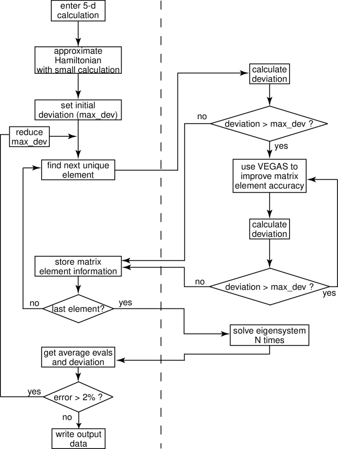
4 Saving Data

Saving basic data like the Hamiltonian and its error can be very useful because output can be rapidly regenerated or generated in a different format if needed. However there is much more important data that can be saved. The most cpu-expensive data generated while running this program is the statistical information generated by VEGAS for each integral.

In its basic form VEGAS only saves the information for the one integral it is calculating, and discards that information when it moves on to the next integral. The problem is that the same integral may need to be calculated more accurately in a later iteration, thus the integration would have to start from the beginning. Although saving the VEGAS information for each matrix element uses a lot of storage (30 integers, 1649 double precision), it is important to save all of it. If there is not enough memory available, the algorithm uses a scratch file to store the VEGAS information for the entire matrix. During most of a new calculation ($\approx 70-90\%$), there is little slowdown from disk access.

Despite the performance gain in modern computers, they are still subject to crashes. Also, if the code is running in parallel on many different computers, the chance of the code stalling due to a single computer failure increases. This problem can be remedied in a straightforward manner by occasionally saving the VEGAS information from memory to a file which can later be read in for code restart.

One final benefit of saving data, in particular the data for the five-dimensional integrals, is that the coupling is an overall factor multiplying all five-dimensional integrals. If the parameters vary only in the coupling from a previous run, the old matrix element estimates can be used as a starting point, which speeds searches through our parameter space.

5 Parallelizing The Algorithm

We first define the nomenclature we use when discussing the parallelized algorithm. The Message Passing Interface (MPI) uses one dispatcher process and several worker processes. In this algorithm the dispatcher is the organizer. It sends jobs for the workers to do and receives their results. In addition the dispatcher process does not use a lot of computer cycles and therefore does not require its own processor. There is an important distinction between processes and processors. The processor(s) is(are) the computer’s physical cpu(s), whereas the processes are simply jobs running on the machine. For example, on a particular machine, we typically run four processes on two processors. One process is the dispatcher and the remaining three are all workers.

There are many different ways this problem can be parallelized. For example, the matrix can be divided equally between the processors, each responsible for one submatrix. Another method is to let each process always work independently, moving from element to element until the desired error in the eigenvalues is reached. These two methods are examples of something that is too simple, and too complex, respectively. The first method assumes that each section of the matrix is equally important. However, the far off-diagonal elements are very small and calculating them to within more than an order of magnitude is often unnecessary. The second approach requires a very complicated method of tracking which process is working on which matrix element, trying to reach a particular deviation. Also it is not clear that this method would be efficient since only a handful of matrix elements are very important, and they take a lot of time to calculate to sufficient accuracy.

The philosophy we use in parallelizing the program is one of efficient simplicity. The method is simple because the calculation is broken up into steps and because no process continues to the next step until all other processes are ready to proceed. Efficiency is achieved by having processes that have finished help the processes that are still working.

Although the entire code is parallelized, we only discuss two sections in detail. The first is the parallelization of the error calculation and the second is the parallelization of the 5-d integral calculation. At the end of each iteration (reducing the deviation in the five-dimensional integrals) the error in the eigenvalues needs to be calculated. However, particularly for large matrices, this calculation can take a long time because it requires the complete eigensystem analysis. If only the dispatcher is used to do the error calculation, it may take several minutes, leaving all of the worker processes idle. The error calculation is parallelized by having each worker process generate an equal number of eigenvalue sets, then sending the results to the dispatcher, who then determines the averages and standard deviations.

The part of the calculation that benefits the most from parallel processing is the calculation of the five-dimensional integral contribution to each matrix element. Each matrix element can be calculated independently so there is almost no overhead due to communication between processes. A worker is given an assignment from the dispatcher. It then calculates it and returns the result, the process repeats with a new assignment, and an updated Hamiltonian. Figure 1, the simple algorithm, also shows which part of the flow is executed by the dispatcher process (left of dotted line) and the worker processes (right of dotted line). The only time this is not true is at the end of each iteration. Once all of the matrix elements have been assigned, as individual worker processes finish, the dispatcher directs them to help another worker process complete its assignment. The implementation of this “helping” algorithm is the first important and difficult addition to the parallelized algorithm.

If there is only one matrix element that requires a long time to calculate, then as the other workers finish, they sit idle waiting for the last element to be determined. This is a major drawback of the simple parallelization (independent matrix elements) since, except at the end of each iteration, the program can efficiently run using many processes. Thus, all but one process can be sitting idle while the last one continues to work. This can be remedied by having the dispatcher keep track of who is working and who is available to help. This increases the communication between the dispatcher and the worker at the time of assignment. The worker must be notified if it will be helping another process, or if it will get help, and who will be helping it. When the worker is finished it must let the dispatcher know if it was helping or getting help, etc. Figure 2 shows the flowchart for a worker process with the option to help other processes.

Helping Algorithm For a Worker Process

Figure 2: Flowchart for a worker process during the five-dimensional calculation, including the steps to help other processes. The double-lined arrows represent communication to and from the dispatcher.

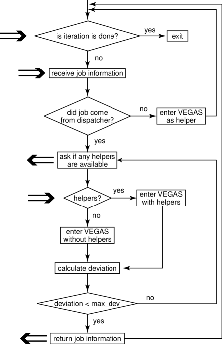
The last complication that requires additional communication between processes is saving VEGAS information. Not only should the VEGAS information be saved for the completed matrix elements, it should also be saved for calculations in progress. Otherwise, information from an integral that has consumed hours of cpu time might be lost. Thus the worker may also send updated VEGAS information, without sending a result. It is non-trivial to work out the communication between the worker and dispatcher process to allow for a wide range of information transfer.

6 Parallelized VEGAS

The parallelization of the numerical integrator is done in an attempt to limit the total number of communications between the worker in charge of a particular integral, and the processes helping it. Also, we do not want to get into the details of the adaptive nature of the integrator but do want a simple way of speeding the convergence of the integral.

The worker calls VEGAS with, among other things, the number of points to use and the number of iterations to attempt. After the desired number of iterations is completed, the routine statistically combines each of the iterations to get the result and its uncertainty. Thus, it is very straightforward to include information from the helper routines as extra iterations in the main worker.

The information that is lost using this method is that which helps refine the grid to make VEGAS an adaptive integrator. However, according to the documentation [41], the grid does not get significantly refined after a few iterations of a small number of points. Thus discarding the grid information should be unimportant.

Chapter 8 Results

In this Chapter we present our fully relativistic results for the meson mass spectrum. The results are presented along with experimental data [42] and predictions from a light-front calculation using a similar renormalization method with a nonrelativistic reduction [3, 4].

We first present important information about the experimental results we use. Our results begin with a brief description of the steps required to calculate the meson spectrum followed by two applications. We apply the method to the $b\bar{b}$ system as a check of the theory to verify that it agrees with nonrelativistic results and the $c\bar{c}$ system is investigated in detail. Finally, we show the spin-averaged meson probability densities defined in Eq. (72) to show what type of wavefunctions are produced.

1 Experimental Results

Heavy quarkonia states can be produced by colliding electrons and positrons. As the center-of-mass energy is changed, an increase in scattering events signals the existence of a resonance. The resonance is associated with a particle being created and then decaying into other particles. The mass of the initial particle is determined simply by finding the center-of-mass energy at which the resonance occurs. Daughter particle masses are determined by subtracting the energy of emitted photons or pions from the parent particle. Identifying the particles generated in a detector is not simple. One must infer the quantum numbers by knowing the quantum numbers of the beam and the daughter particles that are actually detected.

Although particle accelerators have produced a large amount of data that has been analyzed to give a plethora of information on spectroscopy of systems and transitions between particles, not all theoretically predicted particles have been seen. This fact is important when comparing new theoretical results to experimental data.

The charmonium system contains two (1S) states, the $J/\psi$ and the $\eta_{c}$. The $\eta_{c}$ is not directly produced in colliding $e^{+}e^{-}$ experiments but it is observed through transitions from the $J/\psi$ and other heavier states. The bottomonium system is also expected to have two (1S) states but the $\eta_{b}$ has not been seen experimentally because the transition from the $\Upsilon$ is greatly suppressed relative to the $J/\psi\rightarrow\gamma\eta_{c}$ because of the different quark masses, charges and photon energies.

2 Procedure

It should first be noted that there is no simple way to guarantee correct state identification when performing this calculation because, for instance, the spin operator is dynamic on the light-front as is equal-time parity. To simplify state identification, the quantum numbers we use for each data set include the z-component of the total spin ($j$) and charge conjugation (C). The drawback is that there are fewer low-lying states associated with each set of quantum numbers. For instance, the lowest five $b\bar{b}$ states contain two with negative charge conjugation ($n=0$ and $n=4$), and three with positive charge conjugation ($n=1,2,3$). We must use the $\mathrm{C}=+$ states to try to determine the mass ratios because we need at least two ratios to fix $m$ and $\alpha$.

There are two fundamental QCD parameters that need to be fixed, and the scale (cutoff) needs to be determined. The calculation produces eigenvalues of the renormalized invariant-mass operator, ${\cal M}^{2}(m_{{}_{\Lambda}},\Lambda)$. These eigenvalues are used to determine the fundamental QCD parameters and the cutoff. The steps to determine these values are described next.

Eigenvalues are generated for a set of $\alpha$ and $\frac{m}{\Lambda}$. If the renormalization was entirely non-perturbative and the Hamiltonian was calculated to all orders, the spectrum would be independent of the cutoff; however, we expect some cutoff dependence because we renormalize perturbatively and keep only two partons in our states. The renormalization is most trustworthy where there is little cutoff dependence.

The first step in finding the correct value of $\alpha$ and $\frac{m}{\Lambda}$ is to determine the cutoff by fixing one mass using the relation:

$$\Lambda^{2}=\frac{m^{2}_{measured}}{\langle i|{\cal M}^{2}(\Lambda)|i\rangle},$$ (1)

where $m^{2}_{measured}$ is taken from [42] and $i$ refers to the state used to fix the cutoff. Next the rest of the meson spectrum can be calculated using this cutoff:

$$m^{2(j)}_{calculated}=\Lambda^{2}\langle j|{\cal M}^{2}(\Lambda)|j\rangle,$$ (2)

where $j$ refers to the state being calculated.

Secondly we analyze the spectrum for a range of $\alpha$ and $\frac{m}{\Lambda}$ to find the values that give the correct values for the lowest and second lowest mass states above the state we fix. Finding which values of $\alpha$ and $\frac{m}{\Lambda}$ correctly determine these two observables gives us our best values of $\alpha$ and $\frac{m}{\Lambda}$ .

3 Convergence Testing

We must be certain we are using an adequate number of basis functions when taking final data. We verify our results have converged for various values of $\frac{m}{\Lambda}$ with $\alpha=\frac{1}{2}.$ We reiterate that it is not necessary for the ground state eigenvalue to decrease as each additional function is added since the previous functions are shifted .

Increasing the order of the B-splines ($m$ in B-spline notation) beyond third order does not improve convergence, but increases the number of nonzero matrix elements. Therefore all B-splines we use are third order. Figures 1 through 9 show the convergence of the lowest three states for $\frac{m}{\Lambda}=.2$, $.8$, and $1.5$ as we increase the number of longitudinal and transverse states. The number of B-splines in the longitudinal direction is:

$$k_{1}+m+1-2=k_{1}+2,$$ (3)

where two states are not used because they have the incorrect behavior as $x\rightarrow 0,1$. We pair the splines into symmetric and antisymmetric functions under particle exchange (see Sec. 1). Thus the total number of splines in the longitudinal direction is:

$$\mathrm{N}_{l}=\frac{k_{1}}{2}+1.$$ (4)

Similarly the number of B-splines in the transverse direction is:

$$\mathrm{N}_{t}=k_{2}+m+1-3=k_{2}+1,$$ (5)

where three states are not used to ensure finite kinetic energy due to small x singularities.

Figure 1: Convergence of the ground state for $\frac{m}{\Lambda}$ $=.2$ and $\alpha=.5$.

Figure 2: Convergence of the first exited state for $\frac{m}{\Lambda}$ $=.2$ and $\alpha=.5$.

Figure 3: Convergence of the second excited state for $\frac{m}{\Lambda}$ $=.2$ and $\alpha=.5$.

Figure 4: Convergence of the ground state for $\frac{m}{\Lambda}$ $=.8$ and $\alpha=.5$.

Figure 5: Convergence of the first exited state for $\frac{m}{\Lambda}$ $=.8$ and $\alpha=.5$.

Figure 6: Convergence of the second excited state for $\frac{m}{\Lambda}$ $=.8$ and $\alpha=.5$.

Figure 7: Convergence of the ground state for $\frac{m}{\Lambda}$ $=1.5$ and $\alpha=.5$.

Figure 8: Convergence of the first exited state for $\frac{m}{\Lambda}$ $=1.5$ and $\alpha=.5$.

Figure 9: Convergence of the second excited state for $\frac{m}{\Lambda}$ $=1.5$ and $\alpha=.5$.

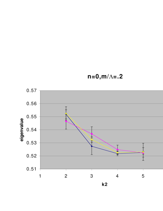
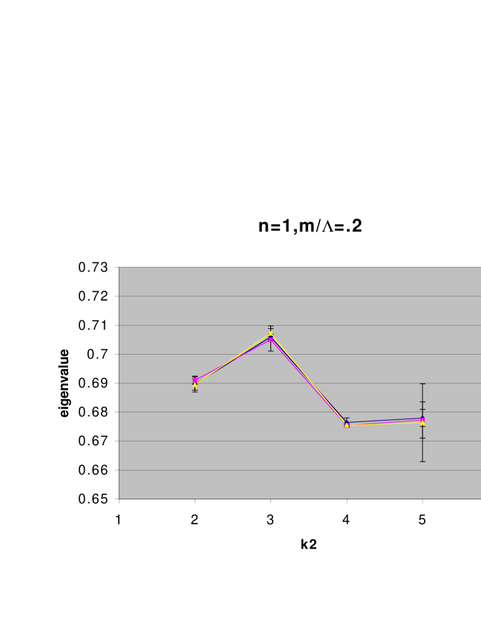
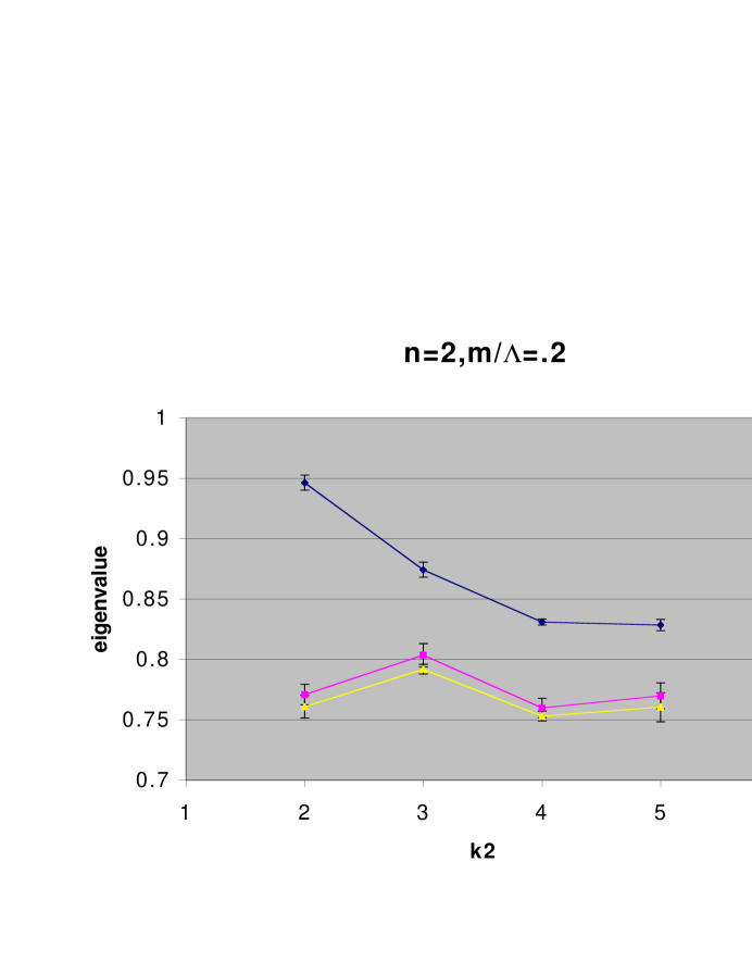
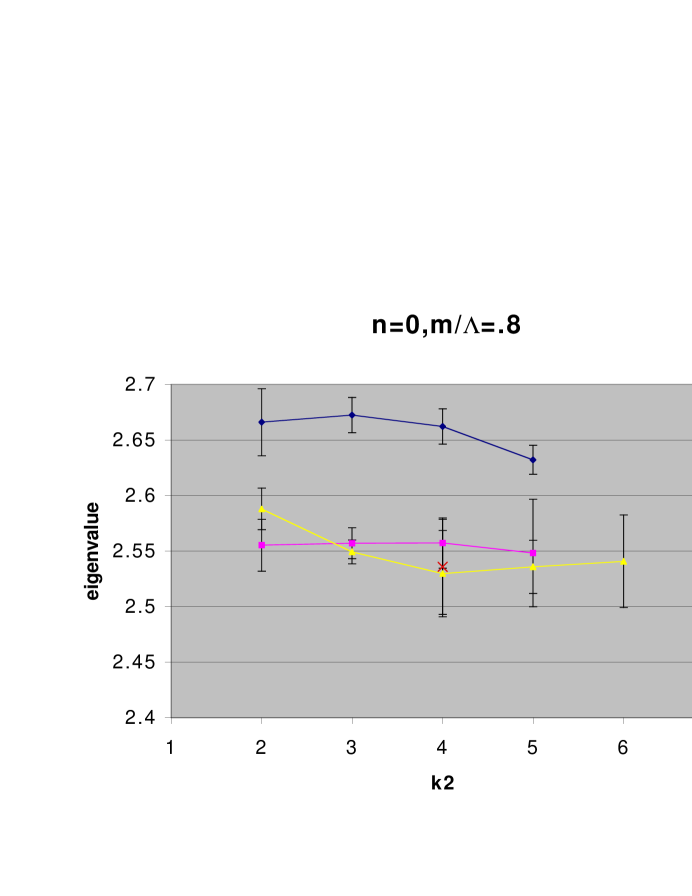
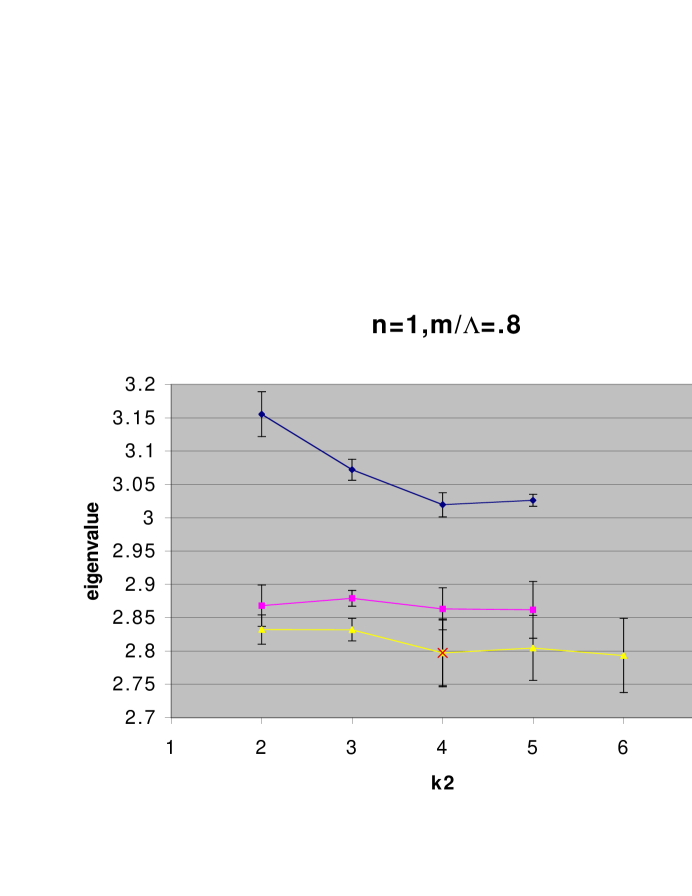
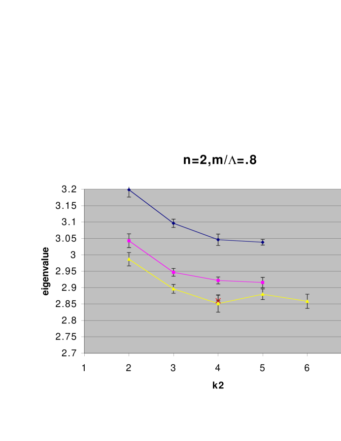
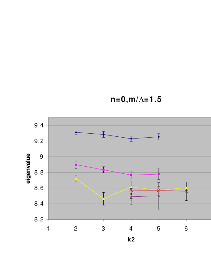
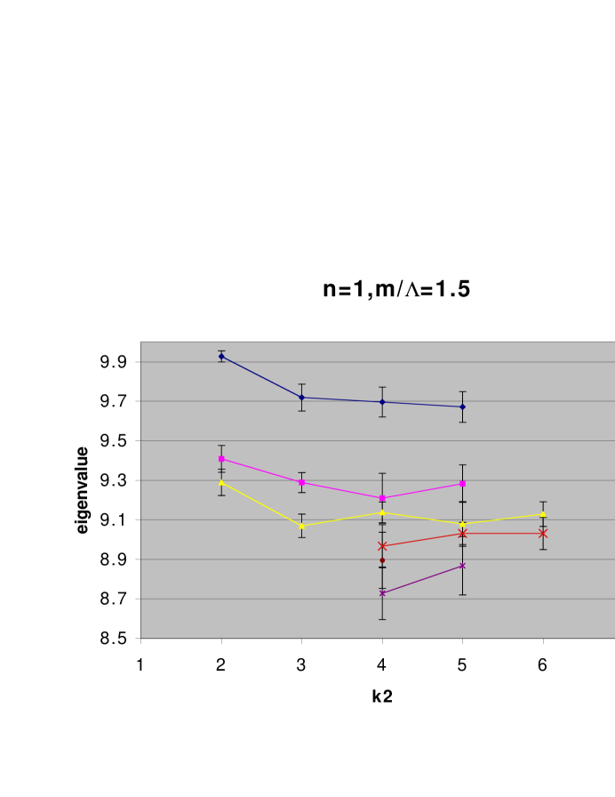
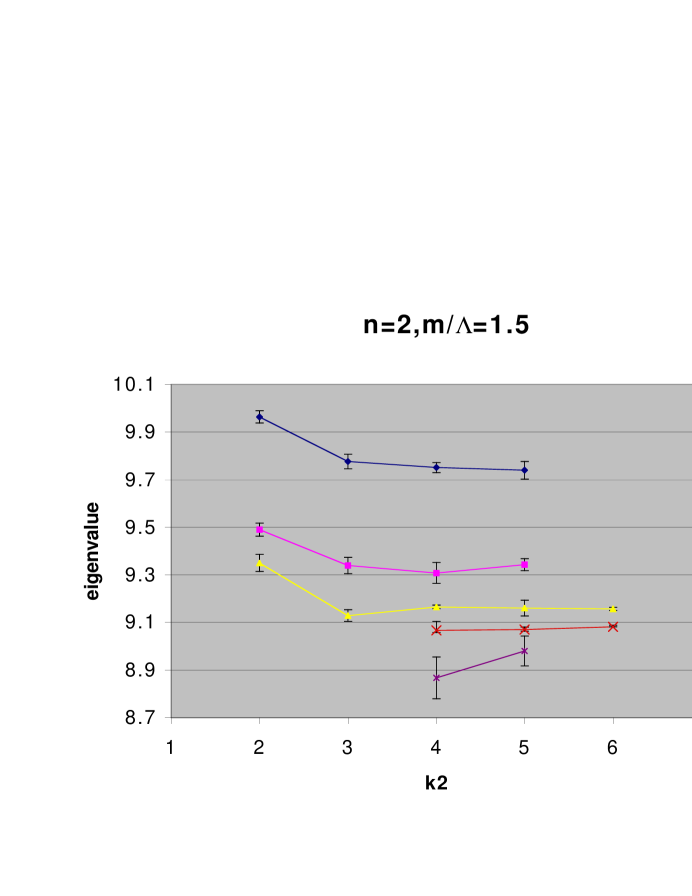
As $\frac{m}{\Lambda}$ increases a larger number of longitudinal states are needed for the eigenvalues to converge. Although we could have used fewer basis functions for smaller values of $\frac{m}{\Lambda}$ , all of our calculations use $k_{1}=8$ and $k_{2}=5$. Using equations (4), (5), and noting that we have four spin states, the number of basis states we use is:

$$4\times N_{l}\times N_{t}=4\times 5\times 6=120.$$ (6)

Since the Hamiltonian is Hermitian, at most 7260 of the 14400 matrix elements are unique. Since not all of the B-splines spatially overlap all of the other B-splines, there are 1680 elements that are zero. For our choice of $k_{1}$ and $k_{2}$ we have reduced the number of elements that need to be calculated by $23\%$.

4 Error Estimation

There are three sources of errors in our meson spectra. Since we do not use an infinite number of basis functions we can not exactly determine the eigenvalues of our Hamiltonian. Based on our convergence testing, we can choose the smallest number of basis functions that produce converged eigenvalues to within two percent. These eigenvalues are of the Hamiltonian (IMO), so a two percent error in the eigenvalues will produce approximately a one percent error in the masses.

The second source of errors is statistical. Each matrix element is calculated by Monte-Carlo integration which suffers from statistical uncertainty. We calculate the error in the eigenvalues by allowing each matrix element to vary randomly within its gaussian distribution. This is done many times to generate a large number of eigenvalue sets that are used to calculate the average eigenvalue and the errors in the eigenvalues. The largest error allowed in any eigenvalue is two percent, giving a one percent error in the masses.

The final and most significant source of error is in our approximation of the theory: limiting the approximate states to a quark-antiquark pair and truncating the Hamiltonian at second order in the coupling. We cannot reliably estimate the error produced by our approximation to the real state without first solving the meson spectrum with $|q\bar{q}g\rangle$ states. We can estimate the error from approximating the Hamiltonian.

Our Hamiltonian contains a contribution from the kinetic energy and second-order interactions, so we should expect errors of order $g^{4}$ ($\alpha^{2}$); however, for the heaviest mesons the errors in the masses should be very small because they are dominated by the kinetic energy. We can write

$${\cal H}(1+\delta)=\mathrm{KE}+V(1+\epsilon)$$ (7)

where $\delta$ is the fractional error in the Hamiltonian and $\epsilon$ is the fractional error in the interactions ($\frac{g^{4}}{g^{2}}=g^{2}\propto\alpha$). However, what we actually solved is

$${\cal H}=\mathrm{KE}+V.$$ (8)

We can now solve for the fractional error in the binding energy by considering the expectation values of ${\cal H}$ and KE:

$$\delta=\epsilon\frac{\langle{\cal H}\rangle-\langle\mathrm{KE}\rangle}{\langle{\cal H}\rangle}\propto\alpha\frac{\langle{\cal H}\rangle-\langle\mathrm{KE}\rangle}{\langle{\cal H}\rangle},$$ (9)

where we used the fact that the corrections to the interactions are ${\cal O}(\alpha)$. This means the error in the eigenvalues is roughly $\alpha$ times the fraction of the eigenvalue that comes from the interaction.

5 $b\bar{b}$ Spectrum

We calculate the $b\bar{b}$ spectrum to verify that our method gives similar results to [3, 4], which uses nonrelativistic reduction (NR Reduction). The splittings in the $b\bar{b}$ system are so small that our method can not determine them in a reasonable amount of time. However the comparison is useful to make sure that we get similar results for the quark mass, cutoff and meson masses. With the small splittings, our method also has little predictive power for this system.

We use the values $\alpha=.4$ and $\frac{m}{\Lambda}=1.38$ from [3] and determine the cutoff to be $3.6$ GeV by fixing the mass of $\chi_{b_{0}}$ (the lowest $\mathrm{C}=+$ state) to data. Table 1 shows our results (Fully Relativistic) along with the experimental results as well as those calculated using NR Reduction. $3.5\%$ of mass of the $\chi_{b_{0}}$ is due to interactions. Thus we believe the errors in our bottomonium spectrum due to our approximate Hamiltonian to be about $1.4\%$. Our spectrum agrees with the other results within errors. This method passes the simplest test.

State	Experimental	NR Reduction	Fully Relativistic
$\Upsilon_{a}$	$9.460$	$9.4$	$9.64\pm.1\pm.1\pm.14$
$\chi_{b_{0}}$	$9.860$	$9.9$	N/A
$\chi_{b_{1}}$	$9.893$	$9.9$	$9.87\pm.1\pm.1\pm.14$
$\chi_{b_{2}}$	$9.913$	$9.9$	$9.88\pm.1\pm.1\pm.14$
$\Upsilon_{b}$	$10.023$	N/A	$9.86\pm.1\pm.1\pm.14$

Table 1: Bottomonium masses in GeV from experimental results, nonrelativistic reduction and our fully relativistic calculation. The NR Reduction and Fully Relativistic calculations use $\alpha=.4$ and $m=4.9$ GeV. The errors given for the relativistic calculation are from using a finite number of basis states, statistics and our second-order approximation to the Hamiltonian.

The wavefunctions for the $\Upsilon_{a}$, $\chi_{b_{0}}$, $\chi_{b_{1}}$, and $\chi_{b_{2}}$, with $\alpha=.4$ and $j=0$ are plotted in figures 10, 11, 12, and 13 respectively.

Figure 10: $\Upsilon_{a}$ wavefunction. $x$ is the longitudinal momentum fraction carried by one particle and $k$ is the relative transverse momentum in units of the cutoff.

Figure 11: $\chi_{b_{0}}$ wavefunction. $x$ is the longitudinal momentum fraction carried by one particle and $k$ is the relative transverse momentum in units of the cutoff.

Figure 12: $\chi_{b_{1}}$ wavefunction. $x$ is the longitudinal momentum fraction carried by one particle and $k$ is the relative transverse momentum in units of the cutoff.

Figure 13: $\chi_{b_{2}}$ wavefunction. $x$ is the longitudinal momentum fraction carried by one particle and $k$ is the relative transverse momentum in units of the cutoff.

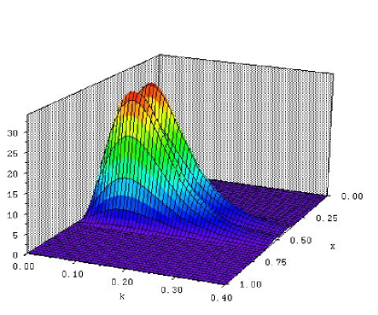
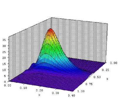
6 $c\bar{c}$ Spectrum

Our approximations may work best for the $c\bar{c}$ system. We find a good representation of the mass spectrum, but find unusual values for the coupling and cutoff. If we use the values of the coupling and $\frac{m}{\Lambda}$ from [4] we do not fit the spectrum within errors.

We first generate eigenvalues for $.1\leq\alpha\leq.9$ and $.1\leq\frac{m}{\Lambda}\leq 1$ for states with positive charge conjugation since only one of the five lightest states in the $c\bar{c}$ spectrum has negative charge conjugation. $\eta_{c}$ is used to determine the cutoff which is plotted (in MeV) against $\alpha$ and $\frac{m}{\Lambda}$ in Figure 14.

Figure 14: The cutoff (MeV) versus the coupling and the charm quark mass divided by the cutoff.

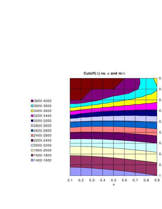
Using the corresponding value of $\Lambda$ for $\alpha$ and $\frac{m}{\Lambda}$ , we plot the mass of the first (n=1) and second (n=2) excited positive-charge-conjugation states in figures 15 and 16 respectively.

Figure 15: Mass of the first excited positive-charge-conjugation state, $\chi_{c_{0}}$ as a function of $\alpha$ and $\frac{m}{\Lambda}$ . The experimental value is 3417 MeV and each color band represents a mass range equal to two percent of the experimental mass.

Figure 16: Mass of the second excited positive-charge-conjugation state, $\chi_{c_{1}}$ as a function of $\alpha$ and $\frac{m}{\Lambda}$ . The experimental value is 3510 MeV and each color band represents a mass range equal to two percent of the experimental mass.

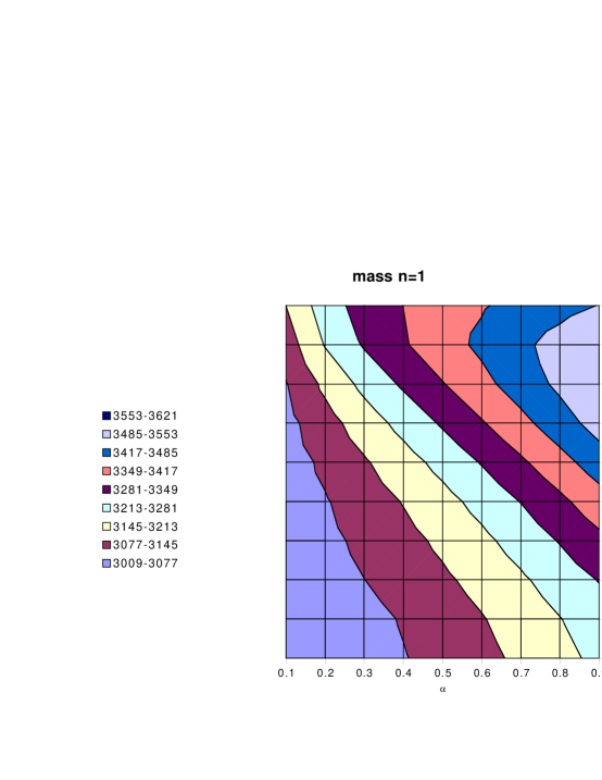
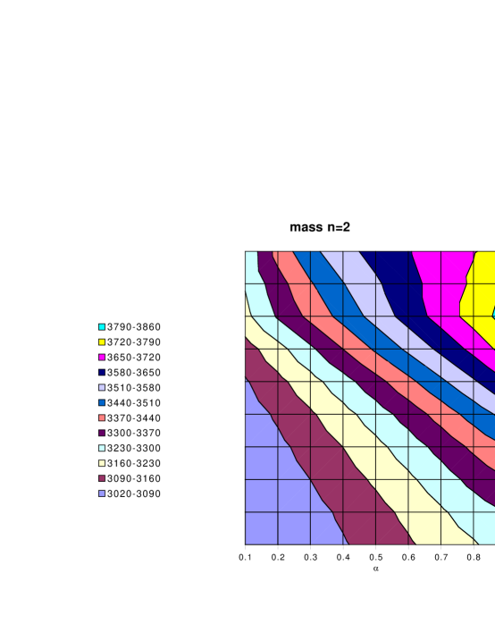
We find the values $\alpha$ and $\frac{m}{\Lambda}$ that correctly produce the ratios of the first and second exited states by finding the region where the mass of the first and second excited states are predicted to within two percent. Figure 17 shows where both masses are predicted within the error.

Figure 17: This figure displays the success for choices of $\alpha$ and $\frac{m}{\Lambda}$ at predicting the first and second excited state masses. We define a correct prediction to be within two percent of the actual value. The value is zero (purple) if neither mass is correctly determined, one (red) if one mass is correctly predicted and two (yellow) if both are correct.

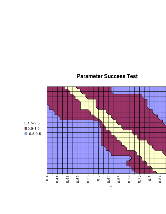
Unfortunately fixing these two masses is not sufficient to determine $\alpha$ and $\frac{m}{\Lambda}$ because there is a range of $\alpha$ and $\frac{m}{\Lambda}$ that correctly predict the spectrum. Also as $\frac{m}{\Lambda}$ is lowered the eigenvalues become smaller, increasing the cutoff. All of the combinations of $\alpha$ and $\frac{m}{\Lambda}$ that successfully predict the spectrum produce a cutoff and/or coupling that is too large to be consistent with our ${\cal O}(g^{2})$ approximation. If we consider $\alpha=\frac{1}{2}$ and $\frac{m}{\Lambda}$ $=.28$, we get a cutoff of $3.8$ GeV and the mass of the charm quark equal to $1.05$ GeV. It is clear the errors generated by our approximations are too large to successfully predict the charmonium spectrum.

If we use $\alpha=.5$ and $\frac{m}{\Lambda}$ $=.88$ from [4] we find the spectrum in Table 2 and determine the cutoff to be $1.7$ GeV, and the charm quark mass to be $1.5$ GeV. $5\%$ of the $\eta_{c}$ mass is due to interactions, making the error from the approximate Hamiltonian in our spectrum about $2.5\%$.

State	Experimental	NR Reduction	Fully Relativistic
$\eta_{c}$	$2.9798$	$3.0$	N/A
$J/\psi$	$3.097$	$3.0$	$2.981\pm 0.03\pm 0.03\pm 0.075$
$\chi_{c_{0}}$	$3.415$	3.5	$3.114\pm 0.03\pm 0.03\pm 0.078$
$\chi_{c_{1}}$	$3.510$	$3.5$	$3.142\pm 0.03\pm 0.03\pm 0.079$
$\chi_{c_{2}}$	$3.556$	$3.5$	$3.145\pm 0.03\pm 0.03\pm 0.079$

Table 2: Charmonium masses in GeV from experimental results, nonrelativistic reduction and fully relativistic calculations with $\alpha=.5$ and $\frac{m}{\Lambda}$ $=.88$. The errors given for the Fully Relativistic calculation are from using a finite number of basis states, statistics and our second-order approximation to the Hamiltonian.

The spin-averaged probability densities for the $\eta_{c}$, $J/\psi$, $\chi_{c_{0}}$ and $\chi_{c_{1}}$ with $\alpha=.5$ and $\frac{m}{\Lambda}$ $=.88$ are shown in figures 18 through 21, respectively.

Figure 18: $\eta_{c}$ wavefunction. $x$ is the longitudinal momentum fraction carried by one particle and $k$ is the relative transverse momentum in units of the cutoff.

Figure 19: $J/\psi$ wavefunction. $x$ is the longitudinal momentum fraction carried by one particle and $k$ is the relative transverse momentum in units of the cutoff.

Figure 20: $\chi_{c_{0}}$ wavefunction. $x$ is the longitudinal momentum fraction carried by one particle and $k$ is the relative transverse momentum in units of the cutoff.

Figure 21: $\chi_{c_{1}}$ wavefunction. $x$ is the longitudinal momentum fraction carried by one particle and $k$ is the relative transverse momentum in units of the cutoff.

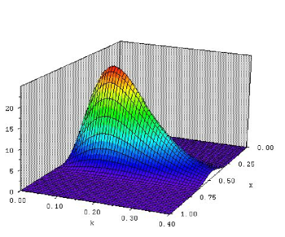
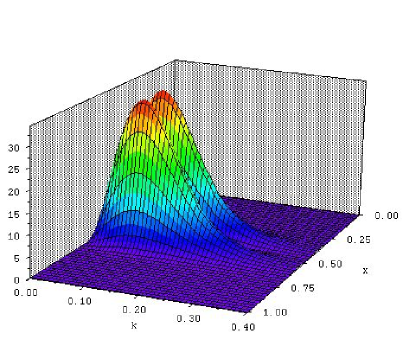
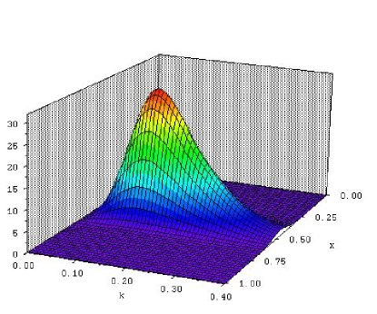
Chapter 9 Conclusions and Future

The method we use to regulate and renormalize the light-front QCD Hamiltonian does not remove any physics, add extra parameters or fundamentally limit itself to particular problems (like heavy quark systems). The renormalized, second-order, light-front Hamiltonian is reasonably successful at determining the glueball spectrum. This same approximation is much less successful at determining the heavy meson spectra.

The success of the glueball calculation shows our method can be successful. It is clear that to more successfully determine (with predictive power) the heavy meson spectra we must either calculate the renormalized Hamiltonian to higher order in the strong coupling and/or allow for more complicated external states ($q\bar{q}g$). In addition to these improvements using basis functions that are more sharply peaked should improve the accuracy of the heaviest meson system ($b\bar{b}$) where the difference in the masses are fractions of a percent.

We determined the light-front Hamiltonian to second order in the strong coupling while approximating the real states as a quark-antiquark pair. The results from the glueball and meson mass calculations show our method can reproduce experimental results with varying degrees of success. The renormalized Hamiltonian we determined is the building block of higher order calculations and will be a necessary part of future calculations.

It is unclear if B-splines are an efficient basis to approximate the real states. They reproduced the glueball spectrum with fewer basis functions than an earlier calculation but appear inefficient at representing the sharply peaked heavy meson wave functions. Although the full flexibility of the B-splines was not explored, it is likely more efficient to use basis functions better tailored to the problem at hand.

The analytic calculation of the renormalized Hamiltonian requires a large time investment and great care. However the analytic result is not very useful without an effective and efficient method to numerically calculate the integrals the analytic calculation yields. We developed an algorithm to calculate these integrals without wasting time calculating any matrix element more accurately than needed. We also generalized the algorithm to run on a single processor or in a parallel processor environment, including clusters of desktop machines. This is a significant development because the algorithm is independent of the details of the integrand so higher order analytic calculations can utilize it with very little change.

We successfully added to the systematic determination of the renormalized light-front Hamiltonian by including masses. We explored the effectiveness of B-spline basis functions and developed an algorithm for calculating the renormalized Hamiltonian matrix.

Chapter 10 Light-Front Conventions

In this Appendix we list the light-front conventions used in this dissertation. For a more general introduction see the light-front review by A. Harindranath [43].

Appendix 10.A Coordinates

$$\begin{array}[]{ll}x^{\pm}=x^{0}\pm x^{3}&x\cdot y=\frac{1}{2}x^{+}y^{-}+\frac{1}{2}x^{-}y^{+}-x^{i}_{\bot}y^{i}_{\bot}\\ \partial^{\pm}=2\frac{\partial}{\partial x^{\mp}}&\partial\cdot x=\frac{1}{2}\partial^{+}x^{-}+\frac{1}{2}\partial^{-}x^{+}-\partial^{i}_{\bot}x^{i}_{\bot}\\ \partial^{i}_{\bot}=-\frac{\partial}{\partial x^{i}_{\bot}}\end{array}$$

$$\begin{array}[]{lll}x^{\mu}=\left(\begin{array}[]{c}x^{+}\\ x^{-}\\ x^{1}\\ x^{2}\end{array}\right)&\hskip 14.22636ptg^{\mu\nu}=\left(\begin{array}[]{rrrr}0&2&0&0\\ 2&0&0&0\\ 0&0&-1&0\\ 0&0&0&-1\end{array}\right)&\hskip 14.22636ptg_{\mu\nu}=\left(\begin{array}[]{rrrr}0&\frac{1}{2}&0&0\\ \frac{1}{2}&0&0&0\\ 0&0&-1&0\\ 0&0&0&-1\end{array}\right)\end{array}$$ (17)

Appendix 10.B Gamma Matrices

$$\begin{array}[]{lll}\gamma^{+}=\left(\begin{array}[]{cc}0&0\\ 2i&0\end{array}\right)&\hskip 14.22636pt\gamma^{-}=\left(\begin{array}[]{cc}0&-2i\\ 0&0\end{array}\right)&\hskip 14.22636pt\gamma^{0}=\left(\begin{array}[]{cc}0&-i\\ i&0\end{array}\right)\\ \gamma^{5}=\left(\begin{array}[]{cc}\sigma^{3}&0\\ 0&-\sigma^{3}\end{array}\right)&\hskip 14.22636pt\gamma^{i}=\left(\begin{array}[]{cc}-i\sigma^{i}&0\\ 0&i\sigma^{i}\end{array}\right)&\hskip 14.22636pt\alpha^{i}_{\bot}=\left(\begin{array}[]{cc}0&\sigma^{i}_{\bot}\\ \sigma^{i}_{\bot}&0\end{array}\right)\end{array}$$ (32)

Appendix 10.C Pauli Matrices

$$\sigma^{1}=\left(\begin{array}[]{cc}0&1\\ 1&0\end{array}\right)\hskip 28.45274pt\sigma^{2}=\left(\begin{array}[]{cc}0&-i\\ i&0\end{array}\right)\hskip 28.45274pt\sigma^{3}=\left(\begin{array}[]{cc}1&0\\ 0&-1\end{array}\right)$$ (39)

Appendix 10.D Projection Operators

$$\Lambda_{\pm} = \frac{1}{2}\gamma^{0}\gamma^{\pm}$$

$$\Lambda_{+} = \frac{1}{2}\left(\begin{array}[]{rr}0&-i\\ i&0\end{array}\right)\left(\begin{array}[]{rr}0&0\\ 2i&0\end{array}\right)=\left(\begin{array}[]{rr}1&0\\ 0&0\end{array}\right)$$ (46)

$$\Lambda_{-} = \frac{1}{2}\left(\begin{array}[]{rr}0&-i\\ i&0\end{array}\right)\left(\begin{array}[]{rr}0&-2i\\ 0&0\end{array}\right)=\left(\begin{array}[]{rr}0&0\\ 0&1\end{array}\right)$$ (53)

Note:

$$\begin{array}[]{lll}\Lambda_{+}+\Lambda_{-}=1&\Lambda_{+}^{2}=\Lambda_{+}&\Lambda_{-}^{2}=\Lambda_{-}\\ \Lambda_{\pm}\Lambda_{\mp}=0&\gamma^{+}\gamma^{+}=\gamma^{-}\gamma^{-}=0&(\gamma^{\pm})^{\dagger}=\gamma^{\mp}\\ \Lambda_{\pm}^{\dagger}=\Lambda_{\pm}&\gamma^{0}\gamma^{\pm}=\gamma^{\mp}\gamma^{0}&\gamma^{i}_{\bot}\gamma^{\pm}=-\gamma^{\pm}\gamma^{i}_{\bot}\\ \gamma^{\mp}\gamma^{\pm}=4\Lambda_{\pm}&\alpha^{i}_{\bot}\Lambda_{\pm}=\Lambda_{\mp}\alpha^{i}_{\bot}&\gamma^{0}\Lambda_{\pm}=\Lambda_{\mp}\gamma^{0}\end{array}$$

Appendix 10.E Lagrangian

$${\cal L}_{\mathrm{QCD}}=-\frac{1}{4}F_{\mu\nu}^{c}F^{\mu\nu}_{c}+\bar{\psi}(iD/-m_{F})\psi,$$ (58)

where

$$F^{\mu\nu}_{c}=\partial^{\mu}A_{c}^{\nu}-\partial^{\nu}A_{c}^{\mu}-gA^{\mu}_{c_{1}}A^{\nu}_{c_{2}}f^{c_{1}c_{2}c}$$ (59)

and

$${\bf D}_{\mu}\psi=(\partial_{\mu}+igA^{a}_{\mu}{\bf T}_{a})\psi.$$ (60)

Greek indices are Lorentz indices, $c$’s are color indices, $\alpha$ is the color index, repeated indices are summed over, and the $f$’s are the SU($N_{c}$) structure constants. The ${\bf T}_{a}$’s are the $SU(3)$ Gell-Mann matrices which obey the commutation relation $\left[{\bf T}_{a},{\bf T}_{b}\right]=if_{abc}{\bf T}_{c}$ and are given by:

$$\begin{array}[]{llll}{\bf T}_{1}=\frac{1}{2}\left(\begin{array}[]{ccc}0&1&0\\ 1&0&0\\ 0&0&0\end{array}\right)&{\bf T}_{2}=\frac{1}{2}\left(\begin{array}[]{ccc}0&-i&0\\ i&0&0\\ 0&0&0\end{array}\right)&{\bf T}_{3}=\frac{1}{2}\left(\begin{array}[]{ccc}1&0&0\\ 0&-1&0\\ 0&0&0\end{array}\right)&{\bf T}_{4}=\frac{1}{2}\left(\begin{array}[]{ccc}0&0&1\\ 0&0&0\\ 1&0&0\end{array}\right)\\ {\bf T}_{5}=\frac{1}{2}\left(\begin{array}[]{ccc}0&0&-i\\ 0&0&0\\ i&0&0\end{array}\right)&{\bf T}_{6}=\frac{1}{2}\left(\begin{array}[]{ccc}0&0&0\\ 0&0&1\\ 0&1&0\end{array}\right)&{\bf T}_{7}=\frac{1}{2}\left(\begin{array}[]{ccc}0&0&0\\ 0&0&-i\\ 0&i&0\end{array}\right)&{\bf T}_{8}=\frac{1}{2}\left(\begin{array}[]{ccc}\frac{1}{\sqrt{3}}&0&0\\ 0&\frac{1}{\sqrt{3}}&0\\ 0&0&\frac{-2}{\sqrt{3}}\end{array}\right).\end{array}$$ (87)

Appendix 10.F The Gluon Field

The expansion of the transverse gluon field takes the form:

$$\vec{A}_{c\bot}(x^{-},\vec{x_{\bot}})=\int D_{i}\delta_{c,c_{i}}\left[a_{i}\vec{\epsilon}_{\bot s_{i}}e^{-ip_{i}\cdot x}+a^{\dagger}_{i}\vec{\epsilon}_{\bot s_{i}}^{\hskip 2.84544pt\ast}e^{ip_{i}\cdot x}\right]|_{x^{+}=0},$$ (88)

where

$$D_{i}=\sum_{c_{i}=1}^{N_{c}}\sum_{s_{i}=-1,1}\frac{d^{2}p_{i\bot}dp_{i}^{+}}{16\pi^{3}p_{i}^{+}}\theta(p_{i}^{+}-\epsilon{\cal P}^{+}),$$ (89)

${\cal P}$ is the four-momentum operator, $\epsilon$ is a positive infinitesimal, and

$$\vec{\epsilon}_{\bot s}=\frac{-1}{\sqrt{2}}(s,i).$$ (90)

The creation and annihilation operators follow the convention

$$a_{i}=a(p_{i},s_{i},c_{i}),$$ (91)

and have the commutation relations

$$[a_{i},a_{j}^{\dagger}]=16\pi^{3}p_{i}^{+}\delta^{(3)}(p_{i}-p_{j})\delta_{s_{i},s_{j}}\delta_{c_{i},c_{j}}$$ (92)

and

$$[a_{i},a_{j}]=[a_{i}^{\dagger},a_{j}^{\dagger}]=0,$$ (93)

where

$$\delta^{(3)}(p_{i}-p_{j})=\delta(p_{i}^{+}-p_{j}^{+})\delta^{(2)}(\vec{p}_{i\bot}-\vec{p}_{j\bot}).$$ (94)

The gluon field commutation relation is:

$$\left[A^{ic_{1}}_{\bot}(x),\partial^{+}A^{jc_{2}}_{\bot}(y)\right]_{x^{+}=y^{+}=0}=i\delta^{ij}\delta_{c_{1}c_{2}}\delta^{3}(x-y).$$ (95)

Appendix 10.G Gluon Polarization Vector

The gluon polarization vector is

$$\epsilon^{+}=0,\hskip 14.22636pt\epsilon^{-}=\frac{2{\bf q}_{\bot}\cdot\epsilon_{\bot}}{q^{+}},$$ (96)

and

$$\sum_{\lambda}\epsilon^{\mu}_{\bot}(\lambda)\epsilon^{\ast\hskip 1.42271pt\nu}_{\bot}(\lambda)=-g^{\mu\nu}_{\bot},$$ (97)

so that

$$\sum_{\lambda}\epsilon^{\mu}(\lambda)\epsilon^{\ast\hskip 1.42271pt\nu}(\lambda)=g^{\mu\nu}_{\bot}+\frac{1}{q^{+}}\left(\eta^{\mu}q^{\nu}_{\bot}+\eta^{\nu}q^{\mu}_{\bot}\right)+\frac{{\bf q}_{\bot}^{2}}{(q^{+})^{2}}\eta^{\mu}\eta^{\nu},$$ (98)

where $\eta^{+}=\eta^{1}=\eta^{2}=0$ and $\eta^{-}=2$. Also

$$\vec{\epsilon}_{\bot\lambda}\cdot\vec{\epsilon}^{\hskip 2.84544pt\ast}_{\bot\lambda^{\prime}}=\delta_{\lambda\lambda^{\prime}}\hskip 28.45274pt\vec{\epsilon}_{\bot\lambda}\cdot\vec{\epsilon}_{\bot\lambda^{\prime}}=-\delta_{\lambda\lambda^{\prime}}.$$ (99)

We can write them out:

$$\epsilon^{\mu}_{\bot 1}=\left(\begin{array}[]{c}0\\ 0\\ -\frac{1}{\sqrt{2}}\\ -\frac{i}{\sqrt{2}}\end{array}\right)\hskip 56.9055pt\epsilon^{\mu}_{\bot-1}=\left(\begin{array}[]{c}0\\ 0\\ \frac{1}{\sqrt{2}}\\ -\frac{i}{\sqrt{2}}\end{array}\right).$$ (108)

We also find:

$$\sigma_{\bot}\cdot\epsilon^{\bot}_{-1}=-\sigma_{\bot}\cdot\epsilon^{\bot\ast}_{1}=\sqrt{2}\left(\begin{array}[]{cc}0&0\\ 1&0\end{array}\right)\hskip 14.22636pt\sigma_{\bot}\cdot\epsilon^{\bot\ast}_{-1}=-\sigma_{\bot}\cdot\epsilon_{1}^{\bot}=\sqrt{2}\left(\begin{array}[]{cc}0&1\\ 0&0\end{array}\right)$$ (113)

Appendix 10.H The Fermion Field

The dynamical fermion degree of freedom is $\psi_{+}$ and can be expanded in terms of plane wave creation and annihilation operators at $x^{+}=0$,

$$\psi_{+}^{c}\left(x^{-},\vec{x}_{\bot}\right)=\int D_{1}\delta_{c,c1}\left[b_{1}u_{+}(k,\sigma)e^{-ik\cdot x}+d^{\dagger}_{1}v_{+}(k,\sigma)e^{ik\cdot x}\right],$$ (114)

$$\psi_{+}^{c\dagger}\left(x^{-},\vec{x}_{\bot}\right)=\int D_{1}\delta_{c,c1}\left[b^{\dagger}_{1}u_{+}^{\dagger}(k,\sigma)e^{ik\cdot x}+d_{1}v_{+}^{\dagger}(k,\sigma)e^{-ik\cdot x}\right],$$ (115)

where the creation and annihilation operators are labeled the same as in Section 10.F. The field operators satisfy

$$\left\{\psi^{c_{1}}_{+}(x),\psi^{c_{2}\hskip 1.42271pt\dagger}_{+}(y)\right\}_{x^{+}=y^{+}=0}=\Lambda_{+}\delta_{c_{1},c_{2}}\delta^{3}(x-y),$$ (116)

and the creation and annihilation operators satisfy:

$$\left\{b_{i},b^{\dagger}_{j}\right\}=\left\{d_{i},d^{\dagger}_{j}\right\}=16\pi^{3}p^{+}\delta_{c_{i},c_{j}}\delta_{s_{i},s_{j}}\delta^{3}(p_{i}-p_{j}).$$ (117)

Appendix 10.I Dirac Spinors

The dirac spinors $u(p,\sigma)$ and $v(p,\sigma)$ satisfy

$$\left(p/-m\right)u(p,\sigma)=0,\hskip 14.22636pt\left(p/+m\right)v(p,\sigma)=0,$$ (118)

and

$$\bar{u}(p,\sigma)u(p,\sigma^{\prime}) = -\bar{v}(p,\sigma)v(p,\sigma^{\prime})=2m\delta_{\sigma\sigma^{\prime}},$$ (119)

$$\bar{u}(p,\sigma)\gamma^{\mu}u(p,\sigma^{\prime}) = \bar{v}(p,\sigma)\gamma^{\mu}v(p,\sigma^{\prime})=2p^{\mu}\delta_{\sigma\sigma^{\prime}},$$ (120)

$$\sum_{\sigma=\pm\frac{1}{2}}u(p,\sigma)\bar{u}(p,\sigma)=p/+m,\hskip 14.22636pt\sum_{\sigma=\pm\frac{1}{2}}v(p,\sigma)\bar{v}(p,\sigma)=p/-m.$$ (121)

We use the normalizations:

$$u^{\dagger}_{+k\lambda^{\prime}}\hskip 2.84544ptu_{+k\lambda}=v^{\dagger}_{+k\lambda^{\prime}}\hskip 2.84544ptv_{+k\lambda}=k^{+}\delta_{\lambda,\lambda^{\prime}}.$$ (122)

We can define:

$$u_{+k\lambda}\equiv\sqrt{k^{+}}\hskip 2.84544pt\chi^{\hskip 1.42271pt\prime}_{\lambda}\hskip 28.45274ptv_{+k\lambda}\equiv\sqrt{k^{+}}\hskip 2.84544pt\chi^{\hskip 1.42271pt\prime}_{\bar{\lambda}}.$$ (123)

Use the eigenvalue equation:

$$\Lambda_{+}\chi^{\hskip 1.42271pt\prime}_{\lambda}=\chi^{\hskip 1.42271pt\prime}_{\lambda}$$ (124)

to find the eigenvector with eigenvalue $1$. This leads to two solutions which we write:

$$\chi^{\hskip 1.42271pt\prime}_{\frac{1}{2}}=\left(\begin{array}[]{c}1\\ 0\\ 0\\ 0\end{array}\right)\hskip 56.9055pt\chi^{\hskip 1.42271pt\prime}_{-\frac{1}{2}}=\left(\begin{array}[]{c}0\\ 1\\ 0\\ 0\end{array}\right)\hskip 56.9055pt.$$ (133)

We define $\chi_{\lambda}$ as the upper $2$ components of $\chi^{\hskip 1.42271pt\prime}_{\lambda}$. Finally, we discover that:

$$u^{\dagger}_{s_{1}}(p_{1})\hskip 2.84544ptv_{s_{2}}(p_{2})=v^{\dagger}_{s_{1}}(p_{1})\hskip 2.84544ptu_{s_{2}}(p_{2}) = \sqrt{p_{1}^{+}\hskip 2.84544ptp_{2}^{+}}\hskip 5.69046pt\delta_{s_{1},-s_{2}}$$

$$u^{\dagger}_{s_{1}}(p_{1})\hskip 2.84544ptu_{s_{2}}(p_{2})=v^{\dagger}_{s_{1}}(p_{1})\hskip 2.84544ptv_{s_{2}}(p_{2}) = \sqrt{p_{1}^{+}\hskip 2.84544ptp_{2}^{+}}\hskip 5.69046pt\delta_{s_{1},s_{2}}.$$ (134)

Chapter 11 Details of the Combination of the Divergent Part of the Self-Energy and the Instantaneous Interaction Below the Cutoff

The non-vanishing part of the instantaneous interaction below the cutoff is given by:

$$-g_{\Lambda}^{2}\frac{32}{3}{\cal P}^{+}\delta({\cal P-P^{\prime}})\sum_{s_{1},s_{2}}\int d^{2}\vec{q}dx\int d^{2}\vec{p}dy\theta_{\epsilon}\theta_{\epsilon^{\prime}}\chi_{q}^{s_{1}s_{2}}\theta(x-y-\epsilon)$$

$$\hskip 28.45274pt\times\chi_{q^{\prime}}^{s_{1}s_{2}}B_{l}(x)B_{l^{\prime}}(y)\tilde{B}_{t}(q)\tilde{B}_{t^{\prime}}(p)A^{\ast}_{j^{\prime}-s_{1}-s_{2}}(\phi^{\prime})A_{j-s_{1}-s_{2}}(\phi)$$

$$\hskip 56.9055pt\times\frac{e^{-\Lambda^{-4}\Delta^{2}_{FI}}e^{-2\Lambda^{-4}\Delta_{FK}\Delta_{IK}}}{(x-y)^{2}}.$$ (1)

If we make the following definitions:

$$X_{1} = -g_{\Lambda}^{2}\frac{32}{3}\sum_{s_{1},s_{2}}\chi_{q}^{s_{1}s_{2}}\chi_{q^{\prime}}^{s_{1}s_{2}}{\cal P}^{+}\delta({\cal P-P^{\prime}})$$

$$F(x,y,\vec{q},\vec{p}) = B_{l}(x)B_{l^{\prime}}(y)\tilde{B}_{t}(q)\tilde{B}_{t^{\prime}}(p)A^{\ast}_{j^{\prime}-s_{1}-s_{2}}(\phi^{\prime})A_{j-s_{1}-s_{2}}(\phi)$$

$$\hskip 113.81102pt\times e^{-\Lambda^{-4}\Delta^{2}_{FI}}e^{-2\Lambda^{-4}\Delta_{FK}\Delta_{IK}},$$

we get:

$$X_{1}\int d^{2}\vec{q}d^{2}\vec{p}\int_{2\epsilon}^{1-\epsilon}dx\int_{\epsilon}^{x-\epsilon}dy\frac{1}{(x-y)^{2}}F(x,y,\vec{q},\vec{p}).$$ (2)

Now make the change of variables:

$$\vec{R}=\vec{q}-\vec{p} \vec{Q}=\vec{q}+\vec{p}$$

$$\vec{q}=\frac{\vec{Q}+\vec{R}}{2} \vec{p}=\frac{\vec{Q}-\vec{R}}{2},$$ (3)

and find the Jacobian:

$$d^{2}pd^{2}q=\frac{1}{4}d^{2}Qd^{2}R.$$ (4)

This gives us:

$$\frac{1}{4}X_{1}\int_{2\epsilon}^{1-\epsilon}dx\int_{\epsilon}^{x-\epsilon}dy\int d^{2}\vec{Q}d^{2}\vec{R}\frac{1}{(x-y)^{2}}F(x,y,\frac{\vec{Q}+\vec{R}}{2},\frac{\vec{Q}-\vec{R}}{2}).$$ (5)

Defining:

$$\vec{N} = \frac{1}{\sqrt{x-y}}\vec{R},$$

$$X_{2} = \frac{1}{4}X_{1}\int d^{2}\vec{Q}d^{2}\vec{N}\int_{2\epsilon}^{1-\epsilon}dx,$$

$$X_{3} = F(x,y,\frac{\vec{Q}+\sqrt{x-y}\vec{N}}{2},\frac{\vec{Q}-\sqrt{x-y}\vec{N}}{2}),$$

we get:

$$X_{2}\int_{\epsilon}^{x-\epsilon}dy\frac{1}{(x-y)}X_{3}.$$ (6)

Integrating by parts,

$$\int udv=uv-\int vdu$$ (7)

with

$$dv=\frac{dy}{x-y}\hskip 28.45274ptv=-\log(x-y)\hskip 28.45274ptu=X_{3}$$ (8)

gives:

$$X_{2}\left[X_{3}\log(x-y)|^{\epsilon}_{x-\epsilon}+\int_{\epsilon}^{x-\epsilon}dy\log(x-y)\frac{dX_{3}}{dy}\right].$$ (9)

Consider the first term:

$$X_{2}X_{3}\log(x-y)|_{y=\epsilon}$$

$$\hskip 28.45274pt=\frac{1}{4}X_{1}\int_{2\epsilon}^{1-\epsilon}dx\int d^{2}\vec{Q}d^{2}\vec{N}$$

$$\hskip 56.9055pt\times F(x,y,\frac{\vec{Q}+\sqrt{x-y}\vec{N}}{2},\frac{\vec{Q}-\sqrt{x-y}\vec{N}}{2})\log(x-y)|_{y=\epsilon}$$

$$\hskip 28.45274pt=\frac{1}{4}X_{1}\int_{2\epsilon}^{1-\epsilon}dx\int d^{2}\vec{Q}d^{2}\vec{R}\frac{1}{x-y}$$

$$\hskip 56.9055pt\times F(x,y,\frac{\vec{Q}+\vec{R}}{2},\frac{\vec{Q}-\vec{R}}{2})\log(x-y)|_{y=\epsilon}$$

$$\hskip 28.45274pt=X_{1}\int_{2\epsilon}^{1-\epsilon}dx\int d^{2}\vec{q}d^{2}\vec{p}\frac{1}{x-y}$$

$$\hskip 56.9055pt\times F(x,y,\vec{q},\vec{p})\log(x-y)|_{y=\epsilon}$$

$$\hskip 28.45274pt=X_{1}\int_{2\epsilon}^{1-\epsilon}dx\int dqqdppd\phi d\phi^{\prime}\frac{1}{x-y}$$

$$\hskip 56.9055pt\times A^{\ast}_{j^{\prime}-s_{1}-s_{2}}(\phi^{\prime})A_{j-s_{1}-s_{2}}(\phi)B_{l}(x)B_{l^{\prime}}(y)\tilde{B}_{t}(q)\tilde{B}_{t^{\prime}}(p)$$

$$\hskip 85.35826pt\times e^{-\Lambda^{-4}\Delta^{2}_{FI}}e^{-2\Lambda^{-4}\Delta_{FK}\Delta_{IK}}\log(x-y)|_{y=\epsilon}.$$ (10)

If we let

$$X_{4} = X_{1}\int d\phi d\phi^{\prime}A^{\ast}_{j^{\prime}-s_{1}-s_{2}}(\phi^{\prime})A_{j-s_{1}-s_{2}}(\phi)$$

$$s = \frac{p}{\sqrt{\epsilon}},$$

we get:

$$\epsilon X_{4}\int_{2\epsilon}^{1-\epsilon}dx\int dqqdss\frac{1}{x-y}B_{l}(x)B_{l^{\prime}}(y)\tilde{B}_{t}(q)\tilde{B}_{t^{\prime}}(s\sqrt{\epsilon})$$

$$\hskip 142.26378pt\times e^{-\Lambda^{-4}\Delta^{2}_{FI}}e^{-2\Lambda^{-4}\Delta_{FK}\Delta_{IK}}\log(x-y)|_{y=\epsilon}.$$ (11)

So now we need to consider this in the $\epsilon\rightarrow 0$ limit.

$$\Delta_{FK} = -\frac{m^{2}(x-y)^{2}+\epsilon s^{2}(1-x)^{2}+q^{2}-2(1-x)(1-y)\sqrt{\epsilon}sq\cos(\gamma)}{(1-x)(1-y)(x-y)}$$

$$\rightarrow -\frac{m^{2}x^{2}+q^{2}}{x(1-x)}$$

$$\Delta_{KI} = \frac{m^{2}(x-y)^{2}+\epsilon s^{2}x^{2}+\epsilon^{2}q^{2}-2x\epsilon^{\frac{3}{2}}sq\cos(\gamma)}{xy(x-y)}$$

$$\rightarrow \frac{m^{2}}{\epsilon}+s^{2}$$

$$\Delta_{FI} = \frac{m^{2}+\epsilon s^{2}}{y(1-y)}-\frac{m^{2}+q^{2}}{x(1-x)}$$ (12)

$$\rightarrow \frac{m^{2}}{\epsilon}+s^{2}-\frac{m^{2}+q^{2}}{x(1-x)}.$$

The B-splines also go to zero as $\epsilon\rightarrow 0$. However, it is sufficient to note the exponential terms are the dominant factor in this limit, thus this term is zero.

The second term is:

$$X_{2}X_{3}\log(x-y)|_{y=x-\epsilon}$$

$$\hskip 28.45274pt=-X_{1}\int_{2\epsilon}^{1-\epsilon}dx\int dqqdppd\phi d\phi^{\prime}\frac{1}{\epsilon}\log(\epsilon)B_{l}(x)B_{l^{\prime}}(y)\tilde{B}_{t}(q)\tilde{B}_{t^{\prime}}(p)$$

$$\hskip 56.9055pt\times A^{\ast}_{j^{\prime}-s_{1}-s_{2}}(\phi^{\prime})A_{j-s_{1}-s_{2}}(\phi)e^{-\Lambda^{-4}\Delta^{2}_{FI}}e^{-2\Lambda^{-4}\Delta_{FK}\Delta_{IK}}|_{y=x-\epsilon}.$$ (13)

We can use the fact that when the angular integrals are done, we get $\delta_{j,j^{\prime}}$ and the change of variables; $\gamma_{\phi}=\phi-\phi^{\prime}$, to get:

$$X_{2}X_{3}\log(x-y)|_{y=x-\epsilon}$$

$$\hskip 28.45274pt=-\frac{\delta_{j,j^{\prime}}}{\sqrt{2\pi}}X_{1}\int_{2\epsilon}^{1-\epsilon}dx\int dqqdppd\phi d\phi^{\prime}B_{l}(x)B_{l^{\prime}}(y)\tilde{B}_{t}(q)\tilde{B}_{t^{\prime}}(p)$$

$$\hskip 56.9055pt\times\frac{\log(\epsilon)}{\epsilon}A_{j-s_{1}-s_{2}}(\gamma_{\phi})e^{-\Lambda^{-4}\Delta^{2}_{FI}}e^{-2\Lambda^{-4}\Delta_{FK}\Delta_{IK}}|_{y=x-\epsilon}.$$ (14)

Next, when we integrate over $\gamma$ we get terms coming from the cosine in the angular basis function. We can also use the change of variables we used for the first term to get:

$$X_{2}X_{3}\log(x-y)|_{y=x-\epsilon}$$

$$\hskip 28.45274pt=-\frac{\delta_{j,j^{\prime}}}{8\pi}X_{1}\int_{2\epsilon}^{1-\epsilon}dx\int d^{2}Qd^{2}N\log(\epsilon)B_{l}(x)B_{l^{\prime}}(y)\tilde{B}_{t}(Q/2)\tilde{B}_{t^{\prime}}(Q/2)$$

$$\hskip 56.9055pt\times\cos([j-s_{1}-s_{2}]\gamma_{\phi})e^{-\Lambda^{-4}\Delta^{2}_{FI}}e^{-2\Lambda^{-4}\Delta_{FK}\Delta_{IK}}|_{y=x-\epsilon}.$$ (15)

Use the following definitions:

$$\vec{Q}=Q\cos\alpha\hat{x}+Q\sin\alpha\hat{y},\hskip 28.45274pt\vec{N}=N\cos\eta\hat{x}+N\sin\eta\hat{y},$$ (16)

$$q = \frac{1}{2}\sqrt{Q^{2}+\epsilon N^{2}+2\sqrt{\epsilon}QN\cos(\alpha-\eta)},$$

$$p = \frac{1}{2}\sqrt{Q^{2}+\epsilon N^{2}-2\sqrt{\epsilon}QN\cos(\alpha-\eta)},$$

$$\vec{q}\cdot\vec{p} = \frac{1}{4}(Q^{2}-\epsilon N^{2}).$$ (17)

With these, we know that:

$$(\vec{p}-\vec{q})^{2}=\epsilon N^{2},\hskip 28.45274ptp^{2}-q^{2}={\cal O}(\sqrt{\epsilon}),$$ (18)

$$\Delta_{FK}=-\Delta_{KI}\rightarrow N^{2},\hskip 28.45274pt\Delta_{FI}\rightarrow 0.$$ (19)

Also, if we use:

$$\vec{p}\cdot\vec{q}=pq\cos\gamma,$$ (20)

we find that $\cos\gamma=1$. This means that $\gamma=0$, so that $\cos([j-s_{1}-s_{2}]\gamma)=1$. This leaves us with:

$$X_{2}X_{3}\log(x-y)|_{y=x-\epsilon}$$

$$=-\frac{\delta_{j,j^{\prime}}}{8\pi}X_{1}\int_{2\epsilon}^{1-\epsilon}dx\int d^{2}Qd^{2}N\log(\epsilon)B_{l}(x)B_{l^{\prime}}(x)\tilde{B}_{t}(Q/2)\tilde{B}_{t^{\prime}}(Q/2)e^{-2\Lambda^{-4}N^{4}}$$

$$=-\frac{\delta_{j,j^{\prime}}}{8\pi}X_{1}\int_{2\epsilon}^{1-\epsilon}dx\int d^{2}Q\log(\epsilon)B_{l}(x)B_{l^{\prime}}(x)\tilde{B}_{t}(Q/2)\tilde{B}_{t^{\prime}}(Q/2)\Lambda^{2}\frac{2\pi}{16}\sqrt{8\pi}.$$ (21)

Next, if we do the angular integral in $Q$ and let $Q\rightarrow 2q$:

$$\int d^{2}\vec{Q}f(Q/2)=2\pi\int dQQf(Q/2)=8\pi\int dqqf(q),$$ (22)

we get:

$$X_{2}X_{3}\log(x-y)|_{y=x-\epsilon}$$

$$=-\frac{\pi\delta_{j,j^{\prime}}\Lambda^{2}}{8}\sqrt{8\pi}X_{1}\int_{2\epsilon}^{1-\epsilon}dx\int dqq\log(\epsilon)B_{l}(x)B_{l^{\prime}}(x)\tilde{B}_{t}(q)\tilde{B}_{t^{\prime}}(q)$$

$$=\delta_{j,j^{\prime}}\Lambda^{2}\frac{4}{3}(2\pi)^{\frac{3}{2}}\int_{2\epsilon}^{1-\epsilon}dx\int dqq\log(\epsilon)B_{l}(x)B_{l^{\prime}}(x)\tilde{B}_{t}(q)\tilde{B}_{t^{\prime}}(q).$$ (23)

So after adding the overall momentum-conserving delta function and the total longitudinal momenta which were dropped for convenience, we find:

$$X_{2}X_{3}\log(x-y)|_{y=x-\epsilon}=-\langle q^{\prime},l^{\prime},t^{\prime},j^{\prime}|V^{(2)}_{\mathrm{SE}}(\Lambda)|q,l,t,j\rangle^{\mathrm{D}}.$$ (24)

Thus, the divergence in the self energy is cancelled.

The final term we need to calculate is:

$$X_{2}\int_{\epsilon}^{x-\epsilon}dy\log(x-y)\frac{dX_{3}}{dy}$$

$$\hskip 28.45274pt=\frac{1}{4}X_{1}\int d^{2}\vec{Q}d^{2}\vec{N}\int_{2\epsilon}^{1-\epsilon}dx\int_{\epsilon}^{x-\epsilon}dy\log(x-y)\frac{dX_{3}}{dy}$$

$$\hskip 28.45274pt=\frac{1}{4}X_{1}\int_{2\epsilon}^{1-\epsilon}dx\int_{\epsilon}^{x-\epsilon}dy\log(x-y)\frac{d}{dy}\int d^{2}\vec{Q}d^{2}\vec{N}X_{3}$$

$$\hskip 28.45274pt=X_{1}\int_{2\epsilon}^{1-\epsilon}dx\int_{\epsilon}^{x-\epsilon}dy\log(x-y)\frac{d}{dy}\int d^{2}\vec{q}d^{2}\vec{p}\frac{X_{3}}{x-y}$$

$$\hskip 28.45274pt=X_{1}\int_{2\epsilon}^{1-\epsilon}dx\int_{\epsilon}^{x-\epsilon}dy\log(x-y)\int d^{2}\vec{q}d^{2}\vec{p}$$

$$\hskip 56.9055pt\times B_{l}(x)\tilde{B}_{t}(q)\tilde{B}_{t^{\prime}}(p)A^{\ast}_{j^{\prime}-s_{1}-s_{2}}(\phi^{\prime})A_{j-s_{1}-s_{2}}(\phi)$$

$$\hskip 85.35826pt\times\frac{d}{dy}\frac{1}{x-y}B_{l^{\prime}}(y)e^{-\Lambda^{-4}\Delta^{2}_{FI}}e^{-2\Lambda^{-4}\Delta_{FK}\Delta_{IK}}.$$ (25)

We can rewrite $\Delta_{FI}$ in terms of $\Delta_{FK}$ and $\Delta_{IK}$. After simplifying, we get:

$$=X_{1}\int_{2\epsilon}^{1-\epsilon}dx\int_{\epsilon}^{x-\epsilon}dy\log(x-y)\int d^{2}\vec{q}d^{2}\vec{p}$$

$$\hskip 56.9055pt\times B_{l}(x)\tilde{B}_{t}(q)\tilde{B}_{t^{\prime}}(p)A^{\ast}_{j^{\prime}-s_{1}-s_{2}}(\phi^{\prime})A_{j-s_{1}-s_{2}}(\phi)$$

$$\hskip 85.35826pt\times\frac{d}{dy}\frac{1}{x-y}B_{l^{\prime}}(y)e^{-\Lambda^{-4}(\Delta^{2}_{FK}+\Delta^{2}_{IK})},$$ (26)

or

$$=X_{1}\int_{2\epsilon}^{1-\epsilon}dx\int_{\epsilon}^{x-\epsilon}dy\log(x-y)\int d^{2}\vec{q}d^{2}\vec{p}$$

$$\hskip 28.45274pt\times B_{l}(x)\tilde{B}_{t}(q)\tilde{B}_{t^{\prime}}(p)A^{\ast}_{j^{\prime}-s_{1}-s_{2}}(\phi^{\prime})A_{j-s_{1}-s_{2}}(\phi)e^{-\Lambda^{-4}(\Delta^{2}_{FK}+\Delta^{2}_{IK})}$$

$$\hskip 42.67912pt\times\left[\frac{B_{l^{\prime}}(y)}{(x-y)^{2}}+\frac{B^{\prime}_{l^{\prime}}(y)}{x-y}-2\frac{B_{l^{\prime}}(y)}{x-y}\left(\Delta_{FK}\Delta_{FK}^{\prime}+\Delta_{KI}\Delta_{KI}^{\prime}\right)\right].$$ (27)

As we have seen before, when we do the sum over spins and do the integral over $\phi^{\prime}$, we get:

$$\langle q^{\prime},l^{\prime},t^{\prime},j^{\prime}|{\cal M}^{2}(\Lambda)|q,l,t,j\rangle_{\mathrm{IN}}^{\mathrm{B,F}}=-g_{\Lambda}^{2}\frac{32}{3}\delta_{j,j^{\prime}}{\cal P}^{+}\delta({\cal P-P^{\prime}})\theta(x-y)\theta(x-y-\epsilon)$$

$$\int_{2\epsilon}^{1-\epsilon}dx\int_{\epsilon}^{x-\epsilon}dy\log(x-y)\int d^{2}\vec{q}d^{2}\vec{p}B_{l}(x)\tilde{B}_{t}(q)\tilde{B}_{t^{\prime}}(p)W_{q,q^{\prime}}e^{-\Lambda^{-4}(\Delta^{2}_{FK}+\Delta^{2}_{IK})}$$

$$\hskip 56.9055pt\times\left[\frac{B_{l^{\prime}}(y)}{(x-y)^{2}}+\frac{B^{\prime}_{l^{\prime}}(y)}{x-y}-2\frac{B_{l^{\prime}}(y)}{x-y}\left(\Delta_{FK}\Delta_{FK}^{\prime}+\Delta_{KI}\Delta_{KI}^{\prime}\right)\right],$$ (28)

where,

$$W_{q,q^{\prime}} = \delta_{q,1}\delta_{q^{\prime},1}\cos([j-1]\gamma_{\phi})+\delta_{q,2}\delta_{q^{\prime},2}\cos([j+1]\gamma_{\phi})$$ (29)

$$\hskip 142.26378pt+\left(\delta_{q,3}\delta_{q^{\prime},3}+\delta_{q,4}\delta_{q^{\prime},4}\right)\cos(j\gamma_{\phi}),$$

$$\Delta_{KI} = \frac{m^{2}(x-y)^{2}+(x\vec{p}-y\vec{q})^{2}}{xy(x-y)}$$

$$= \frac{m^{2}(x-y)-yq^{2}+xp^{2}}{xy}+\frac{(\vec{p}-\vec{q})^{2}}{x-y},$$

$$\Delta_{FK} = -\frac{m^{2}(x-y)^{2}+\left[(1-x)\vec{p}-(1-y)\vec{q}\hskip 2.84544pt\right]^{2}}{(1-x)(1-y)(x-y)}$$

$$= -\frac{m^{2}(x-y)+(1-y)q^{2}-(1-x)p^{2}}{(1-x)(1-y)}-\frac{(\vec{p}-\vec{q})^{2}}{x-y},$$

$$\Delta_{KI}^{\prime} = \frac{(\vec{p}-\vec{q})^{2}}{(x-y)^{2}}-\frac{m^{2}+p^{2}}{y^{2}},$$

$$\Delta_{FK}^{\prime} = \frac{m^{2}+p^{2}}{(1-y)^{2}}-\frac{(\vec{p}-\vec{q})^{2}}{(x-y)^{2}},$$

and we have left all six integrals intact. This means when we get to the end and are back in the original coordinates, we can just remove the integral over $\phi^{\prime}$ as it has already been done. This integral appears divergent because if $\vec{p}=\vec{q}$, as $x\rightarrow y$ the integrand diverges but the argument of the outer exponential is zero. The divergent part should cancel when we integrate over the transverse momenta. In the limit that $x-y=\eta:\eta\rightarrow 0$, the integrals over transverse momenta will bring down a factor of $\eta^{2}$. Thus the only term that may be divergent is the last one proportional to $\Delta_{FK}\Delta_{FK}^{\prime}+\Delta_{KI}\Delta_{KI}^{\prime}$. However, we will consider the first and third terms:

$$-g_{\Lambda}^{2}\frac{32}{3}\delta_{j,j^{\prime}}{\cal P}^{+}\delta({\cal P-P^{\prime}})\int_{2\epsilon}^{1-\epsilon}dx\int_{\epsilon}^{x-\epsilon}dy\log\eta\int d^{2}\vec{q}d^{2}\vec{p}B_{l}(x)\tilde{B}_{t}(q)\tilde{B}_{t^{\prime}}(p)W_{q,q^{\prime}}$$

$$\hskip 28.45274pt\times e^{-\Lambda^{-4}(\Delta^{2}_{FK}+\Delta^{2}_{IK})}\left[\frac{B_{l^{\prime}}(y)}{\eta^{2}}-2\frac{B_{l^{\prime}}(y)}{\eta}\left(\Delta_{FK}\Delta_{FK}^{\prime}+\Delta_{KI}\Delta_{KI}^{\prime}\right)\right],$$ (30)

Now consider writing this where $x\approx y$:

$$-g_{\Lambda}^{2}\frac{32}{3}\delta_{j,j^{\prime}}{\cal P}^{+}\delta({\cal P-P^{\prime}})\int_{2\epsilon}^{1-\epsilon}dx\int_{\epsilon}^{x-\epsilon}dy\log\eta\int d^{2}\vec{q}d^{2}\vec{p}B_{l}(x)B_{l^{\prime}}(y)\tilde{B}_{t}(q)\tilde{B}_{t^{\prime}}(p)$$

$$\hskip 85.35826pt\times\delta_{q,q^{\prime}}e^{-2\eta^{-2}\Lambda^{-4}(\vec{p}-\vec{q})^{4}}\left[\frac{1}{\eta^{2}}-4\frac{1}{\eta^{4}}\left(\vec{p}-\vec{q}\right)^{4}\right].$$ (31)

Note that in this limit, $\gamma_{\phi}\rightarrow 0$, so that $W_{q,q^{\prime}}\rightarrow\delta_{q,q^{\prime}}$. Now let:

$$\vec{r}=\frac{1}{2}(\vec{p}+\vec{q}),\hskip 28.45274pt\vec{w}=\frac{1}{2}\frac{\vec{q}-\vec{p}}{\sqrt{\eta}},$$ (32)

where

$$\vec{r}=r\left[\cos\alpha\hat{x}+\sin\alpha\hat{y}\right],\hskip 28.45274pt\vec{w}=w\left[\cos\delta\hat{x}+\sin\delta\hat{y}\right],$$ (33)

and

$$\beta=\alpha-\delta,\hskip 28.45274pt\vec{r}\cdot\vec{w}=rw\cos\beta.$$ (34)

Then

$$\vec{q}=\vec{r}+\eta\vec{w},\hskip 28.45274pt\vec{p}=\vec{r}-\eta\vec{w},$$ (35)

and

$$q=\sqrt{r^{2}+\eta w^{2}+2rw\sqrt{\eta}\cos\beta},\hskip 28.45274ptp=\sqrt{r^{2}+\eta w^{2}-2rw\sqrt{\eta}\cos\beta}.$$ (36)

Define:

$$r_{\pm}\equiv\sqrt{r^{2}+\eta w^{2}\pm 2rw\sqrt{\eta}\cos\beta}.$$ (37)

Then

$$\vec{q}\cdot\vec{p}=r^{2}-\eta w^{2},\hskip 28.45274pt\cos\gamma_{\phi}=\frac{r^{2}-\eta w^{2}}{r_{+}r_{-}},\hskip 28.45274pt\sin\gamma_{\phi}=\frac{-2rw\sqrt{\eta}}{r_{+}r_{-}}\sin\beta.$$ (38)

We have:

$$d^{2}\vec{q}d^{2}\vec{p}=4\eta d^{2}\vec{r}d^{2}\vec{w},$$ (39)

which gives:

$$=-g_{\Lambda}^{2}\frac{128}{3}\delta_{j,j^{\prime}}{\cal P}^{+}\delta({\cal P-P^{\prime}})\int_{2\epsilon}^{1-\epsilon}dx\int_{\epsilon}^{x-\epsilon}dy\frac{\log\eta}{\eta}\int d^{2}\vec{r}d^{2}\vec{w}B_{l}(x)B_{l^{\prime}}(y)\tilde{B}_{t}(r)\tilde{B}_{t^{\prime}}(r)$$

$$\hskip 85.35826pt\times\delta_{q,q^{\prime}}e^{-32w^{4}}\left[1-64w^{4}\right].$$ (40)

However,

$$\int dww\left(1-64w^{4}\right)e^{-32w^{4}}=0,$$ (41)

so the integral is finite.

Now let us try to rewrite the finite part of the apparent divergent integral in the original variables.

$$0 = -g_{\Lambda}^{2}\frac{128}{3}\delta_{j,j^{\prime}}\int_{2\epsilon}^{1-\epsilon}dx\int_{\epsilon}^{x-\epsilon}dy\eta\log\eta\int d^{2}\vec{r}d^{2}\vec{w}B_{l}(x)B_{l^{\prime}}(y)\tilde{B}_{t}(r)\tilde{B}_{t^{\prime}}(r)\delta_{q,q^{\prime}}$$ (42)

$$\hskip 85.35826pt\times e^{-32w^{4}}\frac{1}{\eta^{2}}\left[1-64w^{4}\right]$$

$$= -g_{\Lambda}^{2}\frac{32}{3}\delta_{j,j^{\prime}}\int_{2\epsilon}^{1-\epsilon}dx\int_{\epsilon}^{x-\epsilon}dy\log\eta\int d^{2}\vec{q}d^{2}\vec{p}B_{l}(x)B_{l^{\prime}}(y)\tilde{B}_{t}(r)\tilde{B}_{t^{\prime}}(r)\delta_{q,q^{\prime}}$$

$$\hskip 85.35826pt\times e^{-2\eta^{-2}(\vec{p}-\vec{q})^{4}}\frac{1}{\eta^{2}}\left[1-4\frac{(\vec{p}-\vec{q})^{4}}{\eta^{2}}\right]$$

$$= -g_{\Lambda}^{2}\frac{32}{3}\delta_{j,j^{\prime}}\int_{2\epsilon}^{1-\epsilon}dx\int_{\epsilon}^{x-\epsilon}dy\log\eta\int d^{2}\vec{q}d^{2}\vec{p}B_{l}(x)B_{l^{\prime}}(y)\tilde{B}_{t}(r)\tilde{B}_{t^{\prime}}(r)\delta_{q,q^{\prime}}$$

$$\hskip 85.35826pt\times e^{-(\Delta_{FK}^{2}+\Delta_{KI}^{2})}\frac{e^{-2\frac{(\vec{p}-\vec{q})^{4}}{\eta^{2}}+\Delta_{FK}^{2}+\Delta_{KI}^{2}}}{\eta^{2}}\left[1-4\frac{(\vec{p}-\vec{q})^{4}}{\eta^{2}}\right].$$

Before the subtraction we had (Eq. 11):

$$\langle q^{\prime},l^{\prime},t^{\prime},j^{\prime}|{\cal M}^{2}(\Lambda)|q,l,t,j\rangle_{\mathrm{IN}}^{\mathrm{B,F}}=$$

$$\hskip 28.45274pt-g_{\Lambda}^{2}\frac{32}{3}\delta_{j,j^{\prime}}{\cal P}^{+}\delta({\cal P-P^{\prime}})\int_{2\epsilon}^{1-\epsilon}dx\int_{\epsilon}^{x-\epsilon}dy\log(x-y)\int d^{2}\vec{q}d^{2}\vec{p}$$

$$\hskip 42.67912pt\times B_{l}(x)\tilde{B}_{t}(q)\tilde{B}_{t^{\prime}}(p)W_{q,q^{\prime}}e^{-\Lambda^{-4}(\Delta^{2}_{FK}+\Delta^{2}_{IK})}$$

$$\hskip 42.67912pt\times\left[\frac{B_{l^{\prime}}(y)}{(x-y)^{2}}+\frac{B^{\prime}_{l^{\prime}}(y)}{x-y}-2\frac{B_{l^{\prime}}(y)}{x-y}\left(\Delta_{FK}\Delta_{FK}^{\prime}+\Delta_{KI}\Delta_{KI}^{\prime}\right)\right],$$ (43)

which when we change to the variables $r$ and $w$ gives:

$$\langle q^{\prime},l^{\prime},t^{\prime},j^{\prime}|{\cal M}^{2}(\Lambda)|q,l,t,j\rangle_{\mathrm{IN}}^{\mathrm{B,F}}=$$

$$\hskip 28.45274pt-g_{\Lambda}^{2}\frac{128}{3}\delta_{j,j^{\prime}}{\cal P}^{+}\delta({\cal P-P^{\prime}})\int_{2\epsilon}^{1-\epsilon}dx\int_{\epsilon}^{x-\epsilon}dy\hskip 2.84544pt\eta\log\eta\int d^{2}\vec{r}d^{2}\vec{w}$$

$$\hskip 42.67912pt\times B_{l}(x)\tilde{B}_{t}(r_{+})\tilde{B}_{t^{\prime}}(r_{-})W_{q,q^{\prime}}e^{-\Lambda^{-4}(\Delta^{2}_{FK}+\Delta^{2}_{IK})}$$

$$\hskip 42.67912pt\times\left[\frac{B_{l^{\prime}}(y)}{\eta^{2}}+\frac{B^{\prime}_{l^{\prime}}(y)}{\eta}-2\frac{B_{l^{\prime}}(y)}{\eta}\left(\Delta_{FK}\Delta_{FK}^{\prime}+\Delta_{KI}\Delta_{KI}^{\prime}\right)\right].$$ (44)

So after making the subtraction, we have:

$$\langle q^{\prime},l^{\prime},t^{\prime},j^{\prime}|{\cal M}^{2}(\Lambda)|q,l,t,j\rangle_{\mathrm{IN}}^{\mathrm{B,F}}=$$

$$\hskip 28.45274pt-g_{\Lambda}^{2}\frac{128}{3}\delta_{j,j^{\prime}}{\cal P}^{+}\delta({\cal P-P^{\prime}})\int_{0}^{1}dxB_{l}(x)\int_{0}^{x}dy\hskip 2.84544pt\eta\log\eta\int d^{2}\vec{r}d^{2}\vec{w}$$

$$\hskip 56.9055pt\times\left\{e^{-(\Delta^{2}_{FK}+\Delta^{2}_{IK})}W_{q,q^{\prime}}\tilde{B}_{t}(r_{+})\tilde{B}_{t^{\prime}}(r_{-})\left[\frac{B_{l^{\prime}}(y)}{\eta^{2}}+\frac{B^{\prime}_{l^{\prime}}(y)}{\eta}\right.\right.$$

$$\hskip 142.26378pt\left.\left.-2\frac{B_{l^{\prime}}(y)}{\eta}\left(\Delta_{FK}\Delta_{FK}^{\prime}+\Delta_{KI}\Delta_{KI}^{\prime}\right)\right]\right.$$

$$\hskip 113.81102pt\left.-\tilde{B}_{t}(r)\tilde{B}_{t^{\prime}}(r)B_{l^{\prime}}(y)\frac{\delta_{q,q^{\prime}}}{\eta^{2}}e^{-32w^{4}}\left[1-64w^{4}\right]\right\}.$$ (45)

Making the final changes of variables:

$$\eta=xe^{-p},\hskip 28.45274ptdy=\eta dp,$$ (46)

and

$$y_{w}=\frac{2}{1+w}-1,\hskip 28.45274pty_{r}=\frac{2}{1+r}-1,\hskip 28.45274pty_{p}=\frac{2}{1+p}-1,$$ (47)

$$\langle q^{\prime},l^{\prime},t^{\prime},j^{\prime}|{\cal M}^{2}(\Lambda)|q,l,t,j\rangle_{\mathrm{IN}}^{\mathrm{B,F}}=$$

$$\hskip 28.45274pt-8g_{\Lambda}^{2}\frac{128}{3}\delta_{j,j^{\prime}}{\cal P}^{+}\delta({\cal P-P^{\prime}})$$

$$\hskip 56.9055pt\times\int_{0}^{1}dx\int_{0}^{2\pi}d\gamma_{\phi}\int_{-1}^{1}\frac{dy_{p}}{(1+y_{p})^{2}}\int_{-1}^{1}\frac{dy_{r}}{(1+y_{r})^{2}}\int_{-1}^{1}\frac{dy_{w}}{(1+y_{w})^{2}}$$

$$\hskip 56.9055pt\times\eta\log\eta\hskip 2.84544ptr\hskip 2.84544ptwB_{l}(x)$$

$$\hskip 56.9055pt\times\left\{e^{-(\Delta^{2}_{FK}+\Delta^{2}_{IK})}W_{q,q^{\prime}}\tilde{B}_{t}(r_{+})\tilde{B}_{t^{\prime}}(r_{-})\right.$$

$$\hskip 85.35826pt\left.\times\left[\frac{B_{l^{\prime}}(y)}{\eta}+B^{\prime}_{l^{\prime}}(y)-2B_{l^{\prime}}(y)\left(\Delta_{FK}\Delta_{FK}^{\prime}+\Delta_{KI}\Delta_{KI}^{\prime}\right)\right]\right.$$

$$\hskip 128.0374pt\left.-\tilde{B}_{t}(r)\tilde{B}_{t^{\prime}}(r)B_{l^{\prime}}(y)\frac{\delta_{q,q^{\prime}}}{\eta}e^{-32w^{4}}\left[1-64w^{4}\right]\right\},$$ (48)

where,

$$W_{q,q^{\prime}}=\delta_{q,1}\delta_{q^{\prime},1}\cos([j-1]\gamma_{\phi})+\delta_{q,2}\delta_{q^{\prime},2}\cos([j+1]\gamma_{\phi})$$

$$\hskip 142.26378pt+\left(\delta_{q,3}\delta_{q^{\prime},3}+\delta_{q,4}\delta_{q^{\prime},4}\right)\cos(j\gamma_{\phi}),$$ (49)

and

$$\Delta_{KI} = \frac{m^{2}\eta-yr_{+}^{2}+xr_{-}^{2}}{xy}+4w^{2},$$

$$\Delta_{FK} = -\frac{m^{2}\eta+(1-y)r_{+}^{2}-(1-x)r_{-}^{2}}{(1-x)(1-y)}-4w^{2},$$

$$\Delta_{KI}^{\prime} = \frac{4w^{2}}{\eta}-\frac{m^{2}+r_{-}^{2}}{y^{2}},$$

$$\Delta_{FK}^{\prime} = \frac{m^{2}+r_{-}^{2}}{(1-y)^{2}}-\frac{4w^{2}}{\eta}.$$ (50)

References

- [1] “Quarkonia”, Vol. 9, edited by W. Buchmüller (North-Holland, Amsteram, 1992).
- [2] T. Zhang and R. Koniuk, Phys. Rev. D 43, 1688 (1991).
- [3] M. Brisudová and R. J. Perry, Phys. Rev. D 54, 1831 (1996), hep-ph/9511443.
- [4] M.Brisudová, R. J. Perry and K. G. Wilson, Phys. Rev. Lett. 78, 1227 (1997), hep-ph/9607280.
- [5] Brisudová, S. Szpigel and R. J. Perry, Phys. Lett. B 421, 334 (1998), hep-ph/9709479.
- [6] K. Zalewski, Nucl. Phys. Proc. Suppl. A 54: 229-232 (1997).
- [7] C. Quigg, Realizing the Potential of Quarkonium. Proceedings of 20th Anniversary Symposium: Twenty Beautiful Years of Bottom Physics, edited by Ray A. Burnstein, Daniel M. Kaplan, Howard A. Rubin. American Inst. Phys., (AIP Conference Proceedings, Vol. 424) 1998.
- [8] E. Eichten and K. Gottfried, Phys. Lett. B 66, 286 (1977).
- [9] G. Lepage, L. Magnea and C. Nakhleh, Phys. Rev. D 46: 4052-4067 (1992).
- [10] C. Davies, K. Hornbostel, G. Lepage, A. Lindsey, J. Shigemitsu and J. Sloan, Phys. Lett. B 382: 131-137 (1996).
- [11] M. Beneke, Perturbative heavy quark-antiquark systems. Contributed to 8th International Symposium on Heavy Flavor Physics (Heavy Flavors 8), Southampton, England, 25-29 Jul 1999, hep-ph/9911490 .
- [12] I. Rothstein, To be published in the proceedings of 8th International Symposium on Heavy Flavor Physics (Heavy Flavors 8), Southampton, England, 25-29 July 1999.
- [13] F. J. Dyson, Phys. Rev. 82, 428 (1951); 83, 608 (1951); 83, 1207 (1951); Proc. R. Soc. London A 207, 395 (1951).
- [14] K. G. Wilson, Phys. Rev. 140, B445 (1965); Phys. Rev. D 2, 1438 (1970); 3, 1818 (1971).
- [15] S. D. Głazek and K. G. Wilson, Phys. Rev. D 48, 5863 (1993); 49, 4214 (1994).
- [16] F. J. Wegner, Ann. Phys. (Leipzig) 3, 77 (1994).
- [17] K. G. Wilson, T. S. Walhout, A. Harindranath, W.-M. Zhang, R. J. Perry and S. D. Głazek, Phys. Rev. D49, 6720 (1994), hep-th/9401153.
- [18] R. J. Perry, Hamiltonian Light-Front Field Theory and Quantum Chromodynamics. Proceedings of Hadrons ’94, V. Herscovitz and C. Vasconcellos, eds. (World Scientific, Singapore, 1995), and revised version hep-th/9407056.
- [19] B. D. Jones, R. J. Perry and St. D. Głazek, Phys. Rev. D 55, 6561 (1997), hep-th/9605231.
- [20] St. D. Głazek, Acta Phys. Pol. B 29, 1979 (1998), hep-th/9712188.
- [21] W. M. Zhang, Phys. Rev. D 56, 1528 (1997), hep-ph/9705226.
- [22] W. M. Zhang and A. Harindranath, Phys. Rev. D 48, 4881 (1993).
- [23] E. L. Gubankova and F. Wegner, “Exact renormalization group analysis in Hamiltonian theory: 1. QED Hamiltonian on the light front”, hep-th/9702162.
- [24] T. S. Walhout, “Similarity Renormalization, Hamiltonian Flow Equations, and Dyson’s Intermediate Representation”, Phys. Rev. D 59, 065009 (1999), hep-th/9806097.
- [25] B. H. Allen and R. J. Perry, Phys. Rev. D 58, 125017 (1998), hep-th/9804136.
- [26] B. H. Allen and R. J. Perry, Phys. Rev. D 62, 025005 (2000).
- [27] B. H. Allen, Ph.D. thesis, hep-th/9908161.
- [28] R. D. Kylin, B. H. Allen and R. J. Perry, Phys. Rev. D 60, 067704 (1999).
- [29] Stanley J. Brodsky, Hans-Christian Pauli and Stephen S. Pinsky, Phys. Rept. 301: 299-486 (1998).
- [30] I. Tamm, J. Phys. (Moscow) 9, 449 (1945).
- [31] S. M. Dancoff, Phys. Rev. 78, 382 (1950).
- [32] R. J. Perry, A. Harindranath, and K. G. Wilson, Phys. Rev. Lett. 65, 2959 (1990).
- [33] Robert J. Perry, Kenneth G. Wilson, Nucl. Phys. B403: 587-604, (1993).
- [34] C. Cohen-Tannoudji, B. Diu and F Laloe, “Quantum Mechanics”, 2nd ed. (Hermann, Paris, France, 1977).
- [35] “Approximation by Spline Functions,” Günther Nürnberger (Springer-Verlag Berlin Heidelberg 1989).
- [36] “A Practical Guide to Splines,” Carl de Boor (Springer-Verlag New York 1978).
- [37] B. H. Allen, The Ohio State University internal technical report (1997).
- [38] W. Greiner and B. Muller, Quantum Mechanics: Symmetries (Springer-Verlag, New York, 1994).
- [39] S. Weinberg, The Quantum Theory of Fields (Cambridge University Press, New York, 1995).
- [40] M. J. Teper, “Glueball masses and other physical properties of SU(N) gauge theories in D=3+1: a review of lattice results for theorists,” Preprint hep-th/9812187; and references therein.
- [41] “Numerical Recipies in Fortran 90, W. H. Press, S. A. Teukolsky, W. T. Vetterling and B. P. Flannery (Press Syndicate of the University of Cambridge, New York, 1996).
- [42] “Review of Particle Physics,” D. E. Groom et al, The European Physical Journal C 15, 1 (2000) .
- [43] A. Harindranath, An Introduction to light front dynamics for pedestrians. Lectures given at International School on Light-Front Quantization and Non-Perturbative QCD, Ames, IA, June 1996, hep-ph/9612244.