Determination of polarized parton distribution functions

Abstract

We study parametrization of polarized parton distribution functions in the $\alpha_{s}$ leading order (LO) and in the next-to-leading order (NLO). From $\chi^{2}$ fitting to the experimental data on $A_{1}$, optimum polarized distribution functions are determined. The quark spin content $\Delta\Sigma$ is very sensitive to the small-$x$ behavior of antiquark distributions which suggests that small-$x$ data are needed for precise determination of $\Delta\Sigma$. We propose three sets of distributions and also provide FORTRAN library for our distributions.

Introduction

Experimental data on polarized structure functions $g_{1}$ have been accumulated for the last several years. The data with the proton, deuteron, and ³He targets are now available and new data are expected to be given by RHIC at BNL, COMPASS at CERN, and other facilities in the near future. In the light of such progresses and future projects, we should summarize present knowledge of polarized parton distribution functions by using all available data at this stage. For this purpose, we formed the group called Asymmetry Analysis Collaboration (AAC) and tried to determine the polarized parton distribution functions.

In this paper, we explain our analysis to determine optimum polarized distributions by $\chi^{2}$ fitting to the experimental data of spin asymmetry $A_{1}$. In addition to the discussions based on the work in Ref.MM:AAC00 , we introduce a FORTRAN library for our distributions as a recent progress.

Parametrization

We determine initial polarized parton distributions at $Q^{2}$ = 1.0 GeV² ($\equiv Q^{2}_{0}$). Considering the counting rule, we adopt the following functional form:

$$\Delta f_{i}(x,Q^{2}_{0})=A_{i}\,x^{\alpha_{i}}\,(1+\gamma_{i}\,x^{\lambda_{i}})\,f_{i}(x,Q^{2}_{0}).$$ (1)

Here, $\Delta f_{i}$ and $f_{i}$ represent the polarized and unpolarized parton distributions, respectively and $A_{i}$, $\alpha_{i}$, $\gamma_{i}$, and $\lambda_{i}$ are free parameters. These parameters are constrained by the positivity condition, $|\,\Delta f_{i}(x)\,|\leq f_{i}(x)$. We simply apply it not only for the leading-order (LO) case but also for the next-to-leading-order (NLO) case although it is valid only in LO. Furthermore, we assume SU(3) flavor-symmetric sea because we don’t have enough data to extract flavor dependence of polarized sea. Under this assumption, the first moments of $\Delta u_{v}$ and $\Delta d_{v}$ can be fixed by the axial charges for octet baryon, F and D. Therefore, we should determine $\Delta u_{v}$, $\Delta d_{v}$, $\Delta\bar{q}$, and $\Delta g$ distributions and total number of the parameters becomes 14.

As the experimental data to which the parameters are fitted, we chose spin asymmetry $A_{1}$ instead of $g_{1}$ since $A_{1}$ is closer to direct observable in experiment rather than $g_{1}$. $A_{1}$ is given by

$$A_{1}(x,Q^{2})\simeq\frac{g_{1}(x,Q^{2})}{F_{1}(x,Q^{2})}=g_{1}(x,Q^{2})\frac{2x[1+R(x,Q^{2})]}{F_{2}(x,Q^{2})},$$ (2)

where, $R$ is the ratio of longitudinal to transverse cross-sections. In our analysis, $A_{1}$ is calculated by using $F_{2}$ obtained by GRV98 distributions, $g_{1}$ obtained by our parametrized distributions, and $R$ taken from the SLAC-1990 analysis. Then, $\chi^{2}=\sum[A_{1}^{\rm data}(x,Q^{2})-A_{1}^{\rm calc}(x,Q^{2})]^{2}/[\sigma^{data}(x,Q^{2})]^{2}$ is calculated and is minimized by the subroutine MINUIT. Here, $A_{1}^{data}$, $A_{1}^{calc}$, and $\sigma^{data}$ indicate the experimental $A_{1}$, calculated $A_{1}$, and experimental error, respectively.

Results and discussions

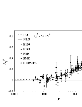
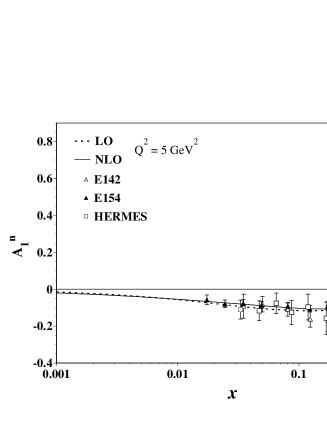
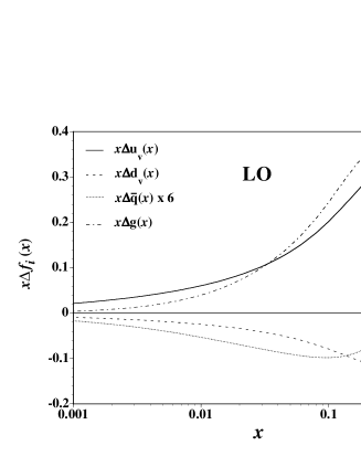
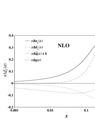
From the $\chi^{2}$ analysis, we obtain the results with $\chi^{2}$ = 322.6 in the LO case, and $\chi^{2}$ = 300.4 in the NLO case for 375 data points. The NLO $\chi^{2}$ is significantly smaller than the LO one. It suggests that the NLO analysis is necessary for precise analysis. The obtained $A_{1}$ for the proton and for the neutron at $Q^{2}$ = 5.0 GeV² are shown in Fig.1 with the experimental data. Although the comparison is not straightforward because the data are taken at various $Q^{2}$, the obtained parameters reproduce the data well both in the LO and the NLO case. Figure 2 show the obtained polarized parton distribution functions at $Q^{2}$ = 1.0 GeV². In our analysis, the first moment of $\Delta u_{v}$ ($\Delta d_{v}$) is fixed by positive (negative) value and the obtained distribution becomes positive (negative). Furthermore, antiquark and gluon distributions become negative and positive, respectivly.

         

Figure 1: Spin asymmetries $A_{1}$ for the proton (left figure) and neutron (right figure).

         

Figure 2: Obtained polarized distributions at $Q^{2}$ = 1.0 GeV².

For these distributions, quark spin content becomes $\Delta\Sigma$ = 0.201 for LO and $\Delta\Sigma=0.051$ for NLO at $Q^{2}$=1.0 GeV². The NLO $\Delta\Sigma$ is significantly smaller than the LO one. It is also smaller than the generally quoted values in other analyses that range in 0.1 $\sim$ 0.3. The difference of $\Delta\Sigma$ comes mainly from the difference of $\Delta\bar{q}$ in the small-$x$ region. Because we don’t have a small-$x$ data at this stage, we should fix the small-$x$ behavior of $\Delta\bar{q}$ from theoretical suggestions. We perform $\chi^{2}$ fitting by fixing the parameter $\alpha_{\bar{q}}$, which controls the small-$x$ behavior of $\Delta\bar{q}$, to $\alpha_{\bar{q}}$ = 1.0 and 1.6 according to the predictions of the Regge theory and the perturbative QCD. These values are rather larger than the value $\alpha_{\bar{q}}$ = 0.32 $\pm$ 0.22 which is obtained by the previous NLO analysis. As a result, we get $\Delta\Sigma$ = 0.241 ($\chi^{2}$ = 305.8) for $\alpha_{\bar{q}}$ = 1.0 and $\Delta\Sigma$ = 0.276 ($\chi^{2}$ = 323.5) for $\alpha_{\bar{q}}$ = 1.6. The obtained $\Delta\Sigma$ are larger than the previous NLO result and are within the usually quoted range. From these results, we find that $\Delta\Sigma$ is very sensitive to the small-$x$ behavior of the antiquark distributions. In order to determine the quark spin content precisely, the data in the small-$x$ region are needed. Because $\chi^{2}$ for the $\alpha_{\bar{q}}$ = 1.0 case is close to the one for the previous NLO, this set can be also considered as a good parametrization. Therefore, we propose three sets of distributions, LO, NLO with free $\alpha_{\bar{q}}$ (NLO-1), and NLO with $\alpha_{\bar{q}}$ = 1.0 (NLO-2), as AAC polarized distribution functions.

Finally, we briefly comment on the error estimate of the obtained distributions MM:ERROR . The uncertainties of our distributions can be estimated by using the error matrix which is obtained by MINUIT. The 1-$\sigma$ boundary of the distribution $F$ is given by

$$(\delta F)^{2}=\sum_{i}\sum_{j}\frac{\partial F}{\partial a_{i}}V_{ij}\frac{\partial F}{\partial a_{j}},$$ (3)

where, $V_{ij}$ is the error matrix element for parameters $a_{i}$ and $a_{j}$. This analysis is in progress and will be reported elsewhere.

Library

For practical application of our distributions, we provide a library program which is given as FORTRAN subroutine AACPDF(ISET, Q2, X, POLPDF, STRUCT). The users should call this subroutine in their programs with the input parameters ISET, Q2, and X. This library contains three sets of distributions, LO, NLO-1, and NLO-2, and the parameter ISET designates which set is used. When ISET=1, 2, or 3, the returned values are those in the LO, NLO-1, or NLO-2, respectively. The parameters Q2 and X specify $Q^{2}$ and Bjorken-$x$ at which the distributions are calculated. The allowed ranges are 1.0 GeV² $\leq Q^{2}\leq$ 10⁶ GeV² and 10^-9 $\leq x\leq$ 1.0. The obtained values are returned by the arrays POLPDF($-$3:3) and STRUCT(3). The available polarized parton distribution functions and the structure functions are listed in Table 1. It should be noted that the returned values are the distributions and the structure functions multiplied by $x$.

Table 1: Available distributions and structure functions.

I	POLPDF(I)	STRUCT(I)
-3	$\bar{s}$ quark [$x\Delta\bar{s}(x,Q^{2})$ = $x\Delta s(x,Q^{2})$)]	—
-2	$\bar{d}$ quark [$x\Delta\bar{d}(x,Q^{2})$ = $x\Delta d_{sea}(x,Q^{2})$]	—
-1	$\bar{u}$ quark [$x\Delta\bar{u}(x,Q^{2})$ = $x\Delta u_{sea}(x,Q^{2})$]	—
0	gluon [$x\Delta g(x,Q^{2})$]	—
1	u-valence quark [$x\Delta u_{v}(x,Q^{2})$]	$xg_{1}(x,Q^{2})$ for proton
2	d-valence quark [$x\Delta d_{v}(x,Q^{2})$]	$xg_{1}(x,Q^{2})$ for neutron
3	s quark [$x\Delta s(x,Q^{2})$ = $x\Delta\bar{s}(x,Q^{2})$]	$xg_{1}(x,Q^{2})$ for deuteron

The distribution values are obtained by interpolating the grid data which are provided as DATA statements in the subroutine. The number of the grid points is 23 for the variable $Q^{2}$ and 68 for the variable $x$. Because the $Q^{2}$ dependence of the distributions is almost linear function of $t\equiv\ln Q^{2}$, we simply use the linear interpolation of $t$ for the variable $Q^{2}$. If $t^{\prime}$ is in the range $t_{i}\leq t^{\prime}<t_{i+1}$, the distributions at $t=t^{\prime}$ are approximated by

$$f(t^{\prime})\approx\frac{t_{i+1}-t^{\prime}}{t_{i+1}-t_{i}}f(t_{i})+\frac{t^{\prime}-t_{i}}{t_{i+1}-t_{i}}f(t_{i+1}).$$ (4)

On the other hand, the $x$ dependence of the distributions is rather complicated. Therefore, we use the cubic spline interpolation for the variable $x$. If $x^{\prime}$ is in the range $x_{i}\leq x^{\prime}<x_{i+1}$, the distributions at $x=x^{\prime}$ are approximated by

$$f(x^{\prime})\approx f(x_{i})+B_{i}(x^{\prime}-x_{i})+C_{i}(x^{\prime}-x_{i})^{2}+D_{i}(x^{\prime}-x_{i})^{3}.$$ (5)

Here, $B_{i}$, $C_{i}$, $D_{i}$ are the spline coefficients which can be calculated by the grid data. By using these interpolation methods and the grid data, the AACPDF returns the values of the polarized parton distribution functions and the structure functions $g_{1}$ at the specified $Q^{2}$ and $x$ point. We verified that the distributions obtained by the library reproduce well the results in Ref.MM:AAC00 .

AAC library can be downloaded from our web page MM:AACWEB . The subroutine AACPDF is in the file “ aac.f ”. This file also includes the subroutine SPLINE and the function ISERCH which are used in the AACPDF.

Summary

The polarized parton distribution functions have been determined by $\chi^{2}$ fitting to $A_{1}$ experimental data. As a result, we found that the NLO $\chi^{2}$ is significantly smaller than the LO one. It implies that the NLO analysis is important. In the NLO analysis, the obtained $\Delta\Sigma$ is rather smaller than the usually quoted values, and the differences come from the small-$x$ behavior of $\Delta\bar{q}$. In order to fix $\Delta\Sigma$ precisely, the small-$x$ measurements are required. We propose three sets of AAC distributions, LO, NLO-1 ($\alpha_{\bar{q}}$ : free), and NLO-2 ($\alpha_{\bar{q}}$ = 1.0 fixed). The FORTRAN library is provided for calculating the AAC distributions numerically. This library is useful for practical application of the AAC distributions and available at our web site MM:AACWEB .