Abstract

We analize the renormalization group equations of supersymmetric QCD with $N=1$ for the evolution of parton distributions. For this purpose we develope a simple recursive algorithm in x-space to include both regular regions and supersymmetric regions in the evolution in the step approximation. Supersymmetric distributions are generated within a radiative model, with vanishing initial conditions for the superpartners. Here we focus on a scenario with broken susy, characterized by a lighter gluino coupled to the standard evolution and a decoupled scalar quark. Predictions for the all the distributions are presented.

1 Introduction

The study of the QCD scaling violations is an important chapter of high energy physics and a very important tool for the analysis of future data at the LHC. At large energy and momentum transfers, the underlying quark-gluon dynamics is light-cone dominated and controlled by a mechanism of collinear radiative emission described by logarithmic corrections to the lowest order cross section. In this picture, based on the parton model, initial quark states are assumed to be massless and the running of the coupling is linked to the number of flavours $n_{f}$ included in the evolution. Crossing intermediate thresholds opens up new channels and new dynamics. There is a widely used formalism of perturbative QCD that we think is worth to extend to the supersymmetric case and which might be useful for experimental searches of supersymmetry at the LHC. The picture is particularly appealing if a “supersymmetric content “ of the proton is found. However, predictions tied to this picture may be used to rule out a possible light gluino and/or a light squark. Other applications involve the study of nucleon collisions with the atmosphere as in Ultra High Energy Cosmic Rays, where the center of mass energy of the primaries can reach several hundreds of TeV’s.

This formalism involves the study of scaling violations induced on the initial state by the opening of supersymmetric channels prior to reaching the hard scattering phase. The analysis requires the notion of supersymmetric parton distributions, supersymmetric factorization formulas for supersymmetric DIS and (susy) hadron-hadron collisions on which we elaborate in detail. We remark that supersymmetric versions of parton distributions are easy to define, by a natural generalization of the usual DIS approach. The phenomenological validity of these extensions are clearly linked to the possibility of detecting scaling violations in precision measurements of final states in p-$\bar{p}$ collisions, for instance in Drell Yan, or in other processes with a distinct final state. With this analysis in perspective we start developing accurate tools that we will use in a separate work for a quantification of rates for gluino/squarks effects at the LHC. Although there is no evidence of supersymmetry at current energies, or of supersymmetry coming from the initial state, quantifying with accuracy these effects we believe, is still an interesting task. These studies are also of direct theoretical relevance, since they tell us more specifically how to merge the usual parton model dynamics with the new elementary states that supersymmetry predicts.

In this paper we start analizing these issues and make a first step toward quantifying the impact of supersymmetry in the initial state. Our analysis, in this paper, is focused on the supersymmetric DGLAP evolution, which is more involved compared to ordinary QCD. We solve the equations using a recursive algorithm that we formulate and that we have tested which allows to perform a direct match between the various regions of the evolution as we increase the factorization scale and allow for new (supersymmetric) channels. Part of the analysis is of technical nature and several sections deal with the implementation of the method. We then study in 2 final sections the implications of the susy evolution and compare it to the standard QCD one. Other aspects of the evolution, including some applications for collider processes will be analized in a companion paper.

2 The Method

Before moving to Supersymmetric QCD (SQCD), we briefly illustrate the method as it applies to the case of ordinary QCD. This simpler case will help us establish notations that will be later extended to the supersymmetric evolution. We build on previous work of Rossi [3], which has been used before in the previous literature [9, 8], although never fully documented in its code implementation. We combine that method, originally suggested for QCD, with recent approaches that use an analytic evaluation of the convolution integrals (“weights”) [6], and generalize it to SQCD. A recently application to QCD in next-to-leading order (NLO) of this approach has been implemented by Chuvakin and Smith [7] in their analysis of an evolution scheme with a varying number of flavours. To make the discussion self-contained, we have elaborated in some detail on the method in an appendix.

The two-loop running of the coupling constant is defined by

$${\alpha(Q_{0}^{2})\over 2\pi}={2\over\beta_{0}}{1\over\ln(Q^{2}/\Lambda^{2})}\left(1-{\beta_{1}\over\beta_{0}}{\ln\ln(Q^{2}/\Lambda^{2})\over\ln(Q^{2}/\Lambda^{2})}+O({1\over\ln^{2}(Q^{2}/\Lambda^{2})})\right)$$ (1)

where

$$\beta_{0}={11\over 3}C_{G}-{4\over 3}T_{R}n_{f}$$

$$\beta_{1}={34\over 3}C_{G}^{2}-{10\over 3}C_{G}n_{f}-2C_{F}n_{f},$$ (2)

where

$$C_{G}=N,\,\,\,\,\,\,\,C_{F}={N^{2}-1\over 2N},\,\,\,\,\,\,\,\,T_{R}={1\over 2}$$ (3)

and N is the number of colours while $n_{f}$ is the number of flavours.

The solution for the running coupling is given by

$$\alpha(t) = {\alpha(0)\over 2\pi}e^{-\beta_{0}/2t}$$ (4)

with $\alpha(Q_{0}^{2})\equiv\alpha(0)$, and $Q_{0}$ denoting the initial scale at which the evolution starts. The evolution equations are of the form

$$Q^{2}{d\over dQ^{2}}{q_{i}}^{(-)}(x,Q^{2}) = {\alpha(Q^{2})\over 2\pi}P_{(-)}(x,\alpha(Q^{2}))\otimes q_{i}^{(-)}(x,Q^{2})$$

$$Q^{2}{d\over dQ^{2}}\chi_{i}(x,Q^{2}) = {\alpha(Q^{2})\over 2\pi}P_{(-)}(x,\alpha(Q^{2}))\otimes\chi_{i}(x,Q^{2}),$$

with

$$\chi_{i}(x,Q^{2})={q_{i}}^{(+)}(x,Q^{2})-{1\over n_{F}}q^{(+)}(x,Q^{2})$$ (6)

for the non-singlet distributions and

$$Q^{2}{d\over dQ^{2}}\left(\begin{array}[]{c}q^{(+)}(x,Q^{2})\\ G(x,Q^{2})\end{array}\right)=\left(\begin{array}[]{cc}P_{qq}(x,Q^{2})&P_{qg}(x,Q^{2})\\ P_{gq}(x,Q^{2})&P_{gg}(x,Q^{2})\end{array}\right)\otimes\left(\begin{array}[]{c}q^{(+)}(x,Q^{2})\\ G(x,Q^{2})\end{array}\right)$$ (13)

for the singlet sector.

We have defined, as usual

$$q_{i}^{(-)}=q_{i}-\bar{q}_{i},\,\,\,\,\,q^{(+)}_{i}=q_{i}+\bar{q}_{i},\,\,\,\,\,\,q^{(+)}\equiv\Sigma=\sum_{i=1}^{n_{f}}q^{(+)}_{i}.$$ (15)

We introduce the evolution variable

$$t=-{2\over\beta_{0}}\ln{\alpha(Q^{2})\over\alpha(Q_{0}^{2})}$$ (16)

which replaces $Q^{2}$. The evolution equations are then rewritten in the form

$${d\over dt}q_{i}^{(-)}(t,x) = \left(P^{(0)}(x)+{\alpha(t)\over 2\pi}R_{(-)}(x)+...\right)\otimes q_{i}^{(-)}(t,x)$$ (17)

$$Q^{2}{d\over dt}\chi_{i}(x,Q^{2}) = \left(P^{(0)}(x)+{\alpha(t)\over 2\pi}R_{(+)}(x)\right)\otimes\chi_{i}(x,Q^{2}),$$ (18)

$${d\over dt}\left(\begin{array}[]{c}q^{(+)}(t,x)\\ G(x,t)\end{array}\right) = \left(P^{(0)}(x)+{\alpha(t)\over 2\pi}R(x)+...\right)\otimes\left(\begin{array}[]{c}q^{(+)}(x,t)\\ G(x,t)\end{array}\right).$$ (23)

In the new variable $t$, the kernels of the evolution take the form

$$R_{(\pm)}(x) = P^{(1)}_{(\pm)}(x)-{\beta_{1}\over 2\beta_{0}}P^{(0)}_{V}(x)$$

$$R(x) = P^{(1)}(x)-{\beta_{1}\over 2\beta_{0}}P^{(0)}(x).$$ (24)

Equations (17) and (18) are solved independently for the variables $q_{i}^{(-)}$ and $\chi_{i}$ respectively. Finally, the solution $q^{(+)}$ of eq. (23) (or the singlet equation) is substitued into $\chi_{i}$ in order to obtain $q_{i}^{(+)}$.

The equations can be written down in terms of two singlet evolution operators $E_{\pm}(t,x)$ and initial conditions $\tilde{q}_{\pm}(x,t=0)\equiv\tilde{q}_{\pm}(x)$ as

$${d\over dt}E_{\pm}=P_{\pm}\otimes E_{\pm},$$ (25)

whose solutions are given by

$$q_{i}^{(-)}(t,x)=E_{(-)}\otimes\tilde{q}_{i}^{(-)}$$

$$\chi_{i}(t,x)=E_{(+)}\otimes\tilde{\chi}_{i}(x).$$ (26)

The singlet evolution for the matrix operator $E(x,t)$

$$\left(\begin{array}[]{cc}E_{FF}(x,t)&E_{FG}(x,t)\\ E_{GF}(x,t)&E_{GG}(x,t)\end{array}\right)$$ (29)

$${dE(x,t)\over dt}=P\otimes E(x,t)$$ (30)

is solved similarly as

$$\left(\begin{array}[]{c}q^{(+)}(t,x)\\ G(t,x)\end{array}\right)=E(t,x)\otimes\left(\begin{array}[]{c}\tilde{q}^{(+)}(x)\\ \tilde{G}(x)\end{array}\right).$$ (35)

The unpolarized leading order kernels are expanded in $\alpha$ as

$$P_{ij}(x,\alpha_{s})=\left({\alpha_{s}\over 2\pi}\right)P^{(0)}_{ij}(x)+\left({\alpha_{s}\over 2\pi}\right)^{2}P^{(1)}_{ij}(x)+...$$ (36)

Their LO expressions are given by

$$P^{(0)}_{qq,NS}=C_{F}\left(\frac{1+x^{2}}{1-x}\right)_{+}$$ (37)

for the non-singlet sector, and by

$$P^{(0)}_{qq}(x)=P^{(0)}_{qq,NS}$$

$$P^{(0)}_{qg}(x)=2T_{R}n_{f}\left(x^{2}+(1-x)^{2}\right)$$

$$P^{(0)}_{gq}(x)=C_{F}{1+(1-x)^{2}\over x}$$

$$P^{(0)}_{gg}(x)=2N_{c}\left({1\over(1-x)_{+}}+{1\over x}-2+x(1-x)\right)+{\beta_{o}\over 2}\delta(1-x)$$ (38)

in the singlet sector. Some simple identities for the “plus’ $(+)$ distributions and their definition are given in the appendix.

In the actual numerical solution of the equation, one would like to have at hand a recursion relation which can be implemented in a computer program dynamically at run-time. In order to develope recursion relations we proceed as follow. We first observe that as far as we are not resumming double logarithms in $Q$ and $x$, the solution eq. (18) can be expanded as a series of convolution products

$$q(x,t)=q_{0}(x)+tP\otimes q_{0}(x)+\frac{t^{2}}{2!}P\otimes P\otimes q_{0}(x)+...$$ (39)

and transformed into a recursion relation for some coefficients $C_{N}(x)$

$$C_{0}(x) = \delta(x-1)$$

$$C_{N+1} = P\otimes C_{N}(x)$$ (40)

equivalent to the expansion for the evolution operator

$$E(x,t)=\sum_{n=0}^{\infty}C_{N}(x)\frac{t^{n}}{n!}.$$ (41)

Written as a recursion relation, the equation is as easy to implement as a calculation in moment space, but with no need to perform any moment inversion. The possibility of using this expansion as an alternative way to evolve parton distributions fast and with accuracy especially for larger sets of coupled equations, such as for supersymmetric theories, is the subject of the following sections. Specifically, Rossi’s ansatz [3], originally introduced in the context of the photon structure funtion, differs from (41) only by an over all normalization $C_{N}=(-1)^{N}\left(2/\beta_{0}\right)^{N}$

$${A}_{0}^{NS}(x)=\sum_{n=0}^{\infty}{{A}^{NS}_{n}(x)\over n!}\log^{n}\left({\alpha(m_{2\lambda})\over\alpha(Q_{0})}\right).\\$$

Connecting this expansion to other expansions is also pretty straightforward. A very elegant basis in which to expand is the Laguerre basis, introduced by Furmanski and Petronzio [5]. A relation between Rossi’s basis and the FP basis can also be derived but the result is not particularly illuminating.

Inserting the expansion (2) into the evolution equation one gets some recursion relations for the functions $A_{n+1}(x)$ in terms of the $A_{n}(x)$. These are obtained by comparing left hand side and right hand side of the evolution equations after equating the logarithmic powers with a running strong coupling constant $\alpha(Q^{2})$. A pretty detailed study in the polarized case can be found in ref. [9]. For computational purposes, the recursion relations for the evaluation of the $A_{n}(x)$’s can be implemented in various ways. The one that we have implemented involves the direct solution of the recursion relations as illustrated below. In leading order in $\alpha(Q^{2})$ in QCD we get for the unpolarized kernels

$$\tilde{A}_{n+1}^{V,\pm}(x) = \tilde{A}_{n}^{V,\pm}(x)\left[-\frac{3C_{F}}{\beta^{S}_{0}}-\frac{4C_{F}}{\beta^{S}_{0}}\ln(1-x)\right]$$ (42)

$$+ \frac{2C_{F}}{\beta^{S}_{0}}\int^{1}_{x}\frac{dy}{y}(1+z)A_{n}^{V}(y)-\frac{4C_{F}}{\beta^{S}_{0}}\int^{1}_{x}\frac{dy}{y}\frac{yA_{n}^{V}(y)-xA_{n}^{V}(x)}{y-x}$$

int the non-singlet case and

$$A_{n+1}^{q+}(x) = A_{n}^{q+}(x)\left[-\frac{3C_{F}}{\beta_{0}}-\frac{4C_{F}}{\beta_{0}}\ln(1-x)\right]$$ (43)

$$+ \frac{2\,C_{F}}{\beta_{0}}\int^{1}_{x}\frac{dy}{y}(1+{x\over y})A_{n}^{q+}(y)-{2\over\beta_{0}}n_{f}\int_{x}^{1}\frac{dy}{y}\left\{2\frac{x}{y}{(x-y)\over y}+1\right\}A_{n}^{G}(y)$$

$$- \frac{4C_{F}}{\beta_{0}}\int^{1}_{x}\frac{dy}{y}\frac{yA_{n}^{q+}(y)-xA_{n}^{q+}(x)}{y-x}$$

$$A_{n+1}^{G}(x) = \frac{-2}{\beta_{0}}C_{F}\int_{x}^{1}\frac{dy}{y}\frac{1+(1-z)^{2}}{z}A_{n}^{q+}(y)$$

$$- \frac{4N_{c}}{\beta_{0}}\int_{x}^{1}\frac{dy}{y}\frac{yA_{n}^{G}(y)-xA_{n}^{G}(x)}{y-x}-\frac{4N_{c}}{\beta_{0}}\ln(1-x)A_{n}^{G}(x)$$

$$- \frac{4N_{c}}{\beta_{0}}\int_{x}^{1}\frac{dy}{y}\left\{\frac{1}{z}-2+z(1-z)\right\}A_{n}^{G}(y)-A_{n}^{G}(x)$$

in the singlet. Extensions to the NLO case of this approach are pretty straightforward, and the procedure will be more clear once we will discuss its implementation to solve the Supersymmetric DGLAP (SDGLAP) equations.

3 Supersymmetric scaling violations

In $N=1$ QCD gluons have partners called gluinos (here denoted by $\lambda$) and left- and right-handed quarks have complex scalar partners (squarks) which we denote as $\tilde{q_{L}}$ and $\tilde{q_{R}}$ with $\tilde{q}=\tilde{q}_{L}+\tilde{q}_{R}$ (for left-handed and right-handed squarks respectively).

The interaction between the elementary fields are described by the $SU(3)$ color gauge invariant and supersymmetric lagrangean

$${\cal L}=-{1\over 4}G_{\mu\nu}^{a}G^{\mu\nu}_{a}+{1\over 2}\bar{\lambda}_{a}\left(i\not{D}\right)\lambda)_{a}$$

$$+\bar{q}_{i}I\not{D}q_{i}+D_{\mu}\tilde{q}_{R}D^{\mu}\tilde{q}^{R}+D_{\mu}\tilde{q}_{L}D^{\mu}\tilde{q}^{L}+ig\sqrt{2}\left(\bar{\lambda^{a}}_{R}\tilde{q_{iL}^{\dagger}}T^{a}q_{Li}+\bar{\lambda^{a}}_{L}\tilde{q_{iR}^{\dagger}}T^{a}q_{Ri}-{\tt h.\,\,\,c.}\right)$$

$$-{1\over 2}g^{2}\left(\tilde{q_{Li}^{\dagger}}T^{a}\tilde{q_{Li}}-\tilde{q_{Ri}^{\dagger}}T^{a}\tilde{q_{Ri}^{\dagger}}\right)^{2}+{\tt mass\,\,\,\,terms},$$

where $a$ runs over the adjoint of the color group and $i$ denotes the number of flavours over which we sum.

Past studies of these effects lead to the conclusion that the information that supersymmetric initial states carry along the evolution can be easily absorbed into scaling violations coming from ordinary QCD. These studies require the knowledge of the matrix of the anomalous dimensions (for all the moments), or of the corresponding Altarelli-Parisi (DGLAP) kernels. We recall that the leading and next-to-leading anomalous dimensions are known [2] since long ago, at least in the case of partial supersymmetry breaking, in a scenario characterized by a light gluino and a decoupled scalar quark (we present in an appendix the leading order form of these kernels for completeness). In this work we consider the possibility of a radiatively generated gluino distributions, in analogy with the case of standard QCD for the gluons. In fact, in QCD one can use a simple model of the distributions at low $Q$ $(Q=Q_{0})$ and run the DGLAP equations up in energy in order to generate distributions of gluons at any higher scale $Q_{f}$. Of course, it is well known that in QCD such initial evolution scale is model dependent. Various amplitudes at higher energy emerge, depending on the underlying assumptions on the form of their initial shapes.

This approach has been widely used in the literature and can be a way to connect low energy quark models -which have no gluons but a phenomenological confining potential - to true QCD scattering amplitudes. One can assume a zero distribution of glue at the lowest scale, or a model dependent non zero one, and then use the evolution equations to dress the matrix elements describing the distributions by logarithmic corrections. Once the final scale -here identified as the factorization scale of the process - is reached, the distributions are convoluted with the usual -on shell- parton cross sections to generate the full hadronic cross section.

In hadronic collisions, $Q_{f}$ is usually a fraction of the center-of-mass energy, or a fraction of the large $p_{T}$ of the final state jets. It is not uniquely identified and a different choice of $Q_{f}$ underscores a drastic sensitivity of the expansion on this scale.

Alternative choices for density of the constituents at low $Q$ are also possible, but, ultimately, whatever the choice for the parton structure, it has to match the scattering data available from DIS and colliders experiments. In the case of exact SQCD, it is natural to parametrize the parton distributions, now with a susy content in the form

$$F_{2}(x,Q^{2}) = xe_{i}^{2}\left(q_{i}(x,Q^{2})+\bar{q}_{i}(x,Q^{2})+\tilde{q}_{iR}(x,Q^{2})+\bar{\tilde{q}}_{iR}(x,Q^{2})\right.$$ (45)

$$\left.\tilde{q}_{iL}(x,Q^{2})+\bar{\tilde{q}}_{iL}(x,Q^{2})\right),$$

where the new elementary constituents (squarks and gluons) can be vanishing at low $Q$ and be radiatively generated by the evolution, similarly to the gluon case (in standard QCD) contemplated above. In the case of a broken susy, the form of $F_{2}$ does not change from the standard QCD form.

A gluino or a squark parton distribution (a more detailed analysis will be presented elsewhere) is the exact correspondent of a gluon or a quark parton distribution, namely a light-cone dominated diagonal (non local) correlation function in spacetime, Fourier transformed to (Bjorken) x-space.

Similarly to the QCD case, in the case of exact $N=1$ supersymmetry we define singlet and non-singlet distributions

$$q_{v}(x,Q^{2}) = \sum_{i=1}^{n_{f}}\left({q}_{i}(x,Q^{2})-{\bar{q}}_{i}(x,Q^{2})\right),$$

$$\tilde{q}_{V}(x,Q^{2}) = \sum_{i=1}^{n_{f}}\left(\tilde{q}_{i}(x,Q^{2})-\tilde{\bar{q}}_{i}(x,Q^{2})\right)$$

$$q^{+}(x,Q^{2}) = \sum_{i=1}^{n_{f}}\left({q}_{i}(x,Q^{2})+\bar{q}_{i}(x,Q^{2})\right)$$

$$\tilde{q}^{+}(x,Q^{2}) = \sum_{i=1}^{n_{f}}\left(\tilde{q}_{i}(x,Q^{2})+\tilde{\bar{q}}_{i}(x,Q^{2})\right).$$ (46)

The evolution equations can be separated in two non-singlet sectors and a singlet one. The non-singlet are

$$Q^{2}{d\over dQ^{2}}q_{V}(x,Q^{2}) = {\alpha(Q^{2})\over 2\pi}\left(P_{qq}\otimes q_{V}+P_{q\tilde{q}}\otimes\tilde{q_{V}}\right)$$

$$Q^{2}{d\over dQ^{2}}\tilde{q}_{V}(x,Q^{2}) = {\alpha(Q^{2})\over 2\pi}\left(P_{\tilde{q}q}\otimes q_{V}+P_{\tilde{q}\tilde{q}}\otimes\tilde{q_{V}}\right),$$

and the singlet, which mix $q_{V}$ and $\tilde{q}_{V}$ with the gluons and the gluinos are

$$Q^{2}{d\over dQ^{2}}\left[\begin{array}[]{c}G(x,Q^{2})\\ \lambda(x,Q^{2})\\ q^{+}(x,Q^{2})\\ \tilde{q}^{+}(x,Q^{2})\end{array}\right]=\left[\begin{array}[]{llll}P_{GG}&P_{G\lambda}&P_{Gq}&P_{G\tilde{q}}\\ P_{\lambda G}&P_{\lambda\lambda}&P_{\lambda q}&P_{\lambda\tilde{q}}\\ P_{qG}&P_{q\lambda}&P_{qq}&P_{qs}\\ P_{sG}&P_{s\lambda}&P_{\tilde{q}q}&P_{\tilde{q}\tilde{q}}\end{array}\right]\otimes\left[\begin{array}[]{c}G(x,Q^{2})\\ \lambda(x,Q^{2})\\ q^{+}(x,Q^{2})\\ \tilde{q}^{+}(x,Q^{2})\end{array}\right].$$ (48)

There are simple ways to calculate the kernel of the SDGLAP evolution by a simple extension of the usual methods. The changes are primarily due to color factors. There are also some basic supersymmetric relations which have to be satisfied that will be analized below. They are generally broken in the case of decoupling. We recall that the supersymmetric version of the $\beta$ function is given at two-loop level by

$$\beta_{0}^{S} = \frac{1}{3}\left(11C_{A}-2n_{f}-2n_{\lambda}\right)$$

$$\beta_{1}^{S} = \frac{1}{3}\left(34C_{A}^{2}-10C_{A}n_{f}-10C_{A}n_{\lambda}-6C_{F}n_{F}-6C_{\lambda}n_{\lambda}\right)$$ (49)

with $C_{\lambda}=C_{A}=N_{c}$ for the case of Majorana gluinos and the ordinary running of the coupling is replaced by its supersymmetric running

$${\alpha^{S}(Q_{0}^{2})\over 2\pi}={2\over\beta_{0}^{S}}{1\over\ln(Q^{2}/\Lambda^{2})}\left(1-{\beta_{1}^{S}\over\beta_{0}^{S}}{\ln\ln(Q^{2}/\Lambda^{2})\over\ln(Q^{2}/\Lambda^{2})}+O({1\over\ln^{2}(Q^{2}/\Lambda^{2})})\right).$$ (50)

The kernels are modified both in their coupling $(\alpha\to\alpha^{S})$ and in their internal structure (Casimirs, color factors, etc.) when moving from the QCD case to the SQCD case. In our conventions an index “S” stands for a supersymmetric component (regular, i.e. non supersymmetric, kernels do not carry such an index), but we will omit it when obvious.

4 Evolution and Matching

Susy is necessarily broken in the real world and therefore, the way the breaking occurs dictates both the mass spectrum and guides the structure of the QCD scaling violations as well. There are several parameters that appear in the evolution, $m_{\lambda}$ and $m_{\tilde{q}}$, the masses of the gluino and squarks, hence a complete analysis includes various scenarios, on which we briefly elaborate. In a realistic scenario with a broken susy, the squarks have much larger mass compared to the quarks and the gluinos have a Dirac or Majorana mass $m_{\lambda}$ (or a combination them). In our case, in order to establish the evolution scales which are of phenomenological interest, it is convenient to assume 1) that the scalar quark decouples from the evolution and 2) that the 2-gluino production threshold $m_{2\lambda}=2m_{\lambda}$ is the intermediate scale, separating in $Q^{2}$ the regular QCD region from the supersymmetric one. In this scenario some of the splitting functions - specifically $P_{q\lambda}$ and $P_{\lambda q}$ - are zero, since no collinear emission is associated with massive partons, unless the symmetry is effectively restored.

We impose the separation condition

$$Q_{0}<m_{2\lambda}<Q$$ (51)

and only one non singlet evolution equation is considered

$$Q^{2}{d\over dQ^{2}}q_{V}(x,Q^{2}) = {\alpha(Q^{2})\over 2\pi}P_{qq}\otimes q_{V}.$$

The simplified singlet equations, which mix $q_{V}$ and $\tilde{q}_{V}$ with the gluons and the gluinos become

$$Q^{2}{d\over dQ^{2}}\left[\begin{array}[]{c}G(x,Q^{2})\\ \lambda(x,Q^{2})\\ q(x,Q^{2})\end{array}\right]=\left[\begin{array}[]{lll}P_{GG}&P_{G\lambda}&P_{Gq}\\ P_{\lambda G}&P_{\lambda\lambda}&P_{\lambda q}\\ P_{qG}&P_{q\lambda}&P_{qq}\\ \end{array}\right]\otimes\left[\begin{array}[]{c}G(x,Q^{2})\\ \lambda(x,Q^{2})\\ q(x,Q^{2})\end{array}\right].$$ (53)

Formally, we can write down the expression of the complete solution in the form

$$q_{NS}(x,Q_{f}^{2}) = q(x,Q_{0}^{2})+\int_{{Q_{0}}^{2}}^{m_{2\lambda}^{2}}d\ln Q^{2}\,\,P_{NS}(x,\alpha(Q^{2})\otimes q_{NS}(x,Q^{2})$$

$$+ \int_{m_{2\lambda}^{2}}^{{Q_{f}}^{2}}d\ln Q^{2}\,\,\,\,\,P_{NS}(x,\alpha(Q^{2}))\otimes q_{NS}(x,Q^{2})$$

for the non-singlet equation and

$$\left[\begin{array}[]{c}G(x,Q_{f}^{2})\\ \lambda(x,Q_{f}^{2})\\ q(x,Q_{f}^{2})\end{array}\right] = \left[\begin{array}[]{c}G(x,Q_{0}^{2})\\ 0\\ q(x,Q_{0}^{2})\end{array}\right]+\int_{Q^{2}}^{m_{2\lambda}^{2}}d\ln Q^{2}P(x,\alpha(Q))\otimes\left[\begin{array}[]{c}G(x,Q^{2})\\ 0\\ q(x,Q^{2})\end{array}\right]$$ (64)

$$+ \int_{m_{2\lambda}^{2}}^{Q_{f}^{2}}d\ln Q^{2}P^{S}(x,\alpha^{S}(Q^{2}))\otimes\left[\begin{array}[]{c}G(x,Q^{2})\\ 0\\ q(x,Q^{2})\end{array}\right]$$ (68)

for the singlet one. In analogy with eq. (2), now we introduce supersymmetric coefficients $\tilde{A}^{n}(x)$ beside the usual non supersymmetric $A_{n}(x)$, and impose recursion relations on the initial ansatz $q(x,Q_{0}^{2})$ of the form

$$A^{NS}_{0}(x) = \delta(1-x)\otimes q(x,Q_{0}^{2})=q(x,Q_{0}^{2}),$$ (69)

$$A^{NS}_{n+1} = -{2\over\beta_{O}}P_{qq}\otimes A_{n},$$ (70)

$$\tilde{A}_{0}^{NS}(x) = \sum_{n=0}^{\infty}{{A}^{NS}_{n}(x)\over n!}\log^{n}\left({\alpha(m_{2\lambda})\over\alpha(Q_{0})}\right),$$ (71)

$$\tilde{A}^{NS}_{n+1} = -{2\over\beta_{O}^{S}}P_{qq}^{S}\otimes\tilde{A}^{NS}_{n}$$

$n=1,2,...$, which solve the equation in the non-singlet sector.

In the singlet sector we get the solution

$$\left[\begin{array}[]{c}G(x,Q_{0}^{2})\\ \lambda(x,Q_{0}^{2})\\ q^{+}(x,Q_{0}^{2})\end{array}\right] = \left[\begin{array}[]{c}G(x,Q_{0}^{2})\\ 0\\ q(x,Q_{0}^{2})\end{array}\right]+\sum_{n=1}^{\infty}\frac{1}{n!}\left[\begin{array}[]{c}A_{n}^{g}(x,Q^{2})\\ A_{n}^{\lambda}(x,Q^{2})\\ A_{n}^{q}(x,Q^{2})\end{array}\right]\,\,\log^{n}\left({\alpha(m_{2\lambda})\over\alpha(Q_{0})}\right)$$ (82)

$$+ \sum_{n=1}^{\infty}\frac{1}{n!}\left[\begin{array}[]{c}\tilde{A}_{n}^{g}(x,Q^{2})\\ \tilde{A}_{n}^{\lambda}(x,Q^{2})\\ \tilde{A}_{n}^{q}(x,Q^{2})\end{array}\right]\,\,\log^{n}\left({\alpha(Q)\over\alpha(m_{2\lambda})}\right),$$ (86)

constructed recursively through the relations

$$\left[\begin{array}[]{c}{A}_{0}^{g}(x)\\ {A}_{0}^{\lambda}(x)\\ {A}_{0}^{q}(x)\end{array}\right] = \left[\begin{array}[]{c}G(x,Q_{0}^{2})\\ 0\\ q(x,Q_{0}^{2})\end{array}\right],$$ (94)

$$\left[\begin{array}[]{c}{A}_{n+1}^{g}(x,Q^{2})\\ {A}_{n+1}^{\lambda}(x,Q^{2})\\ {A}_{n+1}^{q}(x)\end{array}\right] = -\left(\frac{2}{\beta_{0}}\right)P\otimes\left[\begin{array}[]{c}{A}_{n}^{g}(x)\\ {A}_{n}^{\lambda}(x)\\ {A}_{n}^{q}(x)\end{array}\right]$$ (101)

$$\left[\begin{array}[]{c}\tilde{A}_{0}^{g}(x)\\ \tilde{A}_{0}^{\lambda}(x)\\ \tilde{A}_{0}^{q}(x)\end{array}\right] = \sum_{n=0}^{\infty}\frac{1}{n!}\left[\begin{array}[]{c}\tilde{A}_{n}^{g}(x)\\ \tilde{A}_{n}^{\lambda}(x)\\ \tilde{A}_{n}^{q}(x)\end{array}\right]\,\,\log^{n}\left({\alpha(m_{2\lambda})\over\alpha(Q_{0})}\right)$$ (108)

$$\left[\begin{array}[]{c}\tilde{A}_{n+1}^{g}(x)\\ \tilde{A}_{n+1}^{\lambda}(x)\\ \tilde{A}_{n+1}^{q}(x)\end{array}\right] = -\left(\frac{2}{\beta_{0}^{S}}\right)P^{S}\otimes\left[\begin{array}[]{c}\tilde{A}_{n}^{g}(x)\\ \tilde{A}_{n}^{\lambda}(x)\\ \tilde{A}_{n}^{q}(x)\end{array}\right],$$ (115)

$n=1,2,...$, having used a vanishing gluon density at the starting point of the supersymmetric evolution.

5 Supersymmetric Relations

An exact supersymmetric scenario is probably interesting only for analizing theoretical issues concerning the evolution, or to study the shape of the distributions at extremely high energies, when, again, all the supersymmetric partners effectively become mass degenerate. This scenario can take place at few TeV’s or at several TeV’s, depending upon the assumptions underlying the way supersymmetry is restored. Here we simply focus our analysis on a light, up to an intermediate-mass Majorana gluino. Other aspects of the evolution, such as the interplay of Dirac and Majorana gluinos and the impact of various patterns of susy breaking will be considered elsewhere.

As we have already mentioned, the study of the anomalous dimensions - in leading order - for $N=1$ QCD can be found in [1] and now we are going to elaborate on that.

We recall that in a regularization scheme which is manifestly supersymmetric there are some supersymmetric relations which are satisfied by the anomalous dimensions. This is true, for instance, in the Dimensional Reduction $\overline{DR}$ scheme. We recall that to leading order the $\overline{MS}$ scheme and the supersymmetric $\overline{DR}$ scheme give coincident results. We recall that in the $\overline{DR}$ scheme the traces are kept in 4 dimensions, and the chiral projectors are treated as usual, with a completely anticommuting $\gamma_{5}$. The loop momenta are evaluated in n-dimensions. In other schemes, such as the t’Hooft-Veltman scheme, $\gamma_{5}$ is instead partially anticommuting. The $\overline{MS}$ scheme for chiral states is usually based on this second definition. The relation between the two schemes is to leading order

$$P^{(0)}_{\overline{MS}}=P^{(0)}_{\overline{DR}}$$ (117)

valid both for the non singlet and the singlet anomalous dimensions.

The same is true also for the factorization scheme dependence of the coefficient functions. As for the coupling constant, the definition of $\alpha$ in the two schemes, the expression of $\alpha_{\overline{MS}}$ can be used also in the $\overline{DR}$ scheme as far as the $\Lambda_{QCD}$ scales of the two schemes are related by $\Lambda_{\overline{DR}}=\Lambda_{\overline{MS}}exp\left(C_{A}/6\beta_{0}\right)$. This last change is tiny and will be neglected.

Part of the supersymmetric kernels can be obtained at this order by a simple change of group factors, from the standard QCD kernels. For instance, the substitutions $C_{F}\to C_{\lambda}$ ($C_{F}=(N_{c}^{2}-1)/(2N_{C})$) and $n_{f}\to n_{\lambda}$, allow us to obtain the kernels $(\lambda\lambda,\lambda g,g\lambda)$ from the ordinary kernels $(qq,qg,gq)$. We use $C_{\lambda}=C_{A}=N_{c}$, the number of colors. As for the choice of the type of representation for the gluino ( Majorana or Dirac), we recall that in the Dirac case we set $n_{\lambda}=2C_{A}$ while in the Majorana case $n_{\lambda}=C_{A}$. The organization of the terms in the splitting functions may differ from reference to reference, due to the various manipulations one can perform on the plus distributions.

The supersymmetry relations are given by

$$P_{gg}+P_{\lambda g}=P_{g\lambda}+P_{\lambda\lambda}\\$$ (118)

and by

$$P_{qg}+P_{\lambda q} = P_{gs}+P_{\lambda s}$$

$$P_{qg}+P_{sg} = P_{q\lambda}+P_{s\lambda}$$

$$P_{qq}+P_{sq} = P_{qs}+P_{ss}$$ (119)

In general, for a decoupled scalar quark, the only symmetry one would expect is eq. (118). In the case of Majorana gluinos, for a scenario with a decoupled squark, it is interesting to observe that this relation remains valid for $x<1$ as well. It can be extrapolated to include the $x=1$ point in the case of zero number of flavours (supersymmetric gluondynamics).

The evolution has to respect - both in the case of exact susy and of susy breaking - 1) baryon number conservation and 2) momentum conservation. There are two sum rules associated with these conserved quantities, which are generally used to constrain the phenomenological parametrizations of the distributions in direct applications. Below the $m_{2\lambda}$ threshold we need to satisfy the usual QCD relations

$$\int_{0}^{1}dx\left(xG(x,Q^{2})+xq^{(+)}(x,Q^{2})\right)=1$$ (120)

for momentum conservation and

$$\int_{0}^{1}dxq^{(-)}(x,Q^{2})=3$$ (121)

for baryon number conservation. These require that the anomalous dimensions satisfy the relations

$$\int_{0}^{1}xdx\left(P_{gi}(x)+P_{qi}(x)\right) = 0$$

$$\int_{0}^{1}dxP_{NS}(x) = 0,$$

respectively, where $i=q,g$. In leading order the second equation is simply

$$\int_{0}^{1}dxP^{(0)}_{qq}(x)=0.$$ (123)

Moving above the 2-gluino threshold the momentum sum rule becomes

$$\int_{0}^{1}dx\left(xG(x)+x\lambda(x)+xq^{(+)}(x)\right)=1$$ (124)

for momentum conservation, while eq. (121) remains unaltered. We get the new momentum sum rule (or second moment sum rule)

$$\int_{0}^{1}xdx\left(P_{gi}(x)+P_{qi}(x)+P_{\lambda i}\right) = 0,$$ (125)

with $i=q,g,\lambda$. The supersymmetric version of eq. (123) is simply obtained by replacing $P^{(0)}_{qq}(x)$ by it supersymmetric counterpart $P^{S\,(0)}_{qq}(x)$. It can be checked easily that the kernels in the appendix satisy these relations.

In the case of exact supersymmetry we need to keep into account the scalar quark contribution in both equations. In particular, the equation for the second moment becomes

$$\int_{0}^{1}x\,dx\left(xG(x)+x\lambda(x)+xq^{(+)}(x)+x\tilde{q}^{(+)}(x)\right)=1,$$ (126)

which implies that

$$\int_{0}^{1}xdx\left(P_{gi}(x)+P_{qi}(x)+P_{\lambda i}+P_{\tilde{q}i}\right) = 0,$$ (127)

with $i=q,g,\lambda,\tilde{q}$. As for baryon number conservation, equation (121) gets modified into

$$\int_{0}^{1}dx\left(q^{(-)}(x)+\tilde{q}^{(-)}(x)\right)=3$$ (128)

and using (LABEL:susyns) one gets two relations

$$\int_{0}^{1}dx\left(P^{S}_{qq}+P^{S}_{sq}\right) = 0$$

$$\int_{0}^{1}dx\left(P^{S}_{ss}+P^{S}_{qs}\right) = 0$$

(below we will drop the susy index $S$ in front of the kernels when obvious). The first relation in the equation above, for instance, clearly implies that the end point contributions in the ordinary $P_{qq}$ kernel are to be modified in order to insure conservation of baryon number. In the case of a susy breaking scenario such additional end-point contribution is trivially absent and the form of the $P_{qq}$ kernel remains the same, except for the replacement of $\alpha$ with $\alpha^{S}$, the supersymmetric coupling and $\beta_{0}$ with $\beta^{S}_{0}$.

6 Applications

In order to apply the formalism to SQCD we proceed by discussing the method for a scenario with a broken susy (decoupled squark). We proceed from the non singlet case, analizing in details the intermediate steps of the algorithm.

We start with a solution of the standard non-singlet DGLAP equation assuming the boundary condition $A_{0}^{V}(x)=q^{V}(x,Q_{0}^{2})$ and run the equation up to the gluino threshold and construct the coefficients recursively. We arrest the coefficient up to a desired order $(\bar{n})$, which can be as large as $30$. In general, the rate of convergence of the asymptotic expansion changes with the value of the momentum $Q$.

The solution is then constructed in the region $Q_{0}<Q<m_{2\lambda}$ as

$$q^{V}(x,m_{2\lambda})=\sum_{n=0}^{\bar{n}}{A^{V}_{n}(x)\over n!}\ln\left(\frac{\alpha(m_{2\lambda})}{\alpha(Q_{0})}\right)$$ (130)

and used as initial condition for the next stage of the evolution, which involves the region $m_{2\lambda}<Q<Q_{f}$, with $Q_{f}$ being the final evolution scale.

At the next stage, we set $\tilde{A}^{V}_{0}(x)=\delta(1-x)\otimes q^{V}(x,m_{2\lambda})$ and solve recursively using the supersymmetric version of the kernels. The strong coupling constant $\alpha(Q^{2})$ and its running are replaced by their supersymmetric version $\alpha^{S}(Q^{2})$, and so are the coefficients of the beta function $(\beta_{i}\to\beta_{i}^{s})$. Finally the solution is written down in the form

$$q^{V}(x,Q^{2}) = \sum_{n=0}^{\bar{n}}{A_{n}^{V}(x)\over n!}\log^{n}\left({\alpha(m_{2\lambda})\over\alpha(Q_{0})}\right)+\sum_{n=1}^{\bar{n}^{\prime}}{\tilde{A}_{n}^{NS}\over n!}\log^{n}\left({\alpha(m_{2\lambda})\over\alpha(Q)}\right)$$ (131)

where $\bar{n}^{\prime}$ is the index at which we arrest the supersymmetric recursion. In our implementation we have kept the values of $\bar{n}$ and $\bar{n}^{\prime}$ very close.

In the singlet case the procedure is not much different. We evolve according to the standard DGLAP equation in the region below the 2-gluino threshold, having set to zero the contribution from the gluino at the beginning (up to the supersymmetric threshold). This is equivalent to having set $A_{n}^{\lambda}(x)=0$ for any $n$, which means that in the region below $m_{2\lambda}$ there is no radiative production of gluinos in the initial stage. We iterate the recursion relations up to a given value $\bar{n}$ of the index $n$ with the standard DGLAP. The initial conditions for the next stage of the evolution are then fixed by the relations

$$\tilde{A}^{q+}_{0}(x) = q^{+}(x,m_{2\lambda}),$$ (132)

$$= \sum_{n=0}^{\bar{n}}{A^{q}_{n}(x)\over n!}\log^{n}\left(\frac{\alpha(m_{2\lambda})}{\alpha(Q_{0})}\right),$$

$$\tilde{A}^{g}_{0}(x) = G(x,m_{2\lambda})$$ (133)

$$= \sum_{n=0}^{\bar{n}}{A^{g}_{n}(x)\over n!}\log^{n}\left(\frac{\alpha(m_{2\lambda})}{\alpha(Q_{0})}\right)$$

$$\tilde{A}_{0}^{\lambda}(x) = \lambda(x,Q_{0}^{2})=0.$$

After this, we determine recursively the coefficients $\tilde{A}_{n}$ of the supersymmetric expansion

$$\tilde{A}_{n+1}^{q+} = -\frac{4C_{F}}{\beta_{0}^{S}}\int_{x}^{1}\frac{dy}{y}\frac{y\tilde{A}_{n}^{q+}(y)-x\tilde{A}_{n}^{q+}(x)}{y-x}$$

$$- \frac{4C_{F}}{\beta_{0}^{S}}\log(1-x)\tilde{A}_{n}^{q+}(x)+\frac{2C_{F}}{\beta_{0}^{S}}\int_{x}^{1}\frac{dy}{y}(1+z)\tilde{A}_{n}^{q+}(y)-\frac{3C_{F}}{\beta_{0}^{S}}\tilde{A}_{n}^{q+}(x)$$

$$- \frac{2n_{f}}{\beta_{0}^{S}}\int_{x}^{1}\frac{dy}{y}\left(1-2z+2z^{2}\right)\tilde{A}_{n}^{g}(y),$$

$$\tilde{A}_{n+1}^{\lambda}(x) = -4\frac{C_{\lambda}}{\beta_{0}^{S}}\int_{x}^{1}\frac{dy}{y}\frac{y\tilde{A}_{n}^{\lambda}(y)-x\tilde{A}_{n}^{\lambda}(x)}{y-x}$$ (136)

$$+ 2\frac{C_{\lambda}}{\beta_{0}^{S}}\int_{x}^{1}\frac{dy}{y}(1+z)\tilde{A}_{n}^{\lambda}(y)-\frac{3}{\beta_{0}^{S}}C_{\lambda}\tilde{A}_{n}^{\lambda}(x)$$

$$- \frac{2}{\beta_{0}^{S}}n_{\lambda}\int_{x}^{1}\frac{dy}{y}(1-2z+2z^{2}))\tilde{A}_{n}^{g}(y)-4\frac{C_{\lambda}}{\beta_{0}^{S}}\tilde{A}_{n}^{\lambda}(x)\log(1-x),$$

$$\tilde{A}_{n+1}^{g} = -\frac{2}{\beta_{0}^{S}}C_{F}\int_{x}^{1}\frac{dy}{y}\left(\frac{2}{z}-2+z\right)\tilde{A}_{n}^{q}(y)-\frac{2}{\beta_{0}^{S}}C_{\lambda}\int_{x}^{1}\frac{dy}{y}\left(\frac{2}{z}-2+z\right)\tilde{A}_{n}^{\lambda}(y)$$

$$-4\frac{C_{A}}{\beta_{0}^{S}}\int_{x}^{1}\frac{dy}{y}\frac{y\tilde{A}_{n}^{g}(y)-x\tilde{A}_{n}^{g}(x)}{y-x}-4\frac{C_{A}}{\beta_{0}^{S}}\log(1-x)\tilde{A}_{n}^{g}(x)$$

$$-4\frac{C_{A}}{\beta_{0}^{S}}\int_{x}^{1}\frac{dy}{y}\left(\frac{1}{z}-2+z(1-z)\right)\tilde{A}_{n}^{g}(y)-\tilde{A}_{n}^{g}(x).$$

Finally, we construct the solution in the form

$$f(x,Q^{2}) = \sum_{n=0}^{\bar{n}}{A^{f}_{n}(x)\over n!}\log^{n}\left({\alpha(m_{2\lambda})\over\alpha(Q_{0})}\right)+\sum_{n=1}^{\bar{n}^{\prime}}{\tilde{A}_{n}^{f}\over n!}\log^{n}\left({\alpha(Q_{f})\over\alpha(m_{2\lambda})}\right),$$

where we have arrested the supersymmetric recursion up to the index $\bar{n}^{\prime}$. Here $f(x,Q^{2})$ indicates a singlet quark, a gluon, or a gluino distribution, with $A_{n}^{f}(x)$ and $\tilde{A}^{f}_{n}(x)$ denoting their corresponding coefficients in the expansion. Singularities emerging from the lower integration point $(y=x)$ are the tricky part of the game, as expected, but can be handled with various techniques. They will be discussed briefly in the last section.

7 NLO Extensions

Let’s now move to a next-to-leading order (NLO) analysis of the evolution. Our discussion here is partial and does not include contributions due to the emergence of new anomalous dimensions as we move across the supersymmetric threshold. In recent work [7] it has been shown that in the ordinary distributions of quarks and gluons of QCD these effects are important, especially at small-x. These changes are expected to produce only a slight modification of the algorithm presented below, and simply amount to a modification of the boundary condition as we move across the $m_{2\lambda}$ point. They will not be analized any further in this work and will be assumed to be negligible. As a second point, we remark that the extension of the procedure outlined below is easy to generalize to the more general case of exact susy.

To NLO the ansatz becomes

$$q(x,Q^{2})=\sum_{n=0}^{\infty}\frac{A_{n}(x)}{n!}\log^{n}\left(\frac{\alpha(Q^{2})}{\alpha(Q_{0}^{2})}\right)+\alpha(Q^{2})\sum_{n=0}^{\infty}\frac{B_{n}(x)}{n!}\log^{n}\left(\frac{\alpha(Q^{2})}{\alpha(Q_{0}^{2}}\right)$$ (140)

and inserting the usual running of the coupling

$$\frac{d\alpha}{d\log(Q^{2})} = \beta(\alpha)=-\frac{\beta_{0}}{4\pi}\alpha^{2}-\frac{\beta_{1}}{16\pi^{2}}\alpha^{3}$$ (141)

we get the recursion relations

$$A_{n+1} = -\frac{2}{\beta_{0}}A_{n}(x)$$

$$B_{n+1}(x) = -B_{n}(x)-\left(\frac{\beta_{1}}{4\beta_{0}}A_{n+1}(x)\right)-\frac{1}{4\pi\beta_{0}}P^{(1)}\otimes A_{n}(x)-\frac{2}{\beta_{0}}P^{(0)}\otimes B_{n}(x)$$

$$= -B_{n}(x)+\left(\frac{\beta_{1}}{2\beta_{0}^{2}}P^{(0)}\otimes A_{n}(x)\right)S-\frac{1}{4\pi\beta_{0}}P^{(1)}\otimes A_{n}(x)-\frac{2}{\beta_{0}}P^{(0)}\otimes B_{n}(x),$$

which are solved with the initial condition $B_{0}(x)=0$. The initial condition for the $A_{n}(x)$ coefficients (i.e. $A_{0}(x)$), is specified as in the previous section, with $q(x,Q_{0}^{2})$ identified as the leading order ansatz for the initial distribution, i.e.

$$A_{0}(x)=\delta(1-x)\otimes q(x,Q_{0}^{2})\equiv q^{(LO)}(x,Q_{0}^{2})$$ (143)

Running the RGE’s below the gluino threshold region (up to $Q=m_{2\lambda}$) and solving the recursion relations (LABEL:recur1), we get the solution (arrested at a recursive index $\bar{n}$)

$$q(x,Q^{2})=\sum_{n=0}^{\bar{n}}\frac{A_{n}(x)}{n!}\log^{n}\left(\frac{\alpha(Q)}{\alpha(Q_{0})}\right)+\alpha(Q)\sum_{n=0}^{\bar{n}}\frac{B_{n}(x)}{n!}\log^{n}\left(\frac{\alpha(Q)}{\alpha(Q_{0})}\right)\\$$

which is used to fix the intial condition for the second stage of the evolution, the supersymmetric one

$$q(x,m_{2\lambda})=q^{LO}(x,m_{2\lambda})+\alpha(m_{2\lambda})\,\,q^{NLO}(x,m_{2\lambda}),$$ (144)

with

$$q^{LO}(x,m_{2\lambda}) = \sum_{n=0}^{\bar{n}}\frac{A_{n}(x)}{n!}\log^{n}\left(\frac{\alpha(m_{2\lambda})}{\alpha(Q_{0})}\right);$$

$$q^{NLO}(x,m_{2\lambda}) = \sum_{n=0}^{\bar{n}}\frac{B_{n}(x)}{n!}\log^{n}\left(\frac{\alpha(m_{2\lambda})}{\alpha(Q_{0})}\right).$$

The supersymmetric recursion relations are then given by

$$\tilde{A}_{0}(x) = \delta(1-x)\otimes q^{LO}(x,m_{2\lambda}),$$

$$\tilde{B}_{0}(x) = q^{NLO}(x,m_{2\lambda}),$$

$$\tilde{A}_{n+1}(x) = -\frac{2}{\beta_{0}^{S}}P^{(0)S}\otimes\tilde{A}_{n}(x),$$

$$\tilde{B}_{n+1}(x) = -\tilde{B}_{n}(x)-\left(\frac{\beta_{1}^{S}}{4\beta_{0}^{S}}\tilde{A}_{n+1}(x)\right)-\frac{1}{4\beta_{0}^{S}}P^{(1)S}\otimes\tilde{A}_{n}(x)-\frac{2}{\beta_{0}^{S}}P^{(0)^{S}}\otimes\tilde{B}_{n}(x)$$

$$= -\tilde{B}_{n}(x)+\left(\frac{\beta_{1}^{S}}{2{\beta_{0}^{S}}^{2}}P^{(0)S}\otimes\tilde{A}_{n}(x)\right)-\frac{1}{4\beta_{0}^{S}}P^{(1)S}\otimes\tilde{A}_{n}(x)-\frac{2}{\beta_{0}^{S}}P^{(0)S}\otimes\tilde{B}_{n}(x).$$

We finally construct the general solution in the form

$$q(x,Q^{2})=q(x,m_{2\lambda})+\sum_{n=0}^{\bar{n}}\frac{A_{n}(x)}{n!}\log^{n}\left(\frac{\alpha(Q)}{\alpha(m_{2\lambda})}\right)+\alpha(Q)\sum_{n=0}^{\bar{n}}\frac{B_{n}(x)}{n!}\log^{n}\left(\frac{\alpha(Q)}{\alpha(m_{2\lambda})}\right).\\$$

Eq. (LABEL:recur2) can be expanded in components, since it is valid in matrix form

$$\tilde{B}_{n+1}^{q+}(x) = -\tilde{B}_{n}^{q+}(x)+\frac{\beta_{1}^{S}}{2{\beta_{0}^{S}}^{2}}\left(P^{(0)\,S}_{q\,q}\otimes\tilde{A}_{n}^{q+}(x)+P^{(0)\,S}_{q\,g}\otimes\tilde{A}_{n}^{g}(x)+P^{(0)\,S}_{q\lambda}\otimes\tilde{A}_{n}^{\lambda}(x)\right)$$

$$- \frac{1}{4\beta_{0}^{S}}\left(P^{(1)\,S}_{q\,q}\otimes\tilde{A}_{n}^{q+}(x)+P^{(1)\,S}_{q\,g}\otimes\tilde{A}_{n}^{g}(x)+P^{(1)\,S}_{q\lambda}\otimes\tilde{A}_{n}^{\lambda}(x)\right)$$

$$- \frac{2}{\beta_{0}^{S}}\left(P^{(0)\,S}_{q\,q}\otimes\tilde{B}_{n}^{q+}(x)+P^{(0)\,S}_{q\,g}\otimes\tilde{B}_{n}^{g}(x)+P^{(0)\,S}_{q\lambda}\otimes\tilde{B}_{n}^{\lambda}(x)\right)$$

and similarly for the evolution of the gluon density

$$\tilde{B}_{n+1}^{g}(x) = -\tilde{B}_{n}^{g}(x)+\frac{\beta_{1}^{S}}{2{\beta_{0}^{S}}^{2}}\left(P^{(0)\,S}_{g\,q}\otimes\tilde{A}_{n}^{q+}(x)+P^{(0)\,S}_{g\,g}\otimes\tilde{A}_{n}^{g}(x)+P^{(0)\,S}_{g\lambda}\otimes\tilde{A}_{n}^{\lambda}(x)\right)$$

$$- \frac{1}{4\beta_{0}^{S}}\left(P^{(1)\,S}_{g\,q}\otimes\tilde{A}_{n}^{q+}(x)+P^{(1)\,S}_{g\,g}\otimes\tilde{A}_{n}^{g}(x)+P^{(1)\,S}_{g\lambda}\otimes\tilde{A}_{n}^{\lambda}(x)\right)$$

$$- \frac{2}{\beta_{0}^{S}}\left(P^{(0)\,S}_{g\,q}\otimes\tilde{B}_{n}^{q+}(x)+P^{(0)\,S}_{g\,g}\otimes\tilde{B}_{n}^{g}(x)+P^{(0)\,S}_{g\lambda}\otimes\tilde{B}_{n}^{\lambda}(x)\right)$$

while the gluino density is obtained using the recursion relations

$$\tilde{B}_{n+1}^{\lambda}(x) = -\tilde{B}_{n}^{\lambda}(x)+\frac{\beta_{1}^{S}}{2{\beta_{0}^{S}}^{2}}\left(P^{(0)\,S}_{\lambda\,q}\otimes\tilde{A}_{n}^{q+}(x)+P^{(0)\,S}_{\lambda\,g}\otimes\tilde{A}_{n}^{g}(x)+P^{(0)\,S}_{\lambda\lambda}\otimes\tilde{A}_{n}^{\lambda}(x)\right)$$

$$- \frac{1}{4\beta_{0}^{S}}\left(P^{(1)\,S}_{\lambda\,q}\otimes\tilde{A}_{n}^{q+}(x)+P^{(1)\,S}_{\lambda\,g}\otimes\tilde{A}_{n}^{g}(x)+P^{(1)\,S}_{\lambda\lambda}\otimes\tilde{A}_{n}^{\lambda}(x)\right)$$

$$- \frac{2}{\beta_{0}^{S}}\left(P^{(0)\,S}_{\lambda\,q}\otimes\tilde{B}_{n}^{q+}(x)+P^{(0)\,S}_{\lambda\,g}\otimes\tilde{B}_{n}^{g}(x)+P^{(0)\,S}_{\lambda\lambda}\otimes\tilde{B}_{n}^{\lambda}(x)\right).$$

Notice that as initial condition for the gluino distributions we take an identically vanishing function at the scale $Q=m_{2\lambda}$ both in leading and in next-to-leading order.

$$\tilde{A}_{0}(x) = 0$$

$$\tilde{B}_{0}(x) = 0.$$

8 Numerical Results

It is expected that a large gluino mass, for a fixed factorization scale $Q_{f}$ in the evolution, lowers the size of the scaling violations and their impact on the supersymmetric cross section. On the other side, scaling violations induced by the susy evolution should grow as we raise the final evolution scale. Therefore it seems natural to study the effect of the susy evolution in two different setups 1) for fixed $m_{\lambda}$ and a varying $Q_{f}$ or 2) for a varying $m_{\lambda}$ at a given factorization scale $Q_{f}$. We have performed both studies and the results are shown in figs 1-14. The implementation of the unpolarized first stage (QCD) evolution is performed in the $\overline{MS}$ scheme, which is by now standard in most of the high energy physics applications. We introduce valence quark distributions $q_{V}(x,Q_{0}^{2})$ and gluon distributions $G(x,Q_{0}^{2})$ at the input scale $Q_{0}$, taken from the CTEQ3M parametrization [10]

$$q(x) = A_{0}x^{A_{1}}(1-x)^{A_{2}}(1+A_{3}x^{A_{4}}).$$ (151)

Specifically

$$xu_{V}(x) = 1.37x^{0.497}(1-x)^{3.74}[1+6.25x^{0.880}]$$

$$xd_{V}(x) = 0.801x^{0.497}(1-x)^{4.19}[1+1.69x^{0.375}]$$

$$xG(x) = 0.738x^{-0.286}(1-x)^{5.31}[1+7.30x]$$

$$x\,\frac{\bar{u}(x)+\bar{d}(x)}{2} = 0.547x^{-0.286}(1-x)^{8.34}[1+17.5x]$$

$$xs(x) = 0.5\,x\,\frac{\bar{u}(x)+\bar{d}(x)}{2}$$

$$x\,(\bar{d}-\bar{u}) = 0.75\,x^{4.97}(1-x)^{8.34}(1+30.0\,x)$$ (152)

and a vanishing anti-strange contribution at the input. In figs. 1-13, where we have studied the valence quarks, the gluon and the gluino distribution for a varying gluino mass ranging from a light to an intermediate gluino (10-40 GeV) up to a value of 250 GeV. These results generally point toward small scaling violations, which become more appreciable as we move closer the smaller-x region (in particular for gluons and gluinos). We have chosen as initial evolving scale $Q_{i}=2$ GeV in all the runs.

Fig. 1 shows the shape of the distributions close to their initial evolution scale, with $Q_{i}=2$ GeV and $Q_{f}=5$ GeV. In fig. 2 we show the scaling violations induced by the susy evolution on the $u$ and $d$ quark distributions, from the initial scale up to the final scale of $100$ GeV for a gluino mass of $10$ GeV. In this figure we show the regular versus the supersymmetric evolution for these two distributions. The modifications appear to be quite sizeable. The presence of supersymmetry in the evolution shows up as a lowering of the maxima of the distributions with a shift toward the small-x region.

A better distinction between the non susy from the susy result is illustrated in fig. 3, which shows a comparison between regular and susy evolution for gluons. As expected, these differences get more pronounced moving toward the region of smaller $x$, due to the rise of the gluon distribution and to the small-x structure of the kernels. In fig. 4 we show the singlet $q^{(+)}$ distribution. The difference between the regular and the supersymmetric evolution is slim, given the low factorization scale (100 GeV) chosen in this run.

Gluino and gluon distributions are shown in fig. 5. The gluino distribution is approximately 2 orders of magnitude smaller compared to the the supersymmetric gluon distribution and grows fast at small-x. Fig. 6 shows a plot of the gluon distribution for a large final factorization scale $Q_{f}=1$ TeV and a varying gluino mass (100,150 and 200 GeV respectively). Shown is also the regular evolution of the gluon density, which is lower than the susy ones at larger x vales and faster growing at smaller x values. Fig. 7 shows the factorization scale dependence of the gluino distribution for a sizeable gluino mass (100 GeV) and large factorization scales $Q_{f}=1,2$ and 5 TeV. 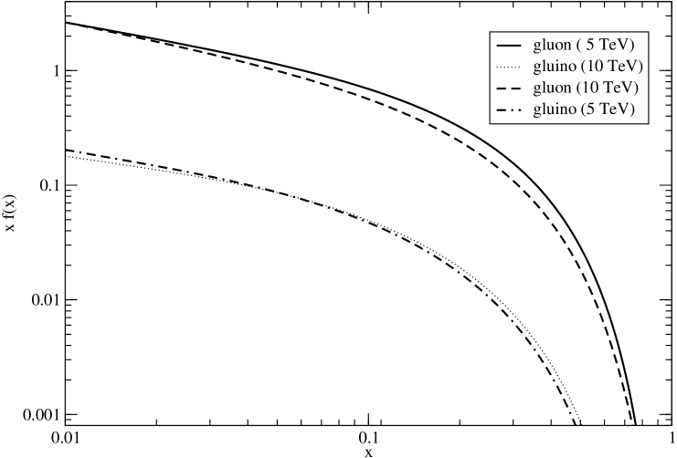We plot in fig. 8 the gluon and the gluino distributions for very large evolution scales for a realistic gluino mass of 250 GeV and varying factorization scales. We have chosen $Q_{f}=5$ and 10 TeV respectively. 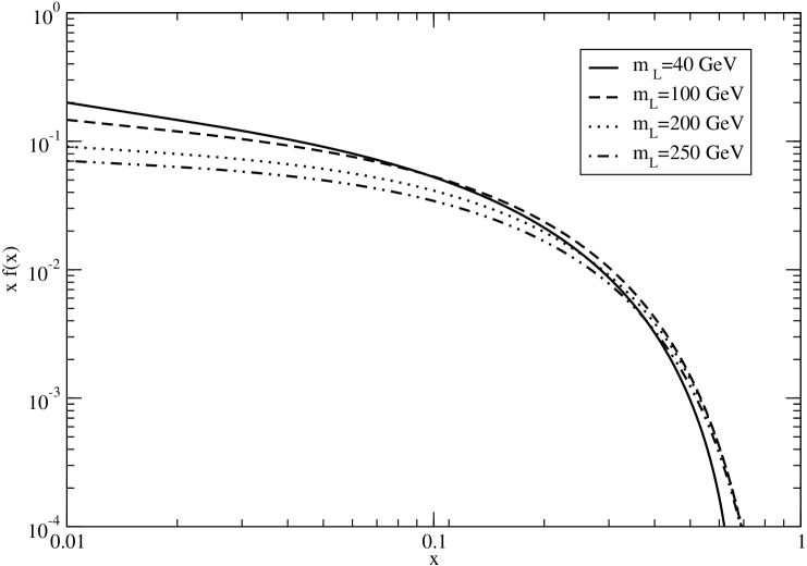The dependence on the final scale appears to be quite mild. Fig. 9 shows the variation of the gluino distribution for different gluino masses (40,100,200 and 250 GeV) and a fixed final evolution scale $Q_{f}=1$ TeV. 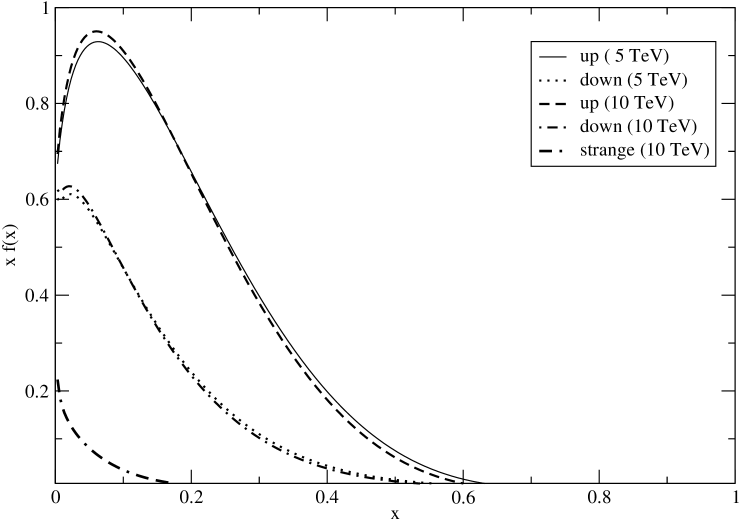There is a reduction of the small-x growth of this distribution at smaller-x values as the mass of the gluino is raised. In fig. 10 we show the dependence of all the quark distributions on the factorization scale $Q_{f}=5$ and 10 TeV in the case of a supersymmetric scale $m_{2\lambda}$ of 250 GeV.

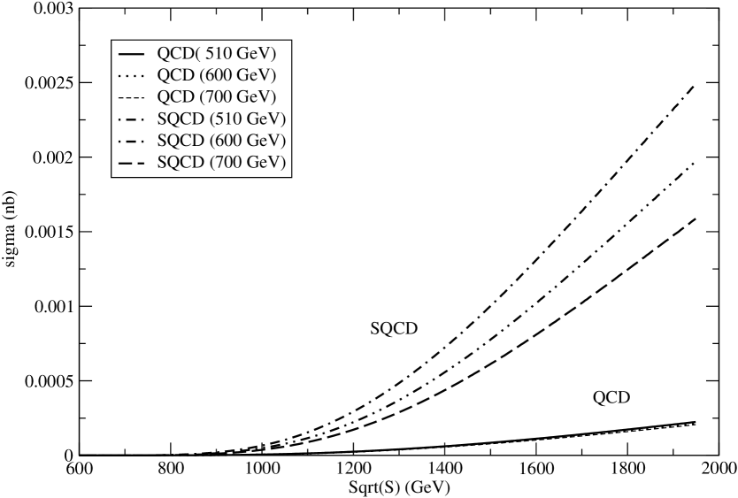
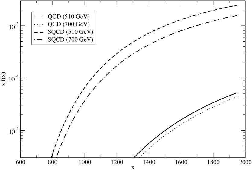
We study the impact of these corrections on future collider experiments by showing results for the 2-gluino production in a p-p collision. As can be seen from fig. 11, the production cross section is quite small -compared to standard QCD rates-, but gets enhanced by the inclusion of susy scaling violations especially at larger energies. We have set the gluino mass at 250 GeV. In the same figure we show the dependence of the cross section on the factorization scale (510,600 and 700 GeV). The dependence is sizeable, although the total rates remain small compared to the QCD background at these energies ( 650 GeV - 2 TeV). 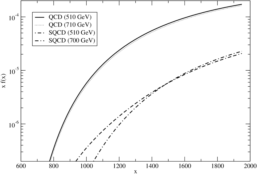We have shown in figs. 12 and 13 the partial contributions to fig. 11 coming from the $g\,g\to\lambda\lambda$ channel and the $q\,\bar{q}$ channel. The gluon contribution is the dominant part in both the regular QCD case and in the supersymmetric case.

9 Conclusions

We have solved the supersymmetric DGLAP equation in a scenario with a coupled gluino and a decoupled squark using an algorithm based on x-space. In particular, we have illustrated the evolution of the distributions of quarks and gluons and their supersymmetric versions using a radiative model. Although the window on a light gluino is now rapidly closing and the hope to detect supersymmetry from scaling violations in the initial state at the LHC with a light gluino is slim, the possibility of analizing experimentally the impact of heavier supersymmetric particles in the initial state remains, however, an important issue. In a specific example (p-p $\to\lambda\lambda$), we have seen that the total cross section is sensitive to initial state susy scaling violations and on the factorization scale chosen. For 2-gluino production, for instance, the rate is small, much below the usual QCD background, but gets sizeably enhanced when susy is included. Would be interesting to see how much we can rise the gluino mass and still obtain a signal on a final state which can not be compensated by the usual re-adjustement of the several parameters that describe the ordinary QCD parton distributions, or is comparable to it. In particular, the strong factorization scale dependence may be reduced by the inclusion of radiative corrections in the initial state. This and other related issues will be analized elsewhere.

Acknowledgements

I thank R. Pisarski and the Theory Group at Brookhaven National Laboratory and the C. N. Yang Institute for Theoretical Physics at Stony Brook for hospitality during the final stage of this investigation. I am grateful to R. Parwani, J. Smith, G. Sterman, J. Verbaarschot and A. Chuvakin at Stony Brook and to A. Stathopoulos of William Mary for discussions. This work is partially supported by MURST and by INFN (iniziativa specifica BARI-21).

9.1 Appendix 1: The Kernels

Various relations among different types of $``+^{\prime\prime}$ distributions can be derived. The kernels given in the literature may differ in their final expressions due to rearrangements of the corresponding “+” functions. We give here the expression of these kernels and illustrate some of the manipulations needed to reorganize them in a standard form.

In the derivation of the recursion relations we have used the identity

$$\int_{x}^{1}\frac{dy}{y}\left(\frac{1}{(1-x/y)_{+}}\right)A_{n}(y)=\int_{x}^{1}\frac{dy}{y}{yA_{n}(y)-xA_{n}(x)\over y-x}+\log(1-x)A_{n}(x)$$ (153)

Similarly, it is not hard to show the identity of the convolution products

$$\left({1+x^{2}\over 1-x}\right)_{+}\otimes A_{n}(x) = \int_{x}^{1}\frac{dy}{y}\frac{y^{2}+x^{2}}{(y-x)y}A_{n}(y)-A(x)\int_{0}^{x}dz\frac{1+z^{2}}{1-z}-A(x)\int_{x}^{1}\frac{dy}{y}\frac{y^{2}+x^{2}}{y^{2}(y-x)}$$

with

$$\left[\left({2\over(1-x)_{+}}\right)-1-x+\frac{3}{2}\delta(1-x)\right]\otimes A = \int_{x}^{1}\frac{dy}{y}2{yA_{n}(y)-xA_{n}(x)\over y-x}$$

$$- 2\log(1-x)A_{n}(x)+\frac{3}{2}A(x)-\int_{x}^{1}\frac{dy}{y}\left(1+z\right)A_{n}(y)$$

After some manipulations one can show that the two expressions given above are equal and therefore

$$\left({1+x^{2}\over 1-x}\right)_{+}={2\over(1-x)_{+}}-1-x+\frac{3}{2}\delta(1-x)$$ (156)

In leading order, the supersymmetric expression of the standard (qq,qg,gq,gg) QCD kernels are obtained by replacing $\alpha\to\alpha^{S}$, and the dependence on the coefficient of the $\beta$ function by its supersymmetric version $\beta_{0}\to\beta_{0}^{S}$.

The leading order expression of the kernels in the case of a decoupled scalar quark are given below. We have omitted the superscrit “S” for simplicity. We remark that the usual QCD kernels, after the embedding in the supersymmetric evolution, do not acquire new terms at $x=1$, except for $P_{gg}$.

$$P^{(0)\,}_{gg} = 2C_{A}\left[\frac{1}{(1-x)_{+}}+\frac{1}{x}-2+x(1-x)\right]+\frac{\beta_{0}^{S}}{2}\delta(1-x)$$

$$P^{(0)}_{g\lambda} = C_{\lambda}\left[\frac{1+(1-x)^{2}}{x}\right]$$

$$P^{(0)}_{gq} = P^{(0)}_{gq}=C_{F}\left[\frac{2}{x}-2+x\right]$$

$$P^{(0)}_{\lambda g} = n_{\lambda}\left[1-2x+2x^{2}\right]$$

$$P^{(0)}_{\lambda\lambda} = C_{\lambda}\left[\frac{2}{(1-x)_{+}}-1-x+\frac{3}{2}\delta(1-x)\right]=C_{\lambda}\left(\frac{1+x^{2}}{(1-x)}\right)_{+}$$

$$P^{(0)}_{\lambda\,\tilde{q}} = 0$$

$$P^{(0)}_{\tilde{q}\,\lambda} = 0$$

$$P^{(0)}_{\tilde{q}\,\tilde{q}} = 0$$

$$P^{(0)}_{\tilde{q}\,q} = 0$$

$$P^{(0)}_{q\,\tilde{q}} = 0$$

$$P^{(0)}_{qg} = P^{(0)}_{qg}=n_{f}\left[x^{2}+(1-x)^{2}\right]$$

$$P^{(0)}_{q\lambda} = n_{f}(1-x)$$

$$P^{(0)\,S}_{qq} = C_{F}\left[{(1+x^{2})\over(1-x)}\right]_{+}$$

$$= C_{F}\left({2\over(1-x)_{+}}-1-x+\frac{3}{2}\delta(1-x)\right)$$

10 Appendix 2. Discretizations

For the calculation of the weights used in the numerical analysis we follow closely ref. [6] also implemented in [7]. At each x-value, these authors use an approximation characterized by weights which are calculated analytically, together with an interpolation formula for the integration function. The method allows to monitor the singularity appearing in the small-x region and to achieve a very good numerical accuracy. The method speeds up in time the calculation by a large factor, but becomes tedious when moving to a higher order, since all the integrals have to be exactly discretized and the logarithms extracted in each sub-interval. Here we briefly illustrate the method as it applies to our case.

We briefly recall the numerical strategy employed in this analysis. We define $\bar{P}(x)\equiv xP(x)$ and $\bar{A}(x)\equiv xA(x)$. We also define the convolution product

$$J(x)\equiv\int_{x}^{1}\frac{dy}{y}\left(\frac{x}{y}\right)P\left(\frac{x}{y}\right)\bar{A}(y).\$$ (158)

The integration interval in $y$ at any fixed x-value is partitioned in an array of increasing points ordered from left to right $\left(x_{0},x_{1},x_{2},...,x_{n},x_{n+1}\right)$ with $x_{0}\equiv x$ and $x_{n+1}\equiv 1$ being the upper edge of the integration region. One constructs a rescaled array $\left(x,x/x_{n},...,x/x_{2},x/x_{1},1\right)$. We define $s_{i}\equiv x/x_{i}$, and $s_{n+1}=x<s_{n}<s_{n-1}<...s_{1}<s_{0}=1$. We get

$$J(x)=\sum_{i=0}^{N}\int_{x_{i}}^{x_{i+1}}\frac{dy}{y}\left(\frac{x}{y}\right)P\left(\frac{x}{y}\right)\bar{A}(y)$$ (159)

At this point we introduce the linear interpolation

$$\bar{A}(y)=\left(1-\frac{y-x_{i}}{x_{i+1}-x_{i}}\right)\bar{A}(x_{i})+\frac{y-x_{i}}{x_{i+1}-x_{i}}\bar{A}(x_{i+1})$$ (160)

and perform the integration on each subinterval with a change of variable $y->x/y$ and replace the integral $J(x)$ with its discrete approximation $J_{N}(x)$ to get

$$J_{N}(x) = \bar{A}(x_{0})\frac{1}{1-s_{1}}\int_{s_{1}}^{1}\frac{dy}{y}P(y)(y-s_{1})$$

$$+ \sum_{i=1}^{N}\bar{A}(x_{i})\frac{s_{i}}{s_{i}-s_{i+1}}\int_{s_{i+1}}^{s_{i}}\frac{dy}{y}P(y)(y-s_{i+1})$$

$$- \sum_{i=1}^{N}\bar{A}(x_{i})\frac{s_{i}}{s_{i-1}-s_{i}}\int_{s_{i}}^{s_{i-1}}\frac{dy}{y}P(y)(y-s_{i-1}).$$

Introducing the coefficients $W(x,x)$ and $W(x_{i},x)$, the integral is cast in the form

$$J_{N}(x)=W(x,x)\bar{A}(x)+\sum_{i=1}^{n}W(x_{i},x)\bar{A}(x_{i})$$ (162)

where

$$W(x,x) = \frac{1}{1-s_{1}}\int_{s_{1}}^{1}\frac{dy}{y}(y-s_{1})P(y),$$

$$W(x_{i},x) = \frac{s_{i}}{s_{i}-s_{i+1}}\int_{s_{i+1}}^{s_{i}}\frac{dy}{y}\left(y-s_{i+1}\right)P(y)$$

$$- \frac{s_{i}}{s_{i-1}-s_{i}}\int_{s_{i}}^{s_{i-1}}\frac{dy}{y}\left(y-s_{i-1}\right)P(y).$$

We recall that

$$\int_{0}^{1}dx\frac{f(x)}{(1-x)_{+}}=\int_{0}^{1}{dy}\frac{f(y)-f(1)}{1-y}$$ (164)

and that

$$\frac{1}{(1-x)_{+}}\otimes f(x)\equiv\int_{x}^{1}\frac{dy}{y}\frac{\,\,yf(y)-xf(x)}{y-x}+f(x)\log(1-x)$$ (165)

as can can be shown quite straightforwardly.

We also introduce the expressions

$$In_{0}(x) = \frac{s_{1}}{1-s_{1}}\log(s_{1})+\log(1-s_{1})$$

$$Jn_{i}(x) = \frac{1}{s_{i}-s_{i+1}}\left[\log\left(\frac{1-s_{i+1}}{1-s_{i}}\right)+s_{i+1}\log\left(\frac{1-s_{i}}{1-s_{i+1}}\frac{s_{i+1}}{s_{i}}\right)\right]$$

$$Jnt_{i}(x) = \frac{1}{s_{i-1}-s_{i}}\left[\log\left(\frac{1-s_{i}}{1-s_{i-1}}\right)+s_{i-1}\log\left(\frac{s_{i}}{s_{i-1}}\right)+s_{i-1}\left(\frac{1-s_{i-1}}{1-s_{i}}\right)\right],\,\,\,\,\,\ i=2,3,..N$$

$$Jnt_{1}(x) = \frac{1}{1-s_{1}}\log s_{1}.$$

Using the linear interpolation formula (160) we get the relation

$$\int_{x}^{1}\frac{dy}{y}\frac{yA_{n}(y)-xA_{n}(x)}{y-x} = -\log(1-x)A_{n}(x)+A_{n}(x)In_{0}(x)$$ (167)

$$+\sum_{i=1}^{N}A_{n}(x_{i})\left(Jn_{i}(x)-Jnt_{i}(x)\right)$$

which has been used for a fast and accurate numerical implementation of the recursion relations.

Figure 1: u, d, s and gluon distributions at $Q_{i}=5$ GeV

Figure 2: $xu(x)$ and $xd(x)$ evaluated with $Q_{i}=2.0$ GeV and $Q_{f}=100$ GeV with $m_{\lambda}=10$ GeV in the standard (reg) and susy evolution

Figure 3: Gluon distributions with $Q_{i}=2.0$ GeV and $Q_{f}=100$ GeV with intermediate $m_{\lambda}=10$ GeV. The regular and the susy evolution are shown

Figure 4: $xq^{(+)}(x)$ (singlet) quark distribution evaluated with $Q_{i}=5.0$ GeV and $Q_{f}=100$ GeV with $m_{\lambda}=10$ GeV in the standard (non-susy) and susy evolution

Figure 5: Comparison of the supersymmetric gluon and gluino distributions for $m_{\lambda}=30$ GeV and $Q_{f}=100$ GeV.

Figure 6: Gluon distribution for 3 values of the gluino mass 100, 150 and 200 GeV and a final evolution scale $Q_{f}=1$ TeV. Shown is also the regular (reg) evolution of the same distribution

Figure 7: Gluino distribution for $Q_{f}=1,2$ and 5 TeV and $m_{\lambda}=100$ GeV

Figure 8: Gluino and gluon distributions for very large final evolution scales $Q_{f}=5$ and 10 TeV. The gluino mass is 250 GeV

Figure 9: Gluino distributions for a varying $m_{\lambda}$ (40, 100, 200 and 250 GeV) with a fixed final evolution scale $Q_{f}=1$ TeV.

Figure 10: u, d quark distributions $m_{\lambda}=250$ GeV with a varying final evolution scale $Q_{f}=5$ and 10 TeV. Shown is also the strange quark distribution with $Q_{f}=5$ TeV.

Figure 11: Dependence of the total 2-gluino cross section $\sigma_{pp\to\lambda\lambda}$ on the factorization scale in the QCD and SQCD cases ($m_{\lambda}=250$ GeV). Shown are the factorization scales $Q_{fact}$= 510, 600 and 700 GeV. We show both the QCD and the SQCD results

Figure 12: Dependence of the total 2-gluino cross section $\sigma_{gg\to\lambda\lambda}$ on the factorization scale in the QCD and SQCD cases ($m_{\lambda}=250$ GeV). Shown are the factorization scales $Q_{fact}$= 510 and 700 GeV.We show both the QCD and the SQCD results.

Figure 13: Dependence of the total 2-gluino cross section $\sigma_{q\bar{q}\to\lambda\lambda}$ on the factorization scale in the QCD and SQCD cases ($m_{\lambda}=250$ GeV). Shown are the factorization scales $Q_{fact}$= 510 and 700 GeV.We show both the QCD and the SQCD results.