LBNL-46831

UCB-PTH-00/29

hep-ph/0009174

September 2000

Anarchy and Hierarchy
Naoyuki Haba

Faculty of Engineering, Mie University
Tsu, Mie, 514-8507, Japan
Hitoshi Murayama

Department of Physics, University of California
Berkeley, CA  94720, USA
and
Theory Group, Lawrence Berkeley National Laboratory
Berkeley, CA  94720, USA

We advocate a new approach to study models of fermion masses and mixings, namely anarchy proposed in Ref. [1]. In this approach, we scan the $O(1)$ coefficients randomly. We argue that this is the correct approach when the fundamental theory is sufficiently complicated. Assuming there is no physical distinction among three generations of neutrinos, the probability distributions in MNS mixing angles can be predicted independent of the choice of the measure. This is because the mixing angles are distributed according to the Haar measure of the Lie groups whose elements diagonalize the mass matrices. The near-maximal mixings, as observed in the atmospheric neutrino data and as required in the LMA solution to the solar neutrino problem, are highly probable. A small hierarchy between the $\Delta m^{2}$ for the atmospheric and the solar neutrinos is obtained very easily; the complex seesaw case gives a hierarchy of a factor of 20 as the most probable one, even though this conclusion is more measure-dependent. $U_{e3}$ has to be just below the current limit from the CHOOZ experiment. The CP-violating parameter $\sin\delta$ is preferred to be maximal. We present a simple $SU(5)$-like extension of anarchy to the charged-lepton and quark sectors which works well phenomenologically.

1 Introduction

The seemingly useless repetition of families has been a big puzzle in particle physics since the discovery of the muon. Even more puzzling has been the fact that the particles in three families, despite their exactly the same gauge quantum numbers, have hierarchical masses and small mixing angles. It appears, however, that we have lost the sense of the initial surprise having been accustomed to hierarchical masses and small mixings. The very reason of the puzzle was the following simple naive expectation: the quantum mechanical states with the same quantum numbers are likely to have similar energies and should mix significantly. Having tried to explain the hierarchy and small mixing angles for decades, we seem to have forgotten what the naive expectation was.

There was a revolution when the top quark was finally discovered. We were used to the idea that the weak gauge bosons are “heavy” while the quarks, leptons are “light.” During the search for the top quark for almost two decades, we used to question why the top quark is so heavy, i.e., beyond the reach of the experiments. After the discovery of the top quark, however, we realized that the top quark has the most natural mass among all quarks and leptons because its Yukawa coupling to the Higgs boson condensate is $h_{t}=1.0$ similarly to the gauge coupling constants $e=0.3$, $g=0.8$, $g_{s}=1.2$. Now we think that the puzzle is not why the top quark is heavy, but rather why all the other quarks and leptons are light.

In our opinion, the near-maximal mixing in the atmospheric neutrino data from the SuperKamiokande experiment is another revolution of the same kind as the case with the top quark. It simply demands us to go back to the naive expectation: unless there are definite quantum numbers for three neutrino flavor states to be distinguished, they should fully mix and have comparable masses. We are proposing this simple change in the perspective. One may suspect, however, that this naive expectation would not lead to the apparent “maximal mixing” nor the hierarchy between two $\Delta m^{2}$ values required to explain atmospheric and solar neutrino data. It was pointed out that a seesaw mass matrix without a particular structure should appear random from the low-energy point of view (anarchy), and a random matrix can well account for the observed pattern of neutrino mass and mixings [1].

Therefore, it appears phenomenologically viable to consider all mass matrix elements for neutrinos within the seesaw mechanism for small neutrinos to be $O(1)$ without a particular structure: anarchy. However, one should ask if any of the results based on this idea would depend on the particular choice of the measure. We show that the key requirement is that the measure should not depend on the choice of the basis with which the matrix elements are defined. Once this requirement of basis-independence is made, distributions over the mixing angles are determined by the invariant Haar measure of the diagonalization matrices as we will see in Section 3.

We first present the concept of anarchy in Section 2. We argue that the anarchy is an alternative approach to traditional model building which is applicable to wider range of theories. In Section 3, we show how the distributions in the MNS mixing angles can be obtained from anarchy. The assumed lack of fundamental distinction among three generations of neutrinos implies that the basis-independence of the measure. Then the distributions in mixing angles are obtained solely by the Haar measure of the group which diagonalizes the mass matrices. The predicted distributions are contrasted to the experimental data in Section 4. Anarchy, however, raises another question: why the charged leptons, down quarks, and especially up quarks have hierarchical masses and small mixings. We introduce a simple approximate $U(1)$ flavor symmetry which can answer this question in Section 5. In Section 6, we conclude.

2 Anarchy

The idea of anarchy is simple: all coefficients of operators which do not have particular reasons to be small, i.e., allowed by symmetries of the theory, are $O(1)$, and do not have particular pattern, i.e., appear random from the low-energy point of view. A fundamental theory should determine the $O(1)$ constants, but if it is sufficiently complex, the $O(1)$ constants indeed likely appear random. Even though it is difficult to quantify the “random”ness of the $O(1)$ constants, what should appear random are the parameters in the Lagrangian, such as Yukawa matrix elements, rather than the physical observables such as masses and mixing angles which are defined only after diagonalization of matrices in the Lagrangian. Therefore, we take the point of view that the individual elements of the Yukawa or mass matrices are distributed randomly.

The idea of random $O(1)$ constants is used commonly in many different contexts. For instance, in the chiral Lagrangian description of the low-energy hadron physics, one often faces the situation that one cannot predict the coefficient of the operators in the chiral Lagrangian from the corresponding operator written in terms of quarks and gluon fields. Even though there should be in principle one-to-one correspondence between the Wilson coefficient in the QCD and the coefficient of chiral Lagrangian operators, it is beyond the scope of current techniques. In this kind of situation, one often revokes the “naive dimensional analysis” where one assumes an $O(1)$ coefficient unless there is a symmetry reason that the coefficient is suppressed. For instance, if two chiral Lagrangian operators contribute to a single process at the same order, people often argue that there should not be any severe cancellations between two contributions unless there is a reason for it. Similar situation arises, for instance, if some of the particles in the Standard Model are actually composite. From the point of view of the low-energy effective theory, the couplings are all $O(1)$ without a particular pattern: random.

In most compactifications of the superstring theory, Yukawa couplings among light degrees of freedom are $O(1)$, sometimes zero. It is quite unusual to have small Yukawa couplings such as $10^{-6}$ for the electron whenever there is no reason that they are suppressed. From the point of view of the low-energy effective field theory, the $O(1)$ couplings do not seem to have any particular pattern: random.

In grand-unified theories (GUTs) or Froggatt–Nielsen models of flavor, one introduces (quite a few) vector-like particles which become massive at a certain energy scale and decouple. Even if all coupling constants are very close to unity, the low-energy coupling constants depend on many coupling constants, many VEVs and many inverse masses, and small deviations of coupling constants from unity get amplified. In the end we expect that the low-energy coupling constants are somewhat randomly distributed around unity. Even the famous “prediction” of the $SU(5)$ grand-unification $m_{D}=m_{L}^{T}$, where $m_{D}$ and $m_{L}$ are down-quark and charged-lepton Dirac mass matrices, is likely to be spoiled by the mixing of many vector-like particles at the GUT-scale picking the GUT-breaking VEVs. In the limit of large number of vector-like particles mixed with each other, the low-energy coupling constants become completely randomized.

In all of the above examples, seemingly random $O(1)$ coefficients arise in the low-energy effective theories as a consequence of the lack of precise knowledge on the fundamental theory. Once the dynamics of the fundamental theory is completely understood, which we hope to do with the lattice QCD on the first example, the seemingly random $O(1)$ numbers can be predicted. Still, in the absence of a fundamental theory behind the fermion masses and mixings, as opposed to the case of the hadronic physics where we know that the QCD is the fundamental theory, we should attempt to obtain some quantitative results without relying on the details of the dynamics.

We know of a perfectly sensible and beautiful theory of this kind: statistical mechanics. When studying a collection of an astronomical number of particles, e.g., Avogadro number, it is hopeless to measure the positions and the momenta of each particle precisely to predict the configuration of the particles in the future, even in the deterministic classical mechanics. However the large number of particles allow us to believe that the motion of particles is completely randomized under various symmetry requirements, such as conservation of charges, number of particles, energy, etc, at least on average. We can draw quantitative conclusions out of the randomness on the statistical basis. We cannot predict the precise configuration of particles at a given instance. However, we can predict the distributions in momenta, energies, positions, etc, with confidence.

What we advocate is a similar statistical treatment on the seemingly random $O(1)$ coefficients in low-energy effective theories consistent with certain symmetry requirements. We scan over the $O(1)$ coefficients randomly. However, an important question that arises here is what measure to use for the random scan. In the case of statistical mechanics, Boltzmann distribution is justified as a consequence of the interaction between the relevant system with the infinitely large heat reservoir. In our case, the choice of a particular distribution appears unwarranted. Nonetheless, one may obtain distributions out of the random scan over the $O(1)$ parameters which do not depend on the choice of a particular measure; then such distributions can be regarded as rigorous predictions of the anarchy. As we will see below, the mixing matrices among neutrinos can be predicted from the anarchy and be compared to the experimental situations.

The anarchy is a complimentary approach to the traditional model building. Traditionally, one attempts to write down a complete model of flavor by imposing certain symmetry which (hopefully) forbids all unwanted operators while explaining the observed structure of masses and mixings. We would call this “monarchy” approach, as one aims for a model which is constrained tightly by the symmetries imposed and the particle content assumed with little freedom so that the model is predictive. Then one hopes that the nature chose that particular model. The advantage of this approach is that the model is predictive by design. The disadvantage is that the model tends to become rather contrived and is not necessarily be believable. The whole idea is based on the optimism that the high-energy physics is rather simple so that we can (eventually) test it directly from the low-energy observables. The anarchy is the opposite approach. We impose as little as possible. Based on the statistical method, we try to figure out the tendency of the consequences from a given framework on the low-energy physics. This approach is certainly not predictive, while it can be powerful enough so that it is applicable even in the situation where the high-energy physics is extremely complicated. This way, we can test if a certain simple idea is viable or not without going into details of particular models.

3 Anarchy of Neutrinos

In this section, we apply the anarchy approach to the neutrino mass matrices. The fundamental assumption of our analysis is that there is no physical distinction among three generation of lepton doublets. We would like to test this assumption by working out its consequences using the statistical method as discussed in the previous section. The key requirement is that the measure should not depend on the choice of the basis with which the matrix elements are defined because there is no physical distinction among three generations by assumption. Once this requirement of basis-independence is made, distributions over the mixing angles are determined by the invariant Haar measure of the diagonalization matrices.

3.1 A Simple Two-by-two Case

It is instructive to study the consequence of a simple two-by-two Majorana mass matrix for neutrinos assuming that each independent matrix element is distributed randomly. Since a Majorana mass matrix is a symmetric matrix, there are only three parameters

$$M_{\nu}=\left(\begin{array}[]{cc}M_{11}&M_{12}\\ M_{12}&M_{22}\end{array}\right),$$ (1)

and we assume the matrix elements to be real for simplicity of the discussion. One can rewrite this matrix in terms of physical observables,

$$M_{\nu}=m_{\rm average}+\frac{\Delta m}{2}\left(\begin{array}[]{cc}-\cos 2\theta&\sin 2\theta\\ \sin 2\theta&\cos 2\theta\end{array}\right).$$ (2)

Based on the assumption that the matrix elements $M_{11}$, $M_{12}$, $M_{22}$ are distributed randomly, we can qualitatively understand how the mixing angle is distributed. By rewriting the volume element $dM_{11}\wedge dM_{12}\wedge dM_{22}$ in terms of the observables, we find

$$dM_{11}\wedge dM_{12}\wedge dM_{22}=\Delta mdm_{\rm average}\wedge d(\Delta m)\wedge d\theta,$$ (3)

and the volume is flat write respect to the mixing angle. (We will omit the wedge symbol below.) Then the distribution in $\sin^{2}2\theta$ is naturally peaked at zero and the maximal angles,

$$d\theta=\frac{1}{4\cos 2\theta\sin 2\theta}d(\sin^{2}2\theta).$$ (4)

Note that the measure $d\theta$ over the angle is the invariant Haar measure of the $U(1)$ group.

In the realistic situation, we should consider a complex matrix. As suggested by the phenomenological success of Kobayashi–Maskawa theory of CP violation, Nature appears to have chosen complex Yukawa matrices. Then all the three independent elements of the matrix Eq. (1) are complex. Correspondingly, the diagonalization matrix is unitary. It can always be diagonalized by a unitarity matrix $U$,

$$M_{\nu}=U\left(\begin{array}[]{cc}m_{1}&0\\ 0&m_{2}\end{array}\right)U^{T},$$ (5)

where the unitarity matrix $U$ can be parameterized as

$$U=e^{i\eta}\left(\begin{array}[]{cc}e^{i\omega}&0\\ 0&e^{-i\omega}\end{array}\right)\left(\begin{array}[]{cc}\cos\theta&\sin\theta\\ -\sin\theta&\cos\theta\end{array}\right)\left(\begin{array}[]{cc}e^{i\phi}&0\\ 0&e^{-i\phi}\end{array}\right).$$ (6)

We chose this parameterization such that the angles $\eta$ and $\omega$ are unphysical. They can be absorbed by rephasing into the definition of the flavor and mass eigenstates. The angle $\phi$ is a CP-violating phase, even though it does not appear in neutrino oscillation for this two-flavor case. The measure for the matrix elements can then be rewritten as

$$d^{2}M_{11}d^{2}M_{12}d^{2}M_{22}=(m_{2}^{2}-m_{1}^{2})dm_{1}^{2}dm_{2}^{2}dU,$$ (7)

where the measure over the angles is the invariant Haar measure over the $U(2)$ group

$$dU=d(\sin^{2}\theta)d\eta d\omega d\phi$$ (8)

up to a normalization constant. Note that the distribution in $\theta$ is peaked even more strongly at the maximal mixing

$$d(\sin^{2}\theta)=2\sin\theta\cos\theta d\theta=\frac{1}{4\cos 2\theta}d(\sin^{2}2\theta).$$ (9)

We therefore conclude that a mass matrix without a particular structure would lead to a near-maximal mixing quite “often.” This observation should be contrasted to the wide-spread perception that a near-maximal mixing in the atmospheric neutrino data is very special.

3.2 Why Haar Measure?

In general, the measure over the angles are given solely in terms of the invariant Haar measure over the relevant group. This is true as long as that the measure does not depend on the basis with which the matrix elements are defined. The proof is very simple. Since we discuss seemingly random mass matrix of neutrinos here, the measure with which we scan the parameter space should not depend on a particular choice of the basis of neutrino states. This is the central assumption of basis-independence. The measure discussed above for the two-flavor case, linear w.r.t. the individual mass matrix elements, satisfies this property, because the change of basis transforms the elements homogeneously as a unitarity rotation. In fact, one can show that the distributions are determined by the invariant Haar measure over the relevant group from the requirement of the basis-independence. This observation allows us to separate the measure over the mass matrix elements in terms of eigenvalues and group transformations.

Taking the complex Majorana case as an example, any mass matrix can be written as

$$M=UDU^{T},$$ (10)

where $U\in U(N)$ and $D=\mbox{diag}(m_{1},m_{2},\cdots,m_{N})$ is a real diagonal matrix. Because of the invariance of the measure $dM$ under the change of basis $M\rightarrow VMV^{T}$, the measure $dM$ should contain the measure over the group $dU$ which is invariant under the left translation $U\rightarrow VU$. Since $U(N)$ is a compact Lie group, a left-invariant measure is also right-invariant. Therefore, $dU$ should be the invariant Haar measure over the group $U(N)$. Then the measure $dM$ can be written as

$$dM=f(m_{1},\cdots,m_{N})\prod_{i=1}^{N}dm_{i}dU.$$ (11)

Here the yet-undetermined function $f$ is symmetric under the interchange of eigenvalues. In the appendix it is shown that the weight function $f$ should contain the factor $\prod_{i<j}(m_{i}^{2}-m_{j}^{2})\prod_{i}m_{i}$, and for the case of the linear measure, this exhausts the weight function $f$. The only possible change of the measure is to introduce a weight function which depends on invariants, such as ${\rm Tr}M^{\dagger}M$, ${\rm det}M$. However, such weight functions can depend only on the eigenvalues of the mass matrix, consistent with the basis-independence. Therefore the measure over the angles obtained from the Haar measure cannot be changed by the choice of the measure, and hence the distributions of the angle above are predictions of anarchy. Exactly the same argument goes through for the Dirac and seesaw mass matrices.

Of course one should consider the diagonalization of the charged lepton mass matrix we well, since the MNS matrix is the mismatch between two diagonalization matrices, one of the neutrinos and the other of the charged leptons. However, the translational invariance of the Haar measure guarantees that the diagonalization of the charged lepton mass matrix can be absorbed into the Haar measure and hence the Haar measure gives the distributions of the MNS angles. We consider a random scan over both the neutrino mass and the charged lepton mass matrices. For a particular pick of the charged lepton mass matrix $M_{l}=U_{l}D_{l}U_{e}^{-1}$, we still scan over the neutrino mass matrix $M_{\nu}=U_{\nu}D_{\nu}U_{\nu}^{T}$, which we assume to be a complex Majorana matrix again for definiteness. The measure is given in general by

$$dM_{l}dM_{\nu}=f(m_{l_{i}},U_{e})g(m_{\nu_{i}})dm_{l_{i}}dm_{\nu_{i}}dU_{l}dU_{e}dU_{\nu}.$$ (12)

The basis-independence is imposed only on left-handed lepton doublets, and hence the measure may depend non-trivially on $U_{e}$. However, $U_{e}$ is an unobservable matrix. We can integrate over $U_{e}$ and obtain an effective weight factor

$$\tilde{f}(m_{l_{i}})=\int dU_{e}f(m_{l_{i}},U_{e}).$$ (13)

Now we can use $U_{MNS}=U_{l}^{-1}U_{\nu}$ instead of $U_{\nu}$, and the translational invariance of the Haar measure guarantees that $dU_{l}dU_{e}dU_{\nu}=dU_{l}dU_{e}dU_{MNS}$, where $U_{l}$ is now unobservable and its measure can be dropped. The measure simplifies to

$$dM_{l}dM_{\nu}=\tilde{f}(m_{l_{i}})g(m_{\nu_{i}})dm_{l_{i}}dm_{\nu_{i}}dU_{MNS}.$$ (14)

Therefore, the distributions for the MNS mixing angles and the CP-violating phases are predicted in terms of the Haar measure again. The only implicit assumption made in this argument is that the scan over the charged lepton and neutrino mass matrices are uncorrelated. We believe this is a natural consequence of typical flavor models as the mass matrices of the fields with different gauge quantum numbers are generated independently from different chain of the Froggatt–Nielsen fields, for example.

Because of this, distributions in the mixing angles are direct consequences of the group structure and do not depend on the details of how one defines the measure. On the other hand, the measure for the eigenvalues can depend on the details because one can modify the weight factor $f(m_{i})$ which is a symmetric function of all eigenvalues without affecting the basis-independence of the measure.

3.3 Three-by-Three case

For three generation case, details are discussed in Appendix A. Here we merely summarize the results. We decompose the linear measure over the real or complex elements of both Majorana and Dirac mass matrices into the measure over the angles and the mass eigenvalues.

For the real Majorana case, the symmetric real mass matrix is written as $M=ODO^{T}$ where $O$ is an $SO(3)$ diagonalization matrix and $D={\rm diag}(m_{1},m_{2},m_{3})$. Then we find

$$dM=(m_{1}-m_{2})(m_{2}-m_{3})(m_{3}-m_{1})dm_{1}dm_{2}dm_{3}dO,$$ (15)

where $dO$ is the invariant Haar measure of the $SO(3)$ group.

For the real Dirac case, the mass matrix is written as $M=O_{L}DO_{R}^{T}$ where $O_{L,R}$ are $SO(3)$ diagonalization matrices and $D={\rm diag}(m_{1},m_{2},m_{3})$. Then we find

$$dM=(m_{1}^{2}-m_{2}^{2})(m_{2}^{2}-m_{3}^{2})(m_{3}^{2}-m_{1}^{2})dm_{1}dm_{2}dm_{3}dO_{L}dO_{R}.$$ (16)

Again $dO_{L}$, $dO_{R}$ are invariant Haar measures for the corresponding $SO(3)$ groups.

For the complex Majorana case, the mass matrix is written as $M=UDU^{T}$ where $U$ is a $U(3)$ diagonalization matrix and $D={\rm diag}(m_{1},m_{2},m_{3})$. Then we find

$$dM=(m_{1}^{2}-m_{2}^{2})(m_{2}^{2}-m_{3}^{2})(m_{3}^{2}-m_{1}^{2})m_{1}m_{2}m_{3}dm_{1}dm_{2}dm_{3}dU,$$ (17)

where $dU$ is the invariant Haar measure of the $U(3)$ group.

For the complex Dirac case, the mass matrix is written as $M=U_{L}DU_{R}^{\dagger}$ where $U_{L,R}$ are $U(3)$ diagonalization matrices and $D={\rm diag}(m_{1},m_{2},m_{3})$. Then we find

$$dM=(m_{1}^{2}-m_{2}^{2})^{2}(m_{2}^{2}-m_{3}^{2})^{2}(m_{3}^{2}-m_{1}^{2})^{2}m_{1}m_{2}m_{3}dm_{1}dm_{2}dm_{3}\frac{dU_{L}dU_{R}}{d\varphi_{1}d\varphi_{2}d\varphi_{3}}.$$ (18)

Because of the reparameterization invariance $U_{L}\rightarrow U_{L}\Phi$, $U_{R}\rightarrow U_{R}\Phi$, with $\Phi={\rm diag}(e^{i\varphi_{1}},e^{i\varphi_{2}},e^{i\varphi_{3}})$, the Haar measure $dU_{L}dU_{R}$ is modded out by this invariance.

Finally, we consider also seesaw neutrino mass matrices, which are arguably the most promising ones in order to explain the smallness of neutrino masses as well as the most motivated one from the point of view of grand unification. In this case, we have Majorana-type right-handed neutrino mass matrix $M_{R}$ as well as Dirac-type mass matrix between left- and right-handed neutrinos $M_{D}$. The full mass matrix is given by

$$\left(\begin{array}[]{cc}0&M_{D}\\ M_{D}^{T}&M_{R}\end{array}\right),$$ (19)

such that the full Majorana-type mass matrix is symmetric. It is assumed that there is a large hierarchy between the eigenvalues of $M_{D}$ to those of $M_{R}$. The mass matrix among the heavy (dominantly right-handed) neutrino states is just $M_{R}$ up to corrections of the order of $M_{D}^{2}/M_{R}^{2}$, while that among the light (dominantly left-handed) neutrino states is given by

$$M_{D}M_{R}^{-1}M_{D}^{T},$$ (20)

again up to corrections of the order of $M_{D}^{2}/M_{R}^{2}$. This is the famous seesaw formula. Hereafter we discuss only the complex case. By diagonalizing both $M_{D}=U_{L}D_{D}U_{R}^{-1}$ with $D_{D}={\rm diag}(m_{1},m_{2},m_{3})$ and $M_{R}=U_{M}D_{M}U_{M}^{T}$ with $D_{M}={\rm diag}(M_{1},M_{2},M_{3})$, we find the linear measure to be

$$dM_{D}dM_{R}=$$ (21)

$$(m_{1}^{2}-m_{2}^{2})^{2}(m_{2}^{2}-m_{3}^{2})^{2}(m_{3}^{2}-m_{1}^{2})^{2}m_{1}m_{2}m_{3}dm_{1}dm_{2}dm_{3}\frac{dU_{L}dU_{R}}{d\varphi_{1}d\varphi_{2}d\varphi_{3}}$$

$$(M_{1}^{2}-M_{2}^{2})(M_{2}^{2}-M_{3}^{2})(M_{3}^{2}-M_{1}^{2})M_{1}M_{2}M_{3}dM_{1}dM_{2}dM_{3}dU_{M}.$$

However, the light neutrino mass matrix is then given by $U_{L}D_{D}U_{R}^{-1}U_{M}D_{M}^{-1}U_{M}^{T}U_{R}^{-1T}D_{D}U_{L}^{T}$, and hence $U_{R}$ and $U_{M}$ are not separately physical but only the combination $U_{\rm rel}=U_{R}^{-1}U_{M}$. Therefore one can simplify the measure $dU_{R}dU_{M}$ to just $dU_{\rm rel}$. Note that one still needs to diagonalize the matrix

$$\left(\begin{array}[]{ccc}m_{1}&&\\ &m_{2}&\\ &&m_{3}\end{array}\right)U_{rel}\left(\begin{array}[]{ccc}M_{1}^{-1}&&\\ &M_{2}^{-1}&\\ &&M_{3}^{-1}\end{array}\right)U_{rel}^{-1T}\left(\begin{array}[]{ccc}m_{1}&&\\ &m_{2}&\\ &&m_{3}\end{array}\right)$$ (22)

to find the mass eigenvalues of the light neutrinos. On the other hand, the measure $dU_{L}$ can be replaced by $dU_{MNS}$ as discussed earlier.

In each of the cases, we find that the distributions in the MNS mixing angles are determined solely by the Haar measure.

3.4 Distributions in Angles

Now that we have learned that the distributions in the MNS mixing angles are distributed according to the Haar measure, we would like to see how they look. The distributions are different for the $SO(3)$ case (real mass matrices) and the $U(3)$ case (complex mass matrices).

First for the case of real matrices, the distributions in the MNS mixing angles are given in terms of the $SO(3)$ Haar measure (see Appendix A.2)

$$dO=\cos\theta_{13}d\theta_{12}d\theta_{13}d\theta_{23}.$$ (23)

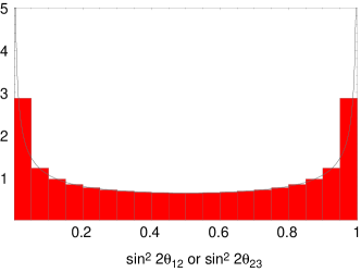
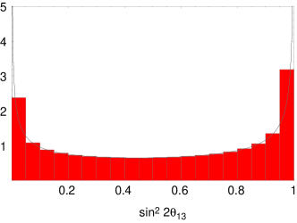
It is straightforward to plot the distributions against $\sin^{2}2\theta_{ij}$. In Fig. 1, we show distributions in (a) $\sin^{2}2\theta_{12}$ or $\sin^{2}2\theta_{23}$, and (b) $\sin^{2}2\theta_{13}$. The solid lines show the differential distributions and the histograms the integrated probabilities with the bin size of $0.05$.

Figure 1: Distributions in (a) $\sin^{2}2\theta_{12}$ or $\sin^{2}2\theta_{13}$ and (b) $\sin^{2}2\theta_{13}$ for the case of real mass matrices.

Second for the realistic case of complex matrices, the distributions in the MNS mixing angles are given in terms of the $U(3)$ Haar measure (see Appendix A.2)

$$dU=ds_{12}^{2}dc_{13}^{4}ds_{23}^{2}d\delta d\eta d\phi_{1}d\phi_{2}d\chi_{1}d\chi_{2}.$$ (24)

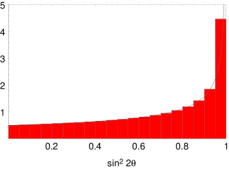
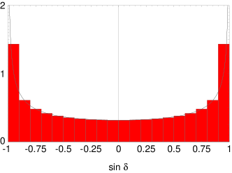
Since the angles $\eta$, $\phi_{1,2}$ are unphysical while the angles $\chi_{1,2}$ are Majorana phases relevant only to lepton-number violating processes, we focus only on $\sin^{2}2\theta_{ij}$ as well as the CP-violating parameter $\sin\delta$ which is the dependence on $\delta$ in neutrino oscillations. It turns out that the distributions in $\sin^{2}2\theta_{ij}$ are all the same. In Fig. 2, we show distributions in $\sin^{2}2\theta_{ij}$ and $\sin\delta$. The solid lines show the differential distributions and the histograms are integrated probabilities with the bin size of $0.1$.

Figure 2: Distributions in (a) $\sin^{2}2\theta_{12}$ or $\sin^{2}2\theta_{13}$ or $\sin^{2}2\theta_{23}$ and (b) $\sin\delta$ for the case of complex mass matrices.

The distributions shown in Ref. [1] used different parameterization of the angles and are consistent with what we show for the case of real matrices except for the following small correction. There, the elements of the mass matrices were scanned from $-1$ to $1$ independently, which forms a hypercube. But such a scan unfortunately breaks the basis-independence as the orientation of the hypercube changes as the basis rotates. This resulted in a small distortion of the distributions, which made them different for Dirac, Majorana, and seesaw cases. We redid the scan with the same programs used in Ref. [1] with a basis-independent boundary ${\rm Tr}M^{\dagger}M\leq 1$, which forms a hypersphere instead, and verified that the distributions obtained from the analytic arguments result from numerical scans.

3.5 Typical Mass Spectrum

The mass spectrum from random mass matrices depends in general on the particular choice of the measure, unlike the distributions in the angles. This is because one can introduce an additional weight factor which depends only on the mass eigenvalues on top of the linear measure as discussed earlier. In this subsection, we use the linear measure throughout, and show what mass spectrum results from this choice. In order to keep basis-independence of the measure, we use the scanning region ${\rm Tr}M^{\dagger}M\leq 1$. This translates to the condition $m_{1}^{2}+m_{2}^{2}+m_{3}^{2}\leq 1$, i.e., to the region inside a three-dimensional sphere.

The first distribution we show is the mass spectrum in the complex Majorana case, with the measure Eq. (17). The distributions in Dirac and real cases are similar and we focus on this case. We take the convention $0<m_{1}<m_{2}<m_{3}$ without a loss of generality. Fig. 3, we show distributions in three mass eigenvalues. We can see that there is a sharp cutoff at $m_{3}=1$ because of the condition $m_{1}^{2}+m_{2}^{2}+m_{3}^{2}\leq 1$. An interesting point is that the other eigenvalues are often much smaller than $O(1)$, almost a half (one) order of magnitude for $m_{2}$ ($m_{1}$). The mass spectrum is somewhat hierarchical. This is rather counter-intuitive as we have only $O(1)$ numbers in the mass matrix. One can qualitatively understand this point as a consequence of two simple facts. The first is that one can regard $(m_{1},m_{2},m_{3})$ as a randomly oriented vector inside the sphere. Consider only the octant where all components are positive. Then it is easy to see that it does not happen very often to have the vector pointing toward the center of the octant where all eigenvalues are $O(1)$. It often fluctuates to be close to one of the planes, where one of the eigenvalues becomes small compared to others. But having two eigenvalues small requires the vector to point close to one of the axes, which is less likely. The second fact is that the measure has the factor $(m_{1}^{2}-m_{2}^{2})(m_{2}^{2}-m_{3}^{2})(m_{3}^{2}-m_{1}^{2})$ which further pulls three eigenvalues apart from each other. As discussed in more detail in the Appendix, this factor reflects the fact that the diagonalization matrix becomes undetermined when two of the eigenvalues become degenerate, and therefore it must be there for any choice of the measure. Unless the unknown weight factor which may be present on top of the linear measure has singularities when some of the eigenvalues coincide, the effect of this factor remains. Therefore, obtaining small hierarchy among three eigenvalues is a rather general consequence of random matrices.

Figure 3: The distributions of mass eigenvalues for the complex Majorana case with the linear measure.

The second distribution we show is the mass spectrum in the complex seesaw case, with the measure Eq. (21). Recall that one needs to diagonalize the seesaw mass matrix Eq. (22) to obtain mass eigenvalues of light (dominantly left-handed) neutrino states. In Fig. 4, we show distributions in three mass eigenvalues. The hierarchy among the eigenvalues is larger than that in the complex Majorana case. First of all, there is no cutoff at $m_{3}=1$ because the seesaw formula involves the inverse of the mass matrix, whose eigenvalue can be larger than 1. The smaller hierarchies in the right-handed Majorana mass matrix and the Dirac mass matrix work together to produce a larger hierarchy in the seesaw mass matrix.

Figure 4: The distributions of mass eigenvalues for the complex seesaw case with the linear measure.

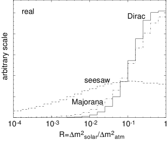
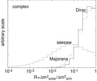
Since the anarchy does not specify the overall scale of the neutrino mass matrix elements, the useful quantity is the ratio of two $\Delta m^{2}$ to compare the consequence of the anarchy and the phenomenology of neutrino oscillation. The Fig. 5 shows the ratio of two $\Delta m^{2}$: $R=(m_{2}^{2}-m_{1}^{2})/(m_{3}^{2}-m_{2}^{2})$ for most of the time ($\sim 90\%$), but when $R>1$, we switch two $\Delta m^{2}$ and define $R=(m_{3}^{2}-m_{2}^{2})/(m_{2}^{2}-m_{1}^{2})$. We will compare this ratio to the observed hierarchy between two $\Delta m^{2}$ relevant to the solar and atmospheric neutrino oscillations. For both real and complex mass matrices, the Dirac and Majorana cases prefer two $\Delta m^{2}$ to be close to each other, while the seesaw cases prefer a hierarchy between two $\Delta m^{2}$ of about a factor of 20. This behavior could be expected from the distribution of mass eigenvalues Figs. 3 and 4.

Figure 5: The distribution of the ratio $R$ of two $\Delta m^{2}$ for real and complex mass matrices.

4 Neutrino Phenomenology

Now we are in the position to compare the consequences of the anarchy to the phenomenology of neutrino oscillation.

4.1 Is The Near-Maximal Mixing Special?

One of the initial reaction to the apparent maximal mixing in the atmospheric data is why the nature prefers to be at the boundary of the physical region: $0\leq\sin^{2}2\theta\leq 1$. This observation led to the wide-spread notion that the neutrino mass matrix must have a very particular structure. We point out in this section that this reaction is based on the use of the incorrect parameter space. As we have seen above, the “correct” parameter to use is $\theta$ for real matrices or $\sin^{2}\theta$ for complex matrices rather than $\sin^{2}2\theta$. Once the correct parameter is used, the current atmospheric data do not seem to require any particular structure.

First we point out that the apparent maximal mixing is not at the boundary of the physical region, but rather at the center of the parameter space. Traditionally, the neutrino oscillation data had been plotted against $\sin^{2}2\theta$, but this covers only a half of the parameter space $0\leq\theta\leq\frac{\pi}{4}$ (the light side). There is another half $\frac{\pi}{4}\leq\theta\leq\frac{\pi}{2}$ (the dark side) which is physically distinct from the light side as we will briefly explain below.

Neutrino oscillations occur if neutrino mass eigenstates are different from neutrino weak eigenstates. Assuming that only two neutrino states mix, the relation between mass eigenstates ($\nu_{1}$ and $\nu_{2}$) and flavor eigenstates (for example $\nu_{e}$ and $\nu_{\mu}$) is simply given by

$$|\nu_{1}\rangle = \cos\theta|\nu_{e}\rangle-\sin\theta|\nu_{\mu}\rangle,$$

$$|\nu_{2}\rangle = \sin\theta|\nu_{e}\rangle+\cos\theta|\nu_{\mu}\rangle,$$ (25)

where $\theta$ is the vacuum mixing angle. The mass-squared difference is defined as $\Delta m^{2}\equiv m_{2}^{2}-m_{1}^{2}$. We are interested in the range of parameters that encompasses all physically different situations. First, observe that Eq. (4.1) is invariant under $\theta\rightarrow\theta+\pi$, $|\nu_{e}\rangle\rightarrow-|\nu_{e}\rangle$, $|\nu_{\mu}\rangle\rightarrow-|\nu_{\mu}\rangle$, and hence the ranges $[-\frac{\pi}{2},\frac{\pi}{2}]$ and $[\frac{\pi}{2},\frac{3\pi}{2}]$ are physically equivalent. Next, note that it is also invariant under $\theta\rightarrow-\theta$, $|\nu_{\mu}\rangle\rightarrow-|\nu_{\mu}\rangle$, $|\nu_{2}\rangle\rightarrow-|\nu_{2}\rangle$, hence it is sufficient to only consider $\theta\in[0,\frac{\pi}{2}]$. Finally, it can also be made invariant under $\theta\rightarrow\frac{\pi}{2}-\theta$, $|\nu_{\mu}\rangle\rightarrow-|\nu_{\mu}\rangle$ by relabeling the mass eigenstates $|\nu_{1}\rangle\leftrightarrow|\nu_{2}\rangle$, i.e. $\Delta m^{2}\rightarrow-\Delta m^{2}$. Thus, we can take ($\Delta m^{2}>0$) without a loss of generality. All physically different situations are obtained by allowing $0\leq\theta\leq\frac{\pi}{2}$. This very simple yet often forgotten point, that maximal mixing $\theta=\pi/4$ is not at the boundary of the parameter space but rather at the center of the continuum, has important implications on the perception. This has already been emphasized in the context of model building [3].

For the case of oscillations in the vacuum, the survival probability is given by

$$P(\nu_{e}\rightarrow\nu_{e})=1-\sin^{2}2\theta\sin^{2}\left(1.27\frac{\Delta m^{2}}{E}L\right).$$ (26)

Here, $\Delta m^{2}$ is given in eV${}^{2}/c^{4}$, $E$ in GeV, and $L$ in km. In this case the oscillation phenomenon can be parameterized by $\Delta m^{2}$ and $\sin^{2}2\theta$, since $\theta$ and $\frac{\pi}{2}-\theta$ yield identical survival probabilities. Therefore we can restrict ourselves to $0\leq\theta\leq\frac{\pi}{4}$, and use the parameter space $(\Delta m^{2},\sin^{2}2\theta)$ without any ambiguity. This is indeed an adequate parameterization for reactor antineutrino oscillation experiments, short-baseline accelerator neutrino oscillation experiments, and $\nu_{\mu}\leftrightarrow\nu_{\tau}$ atmospheric neutrino oscillation experiments.

On the other hand, the effect of matter in neutrino propagation clearly distinguishes the light side from the dark side. One such case is the so-called MSW (Mikheyev–Smirnov–Wolfenstein) effect on the neutrino propagation in the Sun. The survival probability of the electron-neutrino is given by [4]

$$P(\nu_{e}\rightarrow\nu_{e}) = P_{1}\cos^{2}\theta+(1-P_{1})\sin^{2}\theta$$ (27)

$$-\sqrt{P_{c}(1-P_{c})}\cos 2\theta_{M}\sin 2\theta\cos\left(2.54\frac{\Delta m^{2}}{E}L+\delta\right),$$

where $P_{c}$ is the hopping probability, $\theta_{M}$ is the mixing angle at the production point, $P_{1}=P_{c}\sin^{2}\theta_{M}+(1-P_{c})\cos^{2}\theta_{M}$, and $\delta$ is a phase induced by the matter effects, which is not important for our purposes. See Ref. [5, 6] for notation. One can write down an analytic formula for the electron-neutrino survival probability if the electron number density profile in the Sun is approximated by an exponential $n_{e}\propto e^{-r/r_{0}}$:

$$P_{c}=\frac{e^{-\gamma\sin^{2}\theta}-e^{-\gamma}}{1-e^{-\gamma}},$$ (28)

where $\gamma=2\pi r_{0}\Delta m^{2}/2E$. It is easy to check that the survival probability is invariant under the simultaneous change $\Delta m^{2}\rightarrow-\Delta m^{2}$ and $\theta\rightarrow\frac{\pi}{2}-\theta$, but not individually. Therefore the matter effect distinguishes the light and the dark sides.

It cannot be overemphasized that physics is different between the light and the dark side even if the neutrino propagates in the vacuum. It is just that the vacuum oscillation probability comes out the same in both sides. In the case of $\nu_{\mu}$–$\nu_{\tau}$ mixing, for instance, one can ask the question if the mass eigenstate closer to the $\nu_{\mu}$ state is heavier or lighter. If one can literally weigh them, this question has a clear physical meaning. The fact that the vacuum oscillation does not distinguish both sides is simply due to the focus on one particular physical quantity.

4.2 Atmospheric Neutrino Data

Given the fact that the light and the dark sides are physically distinct, it is useful to plot the preferred parameter range from the SuperKamiokande experiment continuously from $0^{\circ}$ to $90^{\circ}$. In Fig. 6, we show plots on $\sin^{2}2\theta$ and $\sin^{2}\theta$ axes. Even though the preferred region appears very close to the maximal angle with the $\sin^{2}2\theta$ plot, it does not on the other plots. In fact, we argued in the previous section that the plot should be shown on the $\sin^{2}\theta$ (rather than $\sin^{2}2\theta$) parameter.

Figure 6: The preferred region from the fit to the atmospheric neutrino data from the SuperKamiokande experiment at 90% and 99% C.L. (a) As it is presented by the collaboration. (b) The dark side is added. (c) Replotted on $\sin^{2}\theta$. The angle $\theta$ is approximately $\theta_{23}$ if $\theta_{13}$ is small enough.

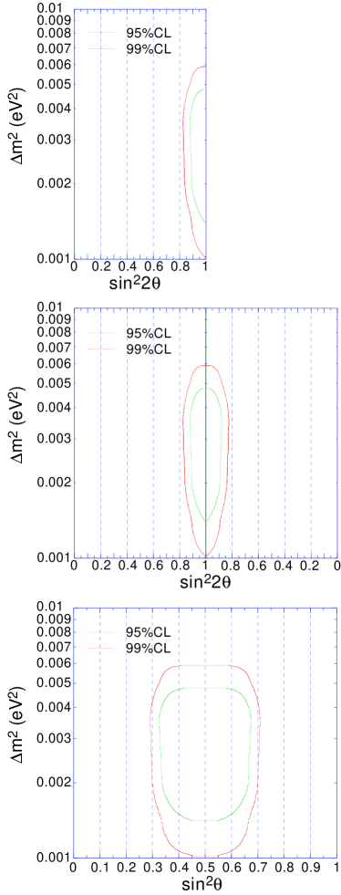
The plots clearly show that the region preferred by the SuperKamiokande atmospheric neutrino data is a somewhat large “blob” at the center of the parameter space, and is not necessarily special. At this point, we can say that a random mass matrix can well produce the apparent “near-maximal” angle. In this sense, we have been fooled by the plots on $\sin^{2}2\theta$ because it shrinks the large angle region.

The atmospheric neutrino data sets the scale for the larger of two $\Delta m^{2}$ to be at 1–6$\times 10^{-3}$ eV².

4.3 Solar Neutrino Data

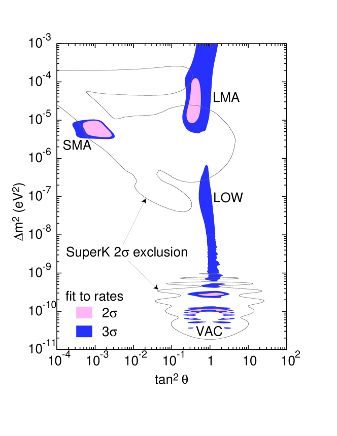
As for the solar neutrino problem, the small hierarchy among $\Delta m^{2}$ in the seesaw case (see Fig. 5) strongly favor the Large Mixing Angle (LMA) MSW solution which requires $\Delta m^{2}=10^{-5}$–$10^{-3}$ eV², especially its upper end (Fig. 7). Recall that $\Delta m^{2}$ for the atmospheric neutrino oscillation is at $10^{-3}$–$10^{-2}$ eV² as discussed in the previous section (Fig. 6). Since we know that $\theta_{13}$ has to be somewhat small (we will come back to this in the next subsection), two-flavor analysis of the solar neutrino oscillation is basically valid even when three flavors are considered. For the LMA solution, the mixing angle is $\sin^{2}2\theta=0.5$–$1$. Recent analysis including the dark side suggest $\tan^{2}\theta=0.15$–$2$ [7]. This is the region where the distribution in $\theta_{12}$ is indeed peaked. Therefore, it is fair to say that the LMA solution is “right on the mark” for the anarchy with no physical distinction among three generations of left-handed lepton doublets.

Figure 7: The preferred regions from the fit to the solar neutrino rates SuperKamiokande, Gallium experiments, and Homestake, taken from Ref. [4]. Overlaid is the 95% CL exclusion from the SuperKamiokande day/night energy spectra [8]. The angle $\theta$ is approximately $\theta_{12}$ if $\theta_{13}$ is small enough.

4.4 Reactor Neutrino Data

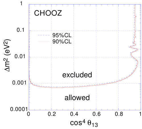
The only quantity where the distribution tends to go against the experimental data is the angle $\theta_{13}$. The lack of $\bar{\nu}_{e}$ disappearance in the reactor neutrino experiments such as CHOOZ and Palo Verde had placed a limit on $|U_{e3}|=\sin\theta_{13}$ (in case $\Delta m^{2}_{12}>\Delta m^{2}_{23}$, it is on $|U_{e1}|$). In Fig. 8, we replot the constraint from the CHOOZ experiment [9] against $\cos^{4}\theta_{13}$ which is the variable that makes the distribution flat according to the $U(3)$ Haar measure. Depending on the precise value of $\Delta m^{2}$ for the atmospheric neutrino oscillation, one obtains $\cos^{4}\theta_{13}>0.7$–$0.95$. The experimentally allowed window is hence 5–30%. We, however, do not see this as a fatal problem for the anarchy. Three out of four physical quantities, $\sin^{2}2\theta_{23}$, $\sin^{2}2\theta_{12}$, and $(\Delta m^{2})_{\odot}/(\Delta m^{2})_{\rm atm}$ worked out right on, and the last one needs a little bit of fluctuation. What this means instead is that $U_{e3}$ may well be just below the current limit.

Figure 8: The limit on $\theta_{13}$ from the CHOOZ reactor anti-neutrino oscillation experiment. It is plotted against $\cos^{4}\theta_{13}$.

5 Hierarchy

In the previous subsections, we have shown that we expect large mixing angles, quite often “maximal,” and only a small hierarchy among mass eigenvalues when there is no fundamental distinction among three generations. The next obvious question then is what generates small angles and large hierarchy for quarks. The charged leptons also have a large hierarchy in their mass eigenvalues.

The most promising approach to this questions is probably an approximate flavor symmetry. The idea is that there is a new symmetry (and hence a new conservation law) which forbids all Yukawa couplings but for the top quark. The symmetry is assumed to be broken by a small parameter, and other Yukawa couplings are generated only at certain powers of the small symmetry breaking parameter. As emphasized in the Introduction, the top Yukawa coupling (and possibly bottom and tau Yukawa couplings if $\tan\beta\sim 60$ in two-doublet Higgs models including the MSSM) is regarded as of natural size $O(1)$, and all other Yukawa couplings are small and hence require explanations. The virtue of the approximate flavor symmetry is that it explains the hierarchical mass eigenvalues as well as the small mixings at the same time.

Then our view of the fermion masses and mixings are simple: there is no distinction among three left-handed lepton doublets $L_{i}$, while there is for right-handed lepton singlets $e_{i}$ as well as quarks. The lack of distinction among $L_{i}$ would appear “anarchical” leading to large mixing angles and small hierarchies in the neutrino sector. However the distinction among three $e_{i}$ as well as quarks due to their different flavor quantum numbers lead to hierarchical masses and small quark mixing angles. This was the simple model presented in [1].

The most simple extension of such model to the whole fermion masses is based on the following $U(1)$ flavor symmetry. The charge assignment is $SU(5)$-like:

$$\begin{array}[]{ccc}\underline{10}_{1}({\bf+2})&\underline{10}_{2}({\bf+1})&\underline{10}_{3}({\bf 0})\\ \underline{5}^{*}_{1}({\bf 0})&\underline{5}^{*}_{2}({\bf 0})&\underline{5}^{*}_{3}({\bf 0})\\ \underline{1}_{1}({\bf 0})&\underline{1}_{2}({\bf 0})&\underline{1}_{3}({\bf 0})\end{array}$$ (29)

where the subscripts are generation indices and the $U(1)$ flavor charges are given in bold face. The $SU(5)$-like multiplets contain $\underline{10}=(Q,u^{c},e^{c})$, $\underline{5}^{*}=(L,d^{c})$, and $\underline{1}=N^{c}$ where $N=\nu_{R}$ is the right-handed neutrino state. The idea here is that the hierarchy in the fermion masses and mixings are solely due to the $\underline{10}$’s. Assuming that the $U(1)$ flavor symmetry is broken by a single parameter $\epsilon({\bf-1})\sim 0.04\sim\lambda^{2}$, the Yukawa matrices read

$$Y_{u}\sim\left(\begin{array}[]{ccc}\epsilon^{4}&\epsilon^{3}&\epsilon^{2}\\ \epsilon^{3}&\epsilon^{2}&\epsilon\\ \epsilon^{2}&\epsilon&1\end{array}\right),\,Y_{d}\sim\left(\begin{array}[]{ccc}\epsilon^{2}&\epsilon^{2}&\epsilon^{2}\\ \epsilon&\epsilon&\epsilon\\ 1&1&1\end{array}\right),\,Y_{l}\sim\left(\begin{array}[]{ccc}\epsilon^{2}&\epsilon&1\\ \epsilon^{2}&\epsilon&1\\ \epsilon^{2}&\epsilon&1\end{array}\right),\,Y_{\nu}\sim\left(\begin{array}[]{ccc}1&1&1\\ 1&1&1\\ 1&1&1\end{array}\right),$$ (30)

where the left-handed (right-handed) fields couple to them from the left (right) of the matrices. There are “random” $O(1)$ coefficients in each of the matrix elements. The property that $Y_{d}\sim Y_{l}^{T}$ is true in many $SU(5)$-like models. Finally, the Majorana mass matrix of right-handed neutrinos is

$$M_{R}\sim M_{0}\left(\begin{array}[]{ccc}1&1&1\\ 1&1&1\\ 1&1&1\end{array}\right),$$ (31)

where $M_{0}\sim 10^{15}$ GeV is the mass scale of lepton-number violation.

Interestingly, these mass matrices had been already discussed in the literature [10], but there has been a perception that the $O(1)$ coefficients as well as texture zeros have to be chosen very carefully. Similar mass matrices had been obtained in the context of composite models [11, 12], extra dimensions [13], and anomalous $U(1)$ [14]. We certainly do not claim that the above mass matrices are new. However, before the analysis in [1], these mass matrices had not been taken seriously as they were not believed to explain the atmospheric and solar neutrino oscillations simultaneously unless careful adjustments and/or more flavor symmetries are imposed in the above-cited papers. Our proposal is that this simple flavor $U(1)$ symmetry is enough to understand the observed pattern of quark, lepton masses, quark mixings and neutrino oscillations based on the simple assumption that the $O(1)$ coefficients would appear pseudo-random from the low-energy point of view.

The above mass matrices would naturally explain (1) the “double” hierarchy in up quarks relative to the hierarchy in down quarks and charged leptons, (2) $V_{cb}\sim O(\epsilon)\sim O(\lambda^{2})$, (3) the similarity between the down quark and charged lepton masses. Some “concerns” with the above mass matrices would be that the following points may be difficult to understand: (a) $m_{s}\sim m_{\mu}/3$, (b) $m_{e}\sim m_{d}/3$, (c) $V_{us}\sim\epsilon^{1/2}$ rather than $\epsilon$. However, in view of the fact that the $O(1)$ coefficients would seem “anarchical” from the low-energy point of view, a factor of $1/3$ is quite likely to appear. And once $m_{s}$ is fluctuated downwards by a factor of $\sim 1/3$, $V_{us}$ would fluctuate upwards to $\sim 3\epsilon$ which is enough to understand the observed pattern of masses and mixings.

What if the $SU(5)$-GUT is true? One can still understand the pseudo-randomness of the $O(1)$ coefficients in the down and lepton masses in the following fashion. Suppose there are many vector-like multiplets at the GUT-scale which do not survive below the GUT-scale simply because of their vector-like nature (“survival hypothesis” [15]). However, they can mix significantly with our quarks and leptons as long as they share the same flavor quantum numbers. The mixing is likely to pick up the $SU(5)$-breaking order parameter, such as the vacuum expectation value of the $SU(5)$-adjoint Higgs boson. Then the resulting low-energy Yukawa couplings would not respect $SU(5)$ invariance and hence would appear random independently between the down quarks and charged leptons. It is simply that the complexity of physics at the GUT-scale leads to a pseudo-random nature of the $O(1)$ coefficients from the low-energy point of view.

Note that we could have assigned non-trivial charges to right-handed neutrino states, and would obtain exactly the same phenomenologies for quarks, charged leptons and neutrino oscillations.

6 Conclusions

We have advocated a new approach to build models of fermion masses and mixings, namely anarchy. The approach relies only on the approximate flavor symmetries, and scan the $O(1)$ coefficients randomly. The randomness in $O(1)$ coupling constants is indeed what one expects in models which are sufficiently complicated or which have a large number of fields mixed with each other.

This approach is particularly useful for neutrinos. Assuming there is no physical distinction among three generations of neutrinos, we have shown that the probability distributions in MNS mixing angles could be predicted independent of the choice of the measure. This is because the mixing angles are distributed to the Haar measure of the Lie groups whose elements diagonalize the mass matrices. The near-maximal mixings, as observed in the atmospheric neutrino data and is required in the LMA solution to the solar neutrino problem, are highly probable. Even though somewhat more dependent on the particular choice of the measure, the distributions in the mass spectrum can also be worked out. A small hierarchy between the $\Delta m^{2}$ for the atmospheric and the solar neutrinos is obtained very easily; the complex seesaw case gives a hierarchy of a factor of 20 as the most probable one. Therefore, these three observables are nicely consistent with the current experimental data. On the other hand, the $U_{e3}$ angle must lie in the 10% tail of the distribution. It is not surprising, however, that three out of four observables are “right on the mark,” while the fourth one is off at the 10% level. In other words, we expect $U_{e3}$ to be just below the current limit from the CHOOZ experiment. This is an ideal situation for the future long-baseline neutrino oscillation experiments. Moreover, CP-violating parameter $\sin\delta$ is preferred to be maximal.

The anarchy can be easily extended to the charged lepton and quark sectors. We presented a simple $SU(5)$-like flavor charge assignment which works well phenomenologically.

Appendix A Measures

A.1 Decomposition of the Measures

The measure over the mass matrix elements can be studied analytically. We consider Majorana and Dirac cases with both real and complex matrix elements. The aim here is to decompose the measure into that over the diagonalization matrix and other over the mass eigenvalues.

First of all, it is important to note that the linear measure over the mass matrix elements is invariant under change of basis. This is because a $N\times N$ real Majorana mass matrix transforms as a symmetric rank-two tensor under the $O(N)$ rotation of the basis $M\rightarrow OMO^{T}$, and hence a linear representation. The naive $N(N+1)/2$-dimensional measure $dM$ is hence invariant under this $O(N)$ rotation. Similarly, a complex Majorana mass matrix transforms as a symmetric rank-two tensor under the $U(N)$ rotation $M\rightarrow UMU^{T}$, a real Dirac mass matrix as $(\underline{N},\underline{N})$ under $O(N)\times O(N)$ as $M\rightarrow O_{L}MO_{R}^{T}$, and a complex Dirac mass matrix as $(\underline{N},\underline{N})$ under $U(N)\times U(N)$ as $M\rightarrow U_{L}MU_{R}^{T}$.

This observation allows us to separate the measure over the mass matrix elements in terms of eigenvalues and group transformations. Starting with the real Majorana case, any mass matrix can be written as

$$M=ODO^{T},$$ (32)

where $O\in SO(N)$ and $D=\mbox{diag}(m_{1},m_{2},\cdots,m_{N})$ is a real diagonal matrix. Because of the invariance of the measure $dM$ under the change of basis $M\rightarrow O_{1}MO_{1}^{T}$, the measure $dM$ should contain the measure over the group $dO$ which is invariant under the left transformation $O\rightarrow O_{1}O$. Since $SO(N)$ is a compact Lie group, a left-invariant measure is also right-invariant. Therefore, $dO$ should be the invariant Haar measure over the group $SO(N)$. Then the measure $dM$ can be written as

$$dM=f(m_{1},\cdots,m_{N})\prod_{i=1}^{N}dm_{i}dO.$$ (33)

Here the yet-undetermined function $f$ is symmetric under the interchange of eigenvalues. However, when two of the eigenvalues coincide, an $SO(2)$ subgroup of the $SO(N)$ becomes ill-defined and we expect zeros in the function $f$. Therefore, $f\propto\prod_{i<j}^{N}(m_{i}-m_{j})$. This factor already saturates the dimension of the measure, and hence

$$dM=\prod_{i<j}(m_{i}-m_{j})\prod_{i=1}^{N}dm_{i}dO$$ (34)

up to a constant normalization factor. As we will see below, this simple expression allows us to study the distributions in the mixing angles and eigenvalues very easily.

A similar consideration for the real Dirac case leads to the following measure:

$$dM=\prod_{i<j}(m_{i}^{2}-m_{j}^{2})\prod_{i=1}^{N}dm_{i}dO_{L}dO_{R}.$$ (35)

Here, the mass matrix is parameterized as $M=O_{L}DO_{R}^{T}$, and $dO_{L,R}$ are Haar measures of both $O(N)$ factors. If we restrict $O_{L,R}$ matrices to $SO(N)$, we must allow both positive and negative eigenvalues. However, in the vicinity of $O_{L,R}=1$, one can change the basis by an $O(N)$ rotation $\mbox{diag}(1,\cdots,1,-1,1,\cdots,1)$ to flip sign of one of the eigenvalues, and hence $m_{i}=-m_{j}$ should give a singularity as well as $m_{i}=m_{j}$. Therefore, the prefactor should be $\prod_{i<j}(m_{i}^{2}-m_{j}^{2})$ which saturates the dimension and hence is unique up to a normalization constant.

The complex Majorana case is given by

$$dM=\prod_{i<j}(m_{i}^{2}-m_{j}^{2})\prod_{i=1}^{N}m_{i}dm_{i}dU.$$ (36)

The mass matrix is parameterized as $M=UDU^{T}$ where $U\in U(N)$. The prefactor can be determined by the same argument as in the real Dirac case, because the sign of an eigenvalue can be flipped by an $U(N)$ rotation ${\rm diag}(1,\cdots,1,i,1,\cdots,1)$. However this does not saturate the dimension of the measure, leaving additional $N$ powers of the eigenvalues. Only such an additional factor which is symmetric under the interchange and also invariant under the change of the sign of an eigenvalue up to an overall sign is the product of all eigenvalues, $\prod=i^{N}m_{i}$. Therefore the above parameterization is unique.

Finally the complex Dirac case gives

$$dM=\prod_{i<j}(m_{i}^{2}-m_{j}^{2})^{2}\prod_{i=1}^{N}m_{i}dm_{i}\frac{dU_{L}dU_{R}}{\prod_{i}^{N}d\phi_{i}}.$$ (37)

The parameterization is $M=U_{L}DU_{R}^{\dagger}$. The prefactor is based on the same argument as the real Dirac and complex Majorana cases, and the reason why $(m_{i}^{2}-m_{j}^{2})$ factor is squared is because $U(2)$ subgroups of $U_{L}$ and $U_{R}$ rotations are not independent when $m_{i}=m_{j}$. We verified this for $N=2$, and this conjecture appears to be the unique generalization to arbitrary $N$. The group measure is modded out by the following transformation $U_{L,R}\rightarrow TU_{L,R}$, where $T=\mbox{diag}(e^{i\phi_{1}},e^{i\phi_{2}},\cdots,e^{i\phi_{N}})$, because this simultaneous change of $U_{L}$ and $U_{R}$ does not change the mass matrix $M$.

Note that we do not quite know on what measure we should regard the mass matrix elements to be “random.” The measure we discussed above, namely the linear measure over the mass matrix elements may not necessarily be the correct measure. However, the requirement of the basis independence implies that the invariant Haar measure is certainly a part of it. The only possible modification of the linear measure discussed above is a weight function which depends on the symmetric polynomials of the eigenvalues. Therefore, the distributions on the mass eigenvalues can change from the linear measure to the “correct” one, but the distributions on the mixing angles cannot.

A.2 Haar Measures

The invariant Haar measures of $SO(3)$ and $U(3)$ groups relevant to our study can be obtained once their parameterization is fixed.

First define the (right) Maurer–Cartan forms on the group manifold $G$

$$\omega^{a}=-i{\rm Tr}T^{a}U^{-1}dU$$ (38)

where $U\in G$. Here, $T^{a}$ are hermitian generators. It is easy to check that these forms are trivially invariant under the left-translation of the group $U\rightarrow U_{0}U$. Under the right-translations $U\rightarrow UU_{0}$, however, they transform among each other:

$$\omega^{a}\rightarrow O_{0}^{ab}\omega^{b},$$ (39)

where

$$U_{0}T^{a}U_{0}^{-1}=O^{ab}T^{b}.$$ (40)

Note that $O_{0}$ is an orthogonal matrix, which is easily checked by doing a successive left-translation by $U_{0}^{-1}$. Because the Maurer–Cartan forms transform homogeneously by an orthogonal matrix, the following combination

$$dU=\epsilon_{a_{1}a_{2}\cdots a_{N}}\omega^{a_{1}}\wedge\omega^{a_{2}}\wedge\cdots\wedge\omega^{a_{N}}$$ (41)

is invariant under the right-translations. Here, $\epsilon_{a_{1}a_{2}\cdots a_{N}}$ is the totally anti-symmetric tensor. This measure is invariant because of the orthogonal nature of the transformation, and $N={\rm dim}G$.

For $SO(3)$, take the conventional parameterization

$$O = \left(\begin{array}[]{ccc}1&0&0\\ 0&c_{23}&s_{23}\\ 0&-s_{23}&c_{23}\end{array}\right)\left(\begin{array}[]{ccc}c_{13}&0&s_{13}\\ 0&1&0\\ -s_{13}&0&c_{13}\end{array}\right)\left(\begin{array}[]{ccc}c_{12}&s_{12}&0\\ -s_{12}&c_{12}&0\\ 0&0&1\end{array}\right)$$ (51)

$$= \left(\begin{array}[]{ccc}c_{12}c_{13}&s_{12}c_{13}&s_{13}\\ -s_{12}c_{23}-c_{12}s_{23}s_{13}&c_{12}c_{23}-s_{12}s_{23}s_{13}&s_{23}c_{13}\\ s_{12}s_{23}-c_{12}c_{23}s_{13}&-c_{12}s_{23}-s_{12}c_{23}s_{13}&c_{23}c_{13}\end{array}\right),$$ (55)

where $c_{12}=\cos\theta_{12}$ etc. Then the Haar measure is given by

$$dO=\cos\theta_{13}d\theta_{12}d\theta_{13}d\theta_{23}$$ (56)

up to an overall normalization factor. Note that the measure is flat in $\theta_{12}$ and $\theta_{23}$ similarly to the two-generation Majorana case discussed earlier. Therefore these distributions are peaked in $\sin^{2}2\theta_{12}$ and $\sin^{2}2\theta_{23}$ both at $0$ and $1$. The measure is different for $\theta_{13}$ being in the middle among three rotations. The reason why the measure is degenerate when $\theta_{13}\rightarrow\pi/2$ is that $\theta_{12}$ and $\theta_{23}$ are not independent at this point.

For $U(3)$, take a similar parameterization

$$U=e^{i\eta}e^{i\phi_{1}\lambda_{3}+i\phi_{2}\lambda_{8}}\left(\begin{array}[]{ccc}1&0&0\\ 0&c_{23}&s_{23}\\ 0&-s_{23}&c_{23}\end{array}\right)\left(\begin{array}[]{ccc}c_{13}&0&s_{13}e^{-i\delta}\\ 0&1&0\\ -s_{13}e^{i\delta}&0&c_{13}\end{array}\right)\left(\begin{array}[]{ccc}c_{12}&s_{12}&0\\ -s_{12}&c_{12}&0\\ 0&0&1\end{array}\right)e^{i\chi_{1}\lambda_{3}+i\chi_{2}\lambda_{8}},$$ (57)

where $\lambda_{3}={\rm diag}(1,-1,0)$ and $\lambda_{8}={\rm diag}(1,1,-2)/\sqrt{3}$ are Gell-Mann matrices. This parameterization is designed to make the angles $\eta$, $\phi_{1,2}$, $\chi_{1,2}$ unphysical except for the Majorana phases in possible lepton-number violating processes. Then the Haar measure is given by

$$dU=ds_{12}^{2}dc_{13}^{4}ds_{23}^{2}d\delta d\eta d\phi_{1}d\phi_{2}d\chi_{1}d\chi_{2}$$ (58)

up to an overall normalization factor. For the Dirac mass matrices, we need to mod out linear combinations of $\eta$, $\chi_{1}$, $\chi_{2}$ from $U_{L}$ and $U_{R}$, but this does not affect the measure for physical angles, $\theta_{12}$, $\theta_{13}$, $\theta_{23}$, $\delta$.

References

- [1] L. Hall, H. Murayama and N. Weiner, Phys. Rev. Lett. 84, 2572 (2000) [hep-ph/9911341].
- [2] Mirriam-Webster’s Collegiate Dictionary, online at http://www.m-w.com/. See also http://www.encyclopedia.com/articles/00476.html.
- [3] Y. Nir, JHEP 0006, 039 (2000) [hep-ph/0002168].
- [4] A. de Gouvêa, A. Friedland and H. Murayama, hep-ph/0002064. To appear in Phys. Lett. B.
- [5] A. de Gouvêa, A. Friedland and H. Murayama, Phys. Rev. D60, 093011 (1999) [hep-ph/9904399].
- [6] A. de Gouvêa, A. Friedland and H. Murayama, hep-ph/9910286.
- [7] C. Gonzalez-Garcia, parallel session talk presented at XXXth International Conference on High Energy Physics, Osaka, Japan, July 27–August 2, 2000, http://ichep2000.hep.sci.osaka-u.ac.jp/scan/0728/pa08/gonzalez_garcia/index.html
- [8] Y. Suzuki, talk presented at 19th International Conference On Neutrino Physics And Astrophysics - Neutrino 2000, Sudbury, Ontario, Canada, 16-21 Jun 2000, http://nu2000.sno.laurentian.ca/Y.Suzuki/index.html. HM thanks Dr. Yusuke Koshio for making the PostScript file available to him.
- [9] M. Apollonio et al., Phys. Lett. B466, 415 (1999) [hep-ex/9907037].
- [10] K. S. Babu and S. M. Barr, Phys. Lett. B381, 202 (1996) [hep-ph/9511446]; S. M. Barr, Phys. Rev. D55, 1659 (1997) [hep-ph/9607419].
- [11] M. Strassler, talk presented at International Workshop On Perspectives Of Strong Coupling Gauge Theories (SCGT 96), Nov 13–16, 1996, Nagoya, Japan.
- [12] N. Haba, Phys. Rev. D59, 035011 (1999) [hep-ph/9807552].
- [13] K. Yoshioka, Mod. Phys. Lett. A15, 29 (2000) [hep-ph/9904433].
- [14] J. Hisano, K. Kurosawa and Y. Nomura, Nucl. Phys. B584, 3 (2000) [hep-ph/0002286].
-
[15]
H. Georgi,
Nucl. Phys. B156, 126 (1979);
S. L. Glashow, “The Future Of Elementary Particle Physics,” In *Cargese 1979, Proceedings, Quarks and Leptons*, 687-713 and Harvard Univ.Cambridge - HUTP-79-A059 (79,REC.DEC.) 40p.