The Similarity Renormalization Group

Sérgio Szpigel and Robert J. Perry

Department of Physics
The Ohio State University, Columbus, OH 43210
Abstract

Quantum field theories require a cutoff to regulate divergences that result from local interactions, and yet physical results can not depend on the value of this cutoff. The renormalization group employs a transformation that changes the cutoff to isolate hamiltonians that produce cutoff-independent eigenvalues. The similarity renormalization group is based on similarity transformations that regulate off-diagonal matrix elements, forcing the hamiltonian towards a band-diagonal form as the cutoff is lowered. This avoids pathologies that plagued tradition transformations acting on hamiltonians, making it possible to produce a well-behaved perturbative approximation of renormalized hamiltonians in asymptotically free theories. We employ a simple two-dimensional delta function example to illustrate this new renormalization technique.


1 Introduction

Early attempts to combine quantum mechanics and special relativity led to the consideration of local interactions, which are consistent with causality and avoid signals that propagate faster than light. Local interactions lead to divergences in perturbation theory, whose discovery caused some of the best theorists in the world to question the foundations of quantum mechanics. Eventual successes at fitting precise atomic experimental data led to the universal acceptance of renormalization recipes that were acknowledged to make little sense [1]. Initially the perturbative renormalization of QED required theorists to match perturbative expansions in powers of a bare and physical electronic charge [2], but the bare charge clearly diverges logarithmically in QED and the success of an expansion in powers of such a coupling was mysterious at best [3].

The first steps towards making sense of renormalization theory were taken in the 1950’s with the invention of the perturbative renormalization group  [4, 5, 6, 7, 8], although serious investigators found the theory was still plagued by non-convergent sums because QED is not asymptotically free. The development of Wilson’s renormalization group formalism [9, 10] and the discovery of asymptotic freedom [11] allowed physicists to produce a logically reasonable picture of renormalization in which perturbative expansions at any high energy scale can be matched with one another, with no necessity to deal with intermediate expansions in powers of a large parameter.

In this pedagogical article we take advantage of the fact that the divergences in field theory result entirely from local interactions. To understand the most important aspects of renormalization theory requires only a background in nonrelativistic quantum mechanics, because as has been long known the divergences of field theory are directly encountered when one tries to impose locality on the Schrödinger equation. In this case the interactions we consider that are local at all scales are delta functions and derivatives of delta functions. These divergences can be regulated by the introduction of a cutoff, and the artificial effects of this cutoff must be removed by renormalization. The simplicity of the one-body Schrödinger equation makes it possible to renormalize the theory exactly, disentangling the effects of locality from the complicated many-body effects and symmetry constraints encountered in realistic field theories. There is a large literature on the subject [12]-[29], primarily pedagogical.

The similarity renormalization group (SRG) is a very recent development invented by Stan Głazek and Ken Wilson [30, 31], and independently by Franz Wegner [32]. We do not review the applications of this method, which are growing in number.

In the SRG, as in Wilson’s original renormalization group formalism [33, 34], transformations that explicitly run the cutoff are developed. These transformations are the group elements that give the renormalization group its name.

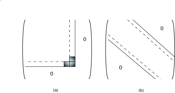
In his earliest work  [33, 34] Wilson exploited a transformation originally invented by Claude Bloch [35]. It uses a cutoff on the states themselves, and as the cutoff is lowered, states are removed from the Hilbert space. If the hamiltonian is viewed as a matrix, these cutoffs can be seen as limiting the size of this matrix and the transformation reduces this size, as illustrated in Fig. 1a. Wilson introduced a rescaling operation to allow transformed hamiltonians to be compared with initial hamiltonians, despite the fact that they act on different spaces; however, the Bloch transformation is ill-defined and even in perturbation theory it leads to artificial divergences. These divergences come from the small energy differences between states retained and states removed by the transformation, and they appear in the form of small energy denominators in the perturbative expansion of the transformed hamiltonian. These small energy denominator problems led Wilson to abandon the hamiltonian formulation of field theory in favor of path integral formulations, but the virtues of the hamiltonian formulation over the path integral formulation for many problems remains.
Refer to caption

Figure 1: Two ways to run a cutoff on free energy. In (a) a cutoff on the magnitude of the energy is lowered from the solid to the dashed lines, with problems resulting from the removed shaded region. In (b) a cutoff on how far off diagonal matrix elements appear is lowered from the dashed to the solid lines.

The breakthrough provided by the SRG is that the transformations are typically unitary, making them well-defined, and they run a cutoff on energy differences rather than on individual states, as illustrated in Fig. 1b. Again viewing the hamiltonian as a large matrix, these cutoffs limit the off-diagonal matrix elements and as they are reduced the hamiltonian is forced towards diagonal form. The perturbative expansion for transformed hamiltonians contains no small energy denominators, so the expansion breaks down only when interactions become sufficiently strong, in which case perturbation theory should fail in any case.

Although the SRG has not yet been applied to a wide range of problems, it may be an important new tool both for attacking field theories and non-relativistic many-body problems.

When the SRG is used with coupling coherence  [36, 37], which we explain below, it allows us to construct effective theories with the same number of free parameters as the underlying ‘fundamental’ theory. For the delta-function example there is one fundamental parameter, the strength of the regulated delta-function as the cutoff is removed. In the SRG with coupling coherence, there is only one fundamental coupling and all new couplings are perturbative functions of the fundamental coupling that are given by coupling coherence. It is the renormalization group flow of the added couplings, and a boundary condition that they vanish when the fundamental coupling is taken to zero, that fixes their dependence on the fundamental coupling.

The examples we use in this article do not illustrate non-Gaussian fixed points, so their scaling properties are driven by naive dimensional analysis. However, we will see that even in these cases scaling behavior of effective hamiltonians derived using a perturbative similarity renormalization group can be very complicated. We will see that in the perturbative SRG there are errors arising from the approximate treatment of the fundamental running coupling and the approximate treatment of the relation between this coupling and the new couplings of irrelevant operators.

In a realistic calculation the marginal coupling, which corresponds to the strength of the regulated delta function, would be fit to data. In order to clearly illustrate the logarithmic errors that result from using the perturbative SRG equations, we approximate this marginal coupling in this article rather than renormalizing it nonperturbatively by fitting data. The strengths of the irrelevant operators, which correspond to derivatives of the regulated delta function, are approximated using expansions in powers of the approximate running coupling that are fixed by coupling coherence. The approximate running coupling differs from the exact running coupling by inverse powers of logarithms of the cutoff, and the error analysis for the binding energy displays the resultant inverse logarithmic errors in addition to power-law errors seen in all approximate renormalization group calculations. In addition there are errors in the strengths of the irrelevant operators resulting from using a truncated expansion in powers of the running coupling and an approximate running coupling, both of which introduce inverse logarithmic errors in addition to the power-law errors normally seen.

The utility of the renormalization group rests on our ability to accurately determine and control the magnitude of errors resulting from the artificial cutoff. For perturbative calculations this issue is not critical, but in all field theories (and in our example) a scale is reached where the coupling becomes large and a non-perturbative calculation must be done. The renormalization group allows us to eliminate as much perturbative physics as possible (i.e., lower the cutoff as far as possible in an asymptotically free theory), so that the essential degrees of freedom that couple non-perturbatively can be isolated.

2 Similarity Renormalization Group

In this section we review the general formulation of the SRG developed by Głazek and Wilson  [30, 31] and a specific transformation developed by Wegner  [32]. The reader may wish to skip the general formulation on a first reading.

2.1 Głazek-Wilson Formulation

Consider a system described by a hamiltonian written in the form

H=h+V,𝐻𝑉H=h+V\;, (1)

where hh is the free hamiltonian and V𝑉V is an interaction.

In general, the hamiltonian can couple states of all energy scales and such couplings can be a source of ultraviolet divergences. The goal of the SRG is to obtain an effective hamiltonian in which the couplings between high and low-energy states are removed, while avoiding any problems from small energy denominators in effective interactions. The procedure is implemented by a unitary transformation that generates effective interactions that reproduce the effects of the eliminated couplings. The effective hamiltonian cannot produce ultraviolet divergences at any order in perturbation theory as long as its matrix elements are finite.

In our discussion we will use the basis of eigenstates of the free hamiltonian,

h|i>=ϵi|i>.ket𝑖subscriptitalic-ϵ𝑖ket𝑖h|i>=\epsilon_{i}|i>\;. (2)

We start by defining a bare hamiltonian, HΛsubscript𝐻ΛH_{\Lambda}, regulated by a very large cutoff ΛΛ\Lambda (here with dimensions of energy) on the change in free energy at the interaction vertices,

HΛsubscript𝐻Λ\displaystyle H_{\Lambda} \displaystyle\equiv h+VΛ,subscript𝑉Λ\displaystyle h+V_{\Lambda}\;, (3)
VΛsubscript𝑉Λ\displaystyle V_{\Lambda} \displaystyle\equiv fΛV¯Λ,subscript𝑓Λsubscript¯𝑉Λ\displaystyle f_{\Lambda}{\overline{V}}_{\Lambda}\;, (4)
V¯Λsubscript¯𝑉Λ\displaystyle{\overline{V}}_{\Lambda} \displaystyle\equiv v+HΛct,𝑣superscriptsubscript𝐻Λ𝑐𝑡\displaystyle v+H_{\Lambda}^{ct}\;, (5)

where fΛsubscript𝑓Λf_{\Lambda} is a “similarity function”, V¯Λsubscript¯𝑉Λ{\overline{V}}_{\Lambda} is defined as the reduced interaction and HΛctsuperscriptsubscript𝐻Λ𝑐𝑡H_{\Lambda}^{ct} are counterterms that must be determined through the process of renormalization in order to remove ΛΛ\Lambda dependence in physical quantities.

The similarity function fΛsubscript𝑓Λf_{\Lambda} regulates the hamiltonian by suppressing matrix elements between free states with significantly large energy difference and acts in the following way:

<i|fΛHΛ|j>quantum-operator-product𝑖subscript𝑓Λsubscript𝐻Λ𝑗\displaystyle<i|f_{{}_{\Lambda}}H_{{}_{\Lambda}}|j> \displaystyle\equiv ϵiδij+fΛ(ϵiϵj)<i|V¯Λ|j>subscriptitalic-ϵ𝑖subscript𝛿𝑖𝑗subscript𝑓Λsubscriptitalic-ϵ𝑖subscriptitalic-ϵ𝑗quantum-operator-product𝑖subscript¯𝑉Λ𝑗\displaystyle\epsilon_{i}\;\delta_{ij}+f_{{}_{\Lambda}}(\epsilon_{i}-\epsilon_{j})<i|{\overline{V}}_{{}_{\Lambda}}|j> (6)
\displaystyle\equiv ϵiδij+fΛijV¯Λij.subscriptitalic-ϵ𝑖subscript𝛿𝑖𝑗subscript𝑓Λ𝑖𝑗subscript¯𝑉Λ𝑖𝑗\displaystyle\epsilon_{i}\;\delta_{ij}+f_{{}_{\Lambda ij}}{\overline{V}}_{{}_{\Lambda ij}}.

Typically, the similarity function is chosen to be a smooth function satisfying

(i)fΛ(ϵiϵj)1,when|ϵiϵj|<<Λ,formulae-sequence𝑖subscript𝑓Λsubscriptitalic-ϵ𝑖subscriptitalic-ϵ𝑗1much-less-thanwhensubscriptitalic-ϵ𝑖subscriptitalic-ϵ𝑗Λ\displaystyle(i)f_{{}_{\Lambda}}(\epsilon_{i}-\epsilon_{j})\rightarrow 1,\;{\rm when}\;|\epsilon_{i}-\epsilon_{j}|<<\Lambda\;,
(ii)fΛ(ϵiϵj)0,when|ϵiϵj|>>Λ.formulae-sequence𝑖𝑖subscript𝑓Λsubscriptitalic-ϵ𝑖subscriptitalic-ϵ𝑗0much-greater-thanwhensubscriptitalic-ϵ𝑖subscriptitalic-ϵ𝑗Λ\displaystyle(ii)f_{{}_{\Lambda}}(\epsilon_{i}-\epsilon_{j})\rightarrow 0,\;{\rm when}\;|\epsilon_{i}-\epsilon_{j}|>>\Lambda\;. (7)

In several papers the similarity function has been chosen to be a step function. Although useful for doing analytic calculations, such a choice can lead to pathologies.

The similarity transformation is defined to act on the bare regulated Hamiltonian, HΛsubscript𝐻ΛH_{\Lambda}, lowering the cutoff down to a scale λ𝜆\lambda:

Hλsubscript𝐻𝜆\displaystyle H_{\lambda} \displaystyle\equiv U(λ,Λ)HΛU(λ,Λ).𝑈𝜆Λsubscript𝐻Λsuperscript𝑈𝜆Λ\displaystyle U(\lambda,\Lambda)\;H_{\Lambda}\;U^{\dagger}(\lambda,\Lambda)\;. (8)

The renormalized Hamiltonian can be written in the general form

Hλsubscript𝐻𝜆\displaystyle H_{\lambda} \displaystyle\equiv h+Vλ,subscript𝑉𝜆\displaystyle h+V_{\lambda}\;, (9)
Vλsubscript𝑉𝜆\displaystyle V_{\lambda} \displaystyle\equiv fλV¯λ.subscript𝑓𝜆subscript¯𝑉𝜆\displaystyle f_{\lambda}\;{\overline{V}}_{\lambda}\;. (10)

The transformation is unitary, so HΛsubscript𝐻ΛH_{\Lambda} and Hλsubscript𝐻𝜆H_{\lambda} produce the same spectra for observables. Also, if an exact transformation is implemented, the physical predictions using the renormalized Hamiltonian must be independent of the cutoff λ𝜆\lambda and HΛctsuperscriptsubscript𝐻Λ𝑐𝑡H_{\Lambda}^{ct} is chosen so that they also become independent of ΛΛ\Lambda as ΛΛ\Lambda\rightarrow\infty.

The unitarity condition is given by:

U(λ,Λ)U(λ,Λ)𝑈𝜆Λsuperscript𝑈𝜆Λ\displaystyle U(\lambda,\Lambda)\;U^{\dagger}(\lambda,\Lambda) \displaystyle\equiv U(λ,Λ)U(λ,Λ)1.superscript𝑈𝜆Λ𝑈𝜆Λ1\displaystyle U^{\dagger}(\lambda,\Lambda)\;U(\lambda,\Lambda)\equiv 1\;. (11)

The similarity transformation U𝑈U can be defined in terms of an anti-hermitian operator Tλsubscript𝑇𝜆T_{\lambda} (Tλ=Tλsuperscriptsubscript𝑇𝜆subscript𝑇𝜆T_{\lambda}^{\dagger}=-T_{\lambda}) which generates infinitesimal changes of the cutoff energy scale,

U(λ,Λ)𝑈𝜆Λ\displaystyle U(\lambda,\Lambda) \displaystyle\equiv 𝒯exp(λΛTλ𝑑λ),𝒯superscriptsubscript𝜆Λsubscript𝑇superscript𝜆differential-dsuperscript𝜆\displaystyle{\cal T}\exp\left(\int_{\lambda}^{\Lambda}T_{\lambda^{\prime}}\;d\lambda^{\prime}\right)\;, (12)

where 𝒯𝒯{\cal T} orders operators from left to right in order of increasing energy scale λsuperscript𝜆\lambda^{\prime}. Using

Tλ=U(λ,Λ)dU(λ,Λ)dλ=dU(λ,Λ)dλU(λ,Λ),subscript𝑇𝜆𝑈𝜆Λ𝑑superscript𝑈𝜆Λ𝑑𝜆𝑑𝑈𝜆Λ𝑑𝜆superscript𝑈𝜆ΛT_{\lambda}=U(\lambda,\Lambda)\;\frac{dU^{\dagger}(\lambda,\Lambda)}{d\lambda}=-\frac{dU(\lambda,\Lambda)}{d\lambda}\;U^{\dagger}(\lambda,\Lambda)\;, (13)

and the unitarity condition Eq. (11), we can write Eq. (8) in a differential form,

dHλdλ𝑑subscript𝐻𝜆𝑑𝜆\displaystyle\frac{dH_{\lambda}}{d\lambda} =\displaystyle= [Hλ,Tλ].subscript𝐻𝜆subscript𝑇𝜆\displaystyle\left[H_{\lambda},T_{\lambda}\right]\;. (14)

This is a first-order differential equation, which is solved with the boundary condition Hλ|λΛHΛevaluated-atsubscript𝐻𝜆𝜆Λsubscript𝐻ΛH_{\lambda}|_{{}_{\lambda\rightarrow\Lambda}}\equiv H_{\Lambda}. The bare Hamiltonian is typically given by the canonical Hamiltonian plus counterterms that must be uniquely fixed to complete the renormalization.

The operator Tλsubscript𝑇𝜆T_{\lambda} is defined by specifying how V¯λsubscript¯𝑉𝜆{\overline{V}}_{\lambda} and hh depend on the cutoff scale λ𝜆\lambda. For simplicity in this article, we demand that hh is independent of λ𝜆\lambda, although this may not lead to an increasingly diagonal effective hamiltonian in all cases. We also demand that no small energy denominators can appear in the hamiltonian. These constraints are implemented by the conditions

dhdλ𝑑𝑑𝜆\displaystyle\frac{dh}{d\lambda} \displaystyle\equiv 0,0\displaystyle 0\;, (15)
dV¯λdλ𝑑subscript¯𝑉𝜆𝑑𝜆\displaystyle\frac{d{\overline{V}}_{\lambda}}{d\lambda} \displaystyle\equiv [Vλ,Tλ].subscript𝑉𝜆subscript𝑇𝜆\displaystyle[V_{\lambda},T_{\lambda}]\;. (16)

To obtain the renormalized Hamiltonian perturbatively, expand

V¯λ=V¯λ(1)+V¯λ(2)+,subscript¯𝑉𝜆superscriptsubscript¯𝑉𝜆1superscriptsubscript¯𝑉𝜆2\displaystyle{\overline{V}}_{\lambda}={\overline{V}}_{\lambda}^{{}^{(1)}}+{\overline{V}}_{\lambda}^{{}^{(2)}}+\cdots~{}, (17)
Tλ=Tλ(1)+Tλ(2)+,subscript𝑇𝜆superscriptsubscript𝑇𝜆1superscriptsubscript𝑇𝜆2\displaystyle T_{\lambda}=T_{\lambda}^{{}^{(1)}}+T_{\lambda}^{{}^{(2)}}+\cdots~{}, (18)
HΛct=HΛ(2),ct+HΛ(3),ct+,superscriptsubscript𝐻Λ𝑐𝑡superscriptsubscript𝐻Λ2𝑐𝑡superscriptsubscript𝐻Λ3𝑐𝑡\displaystyle H_{{}_{\Lambda}}^{{}^{ct}}=H_{{}_{\Lambda}}^{{}^{(2),ct}}+H_{{}_{\Lambda}}^{{}^{(3),ct}}+\cdots\;, (19)

where the superscripts denote the order in the original interaction, V𝑉V. A general form of these effective interactions is

V¯λ(i)superscriptsubscript¯𝑉𝜆𝑖\displaystyle{\overline{V}}_{\lambda}^{{}^{(i)}} =\displaystyle= j,k=1δ(j+k,i)λΛ𝑑λ[Vλ(j),Tλ(k)]+HΛ(i),ct,superscriptsubscript𝑗𝑘1subscript𝛿𝑗𝑘𝑖superscriptsubscript𝜆Λdifferential-dsuperscript𝜆superscriptsubscript𝑉superscript𝜆𝑗superscriptsubscript𝑇superscript𝜆𝑘superscriptsubscript𝐻Λ𝑖𝑐𝑡\displaystyle-\sum_{j,k=1}^{\infty}\delta_{(j+k,i)}\int_{\lambda}^{\Lambda}d\lambda^{\prime}\;[V_{\lambda^{\prime}}^{{}^{(j)}},T_{\lambda^{\prime}}^{{}^{(k)}}]+H_{{}_{\Lambda}}^{{}^{(i),ct}}\;, (20)

for i=2,3,𝑖23i=2,3,\cdots, with V¯λ(1)=vsuperscriptsubscript¯𝑉𝜆1𝑣{\overline{V}}_{\lambda}^{{}^{(1)}}=v. For instance, the explicit form of the second-order effective interaction V¯λ(2)superscriptsubscript¯𝑉𝜆2{\overline{V}}_{\lambda}^{{}^{(2)}} is

V¯λij(2)=kVikVkj(gikj(λΛ)Δik+gjki(λΛ)Δjk)+HΛij(2),ct,superscriptsubscript¯𝑉𝜆𝑖𝑗2subscript𝑘subscript𝑉𝑖𝑘subscript𝑉𝑘𝑗subscriptsuperscript𝑔𝜆Λ𝑖𝑘𝑗subscriptΔ𝑖𝑘subscriptsuperscript𝑔𝜆Λ𝑗𝑘𝑖subscriptΔ𝑗𝑘superscriptsubscript𝐻Λ𝑖𝑗2𝑐𝑡{\overline{V}}_{\lambda ij}^{{}^{(2)}}=\sum_{k}V_{ik}{V}_{kj}\left(\frac{g^{(\lambda\Lambda)}_{ikj}}{\Delta_{ik}}+\frac{g^{(\lambda\Lambda)}_{jki}}{\Delta_{jk}}\right)+H_{\Lambda ij}^{{}^{(2),ct}}\;, (21)

where

gikj(λΛ)λΛ𝑑λfλjkdfλkidλ,subscriptsuperscript𝑔𝜆Λ𝑖𝑘𝑗superscriptsubscript𝜆Λdifferential-dsuperscript𝜆subscript𝑓superscript𝜆𝑗𝑘𝑑subscript𝑓superscript𝜆𝑘𝑖𝑑superscript𝜆\displaystyle g^{(\lambda\Lambda)}_{ikj}\equiv\int_{\lambda}^{\Lambda}\;d\lambda^{\prime}\;f_{\lambda^{\prime}jk}\;\frac{df_{\lambda^{\prime}ki}}{d\lambda^{\prime}}\;, (22)
Δij=ϵiϵj.subscriptΔ𝑖𝑗subscriptitalic-ϵ𝑖subscriptitalic-ϵ𝑗\displaystyle\Delta_{ij}=\epsilon_{i}-\epsilon_{j}\;. (23)

The counterterms HΛ(n),ctsuperscriptsubscript𝐻Λ𝑛𝑐𝑡H_{\Lambda}^{{}^{(n),ct}} can be determined order-by-order using the idea of coupling-coherence  [36, 37]. This is implemented by requiring the hamiltonian to reproduce itself in form under the similarity transformation, the only change being explicit dependence on the running cutoff in the operators and the implicit cutoff dependence in a finite number of independent running couplings. All other couplings depend on the cutoff only through their dependence on the independent couplings. In general, we also demand the dependent couplings to vanish when the independent couplings are taken to zero; i.e, the interactions are turned off. If the only independent coupling in the theory is αλsubscript𝛼𝜆\alpha_{\lambda}, the renormalized hamiltonian can be written as an expansion in powers of this coupling:

Hλ=h+αλ𝒪(1)+αλ2𝒪(2)+.subscript𝐻𝜆subscript𝛼𝜆superscript𝒪1superscriptsubscript𝛼𝜆2superscript𝒪2H_{\lambda}=h+\alpha_{\lambda}{\cal O}^{(1)}+\alpha_{\lambda}^{2}{\cal O}^{(2)}+\dots\;. (24)

In this way, the effective hamiltonian obtained using the similarity transformation is completely determined by the underlying theory. The procedure can be extended to arbitrarily high orders, although it becomes increasingly complex both analytically and numerically.

2.2 Wegner Formulation

The Wegner formulation of the SRG [32] is defined in a very elegant way in terms of a flow equation analogous to the SRG Equation in the Głazek-Wilson formalism [30, 31],

dHsds=[Hs,Ts].𝑑subscript𝐻𝑠𝑑𝑠subscript𝐻𝑠subscript𝑇𝑠\frac{dH_{s}}{ds}=[H_{s},T_{s}]\;. (25)

Here the hamiltonian Hs=h+vssubscript𝐻𝑠subscript𝑣𝑠H_{s}=h+v_{s} evolves with a flow parameter s𝑠s that ranges from 00 to \infty. The flow-parameter has dimensions 1/(energy)21superscriptenergy21/({\rm energy})^{2} and is given in terms of the similarity cutoff λ𝜆\lambda by s=1/λ2𝑠1superscript𝜆2s=1/\lambda^{2}.

In Wegner’s scheme the similarity transformation in defined by an explicit form for the generator of the similarity transformation, Ts=[Hs,H0]subscript𝑇𝑠subscript𝐻𝑠subscript𝐻0T_{s}=[H_{s},H_{0}], which corresponds to the choice of a gaussian similarity function with uniform width. In the original formulation, Wegner advocates the inclusion of the full diagonal part of the hamiltonian at scale s𝑠s in H0subscript𝐻0H_{0}. For a perturbative calculation of Hssubscript𝐻𝑠H_{s}, we can use the free hamiltonian, H0=hsubscript𝐻0H_{0}=h. With this choice, the flow equation for the hamiltonian is given by

dHsds=[Hs,[Hs,h]].𝑑subscript𝐻𝑠𝑑𝑠subscript𝐻𝑠subscript𝐻𝑠\frac{dH_{s}}{ds}=[H_{s},[H_{s},h]]\;. (26)

The reduced interaction, V¯sijsubscript¯𝑉𝑠𝑖𝑗{\overline{V}}_{sij} (the interaction with the gaussian similarity function factored out) is defined by

Vsij=fsijV¯sij,subscript𝑉𝑠𝑖𝑗subscript𝑓𝑠𝑖𝑗subscript¯𝑉𝑠𝑖𝑗\displaystyle V_{sij}=f_{{}_{sij}}\;{\overline{V}}_{sij}\;, (27)
fsij=esΔij2.subscript𝑓𝑠𝑖𝑗superscript𝑒𝑠superscriptsubscriptΔ𝑖𝑗2\displaystyle f_{{}_{sij}}=e^{-s\Delta_{ij}^{2}}\;. (28)

Assuming that the free hamiltonian is independent of s𝑠s, we obtain the flow equation for the reduced interaction,

dV¯sijds=k(Δik+Δjk)V¯sikV¯skje2sΔikΔjk,𝑑subscript¯𝑉𝑠𝑖𝑗𝑑𝑠subscript𝑘subscriptΔ𝑖𝑘subscriptΔ𝑗𝑘subscript¯𝑉𝑠𝑖𝑘subscript¯𝑉𝑠𝑘𝑗superscript𝑒2𝑠subscriptΔ𝑖𝑘subscriptΔ𝑗𝑘\frac{d{\overline{V}}_{sij}}{ds}=\sum_{k}\left(\Delta_{ik}+\Delta_{jk}\right)\;{\overline{V}}_{sik}\;{\overline{V}}_{skj}\;e^{-2s\Delta_{ik}\Delta_{jk}}\;, (29)

where we use Δij2Δik2Δjk2=2ΔikΔjksuperscriptsubscriptΔ𝑖𝑗2superscriptsubscriptΔ𝑖𝑘2superscriptsubscriptΔ𝑗𝑘22subscriptΔ𝑖𝑘subscriptΔ𝑗𝑘\Delta_{ij}^{2}-\Delta_{ik}^{2}-\Delta_{jk}^{2}=-2\Delta_{ik}\Delta_{jk}. We should emphasize that this is an exact equation.

To solve this equation we impose a boundary condition, Hs|ss0Hs0evaluated-atsubscript𝐻𝑠𝑠subscript𝑠0subscript𝐻subscript𝑠0H_{s}|_{{}_{s\rightarrow s_{0}}}\equiv H_{s_{0}}. Then, we make a perturbative expansion,

V¯s=V¯s(1)+V¯s(2)+,subscript¯𝑉𝑠superscriptsubscript¯𝑉𝑠1superscriptsubscript¯𝑉𝑠2{\overline{V}}_{s}={\overline{V}}_{s}^{{}^{(1)}}+{\overline{V}}_{s}^{{}^{(2)}}+\cdots\;, (30)

where the superscript implies the order in the bare interaction V¯s0subscript¯𝑉subscript𝑠0{\overline{V}}_{s_{{}_{0}}}. It is important to observe that counterterms are implicit in the bare interaction and can be determined in the renormalization process using coupling coherence.

At first order we have

dV¯sij(1)ds=0,𝑑superscriptsubscript¯𝑉subscript𝑠𝑖𝑗1𝑑𝑠0\frac{d{\overline{V}}_{s_{ij}}^{{}^{(1)}}}{ds}=0\;, (31)

which implies

V¯sij(1)=V¯s0ij,superscriptsubscript¯𝑉𝑠𝑖𝑗1subscript¯𝑉subscript𝑠0𝑖𝑗{\overline{V}}_{sij}^{{}^{(1)}}={\overline{V}}_{s_{{}_{0}}ij}\;, (32)

where s𝑠s is the final scale. Because of the dimensions of the flow parameter we have s>s0𝑠subscript𝑠0s>s_{{}_{0}}, corresponding to a smaller cutoff. The “no cutoff limit” corresponds to s00subscript𝑠00s_{{}_{0}}\longrightarrow 0.

At second order we have

dV¯sij(2)ds=k(Δik+Δjk)V¯s0ikV¯s0kje2sΔikΔjk.𝑑superscriptsubscript¯𝑉𝑠𝑖𝑗2𝑑𝑠subscript𝑘subscriptΔ𝑖𝑘subscriptΔ𝑗𝑘subscript¯𝑉subscript𝑠0𝑖𝑘subscript¯𝑉subscript𝑠0𝑘𝑗superscript𝑒2𝑠subscriptΔ𝑖𝑘subscriptΔ𝑗𝑘\frac{d{\overline{V}}_{sij}^{{}^{(2)}}}{ds}=\sum_{k}\left(\Delta_{ik}+\Delta_{jk}\right)\;{\overline{V}}_{s_{{}_{0}}ik}\;{\overline{V}}_{s_{{}_{0}}kj}\;e^{-2s\Delta_{ik}\Delta_{jk}}\;. (33)

Integrating, we obtain

V¯sij(2)superscriptsubscript¯𝑉𝑠𝑖𝑗2\displaystyle{\overline{V}}_{sij}^{{}^{(2)}} =\displaystyle= 12kV¯s0ikV¯s0kj(1Δik+1Δjk)×\displaystyle\frac{1}{2}\sum_{k}{\overline{V}}_{s_{{}_{0}}ik}\;{\overline{V}}_{s_{{}_{0}}kj}\;\left(\frac{1}{\Delta_{ik}}+\frac{1}{\Delta_{jk}}\right)\times (34)
×[e2s0ΔikΔjke2sΔikΔjk].absentdelimited-[]superscript𝑒2subscript𝑠0subscriptΔ𝑖𝑘subscriptΔ𝑗𝑘superscript𝑒2𝑠subscriptΔ𝑖𝑘subscriptΔ𝑗𝑘\displaystyle~{}~{}~{}~{}~{}~{}~{}~{}~{}~{}\times\left[e^{-2s_{0}\Delta_{ik}\Delta_{jk}}-e^{-2s\Delta_{ik}\Delta_{jk}}\right]\;.

By construction, the Wegner transformation is unitary and avoids small energy denominators. The Wegner transformation is one of the Głazek-Wilson transformations, with the similarity function chosen to be fλij=eΔij2/λ2subscript𝑓𝜆𝑖𝑗superscript𝑒superscriptsubscriptΔ𝑖𝑗2superscript𝜆2f_{{}_{\lambda ij}}=e^{-\Delta_{ij}^{2}/\lambda^{2}}.

2.3 Strategy

In our applications of the SRG we use Wegner’s transformation. The renormalized hamiltonian for the non-relativistic delta-function potential in D-dimensions is given by

Hλ(𝐩,𝐩)=p2δ(D)(𝐩𝐩)+e(p2p2)2λ4[V¯λ(1)(𝐩,𝐩)+V¯λ(2)(𝐩,𝐩)+],subscript𝐻𝜆𝐩superscript𝐩superscript𝑝2superscript𝛿𝐷𝐩superscript𝐩superscript𝑒superscriptsuperscript𝑝2superscript𝑝22superscript𝜆4delimited-[]superscriptsubscript¯𝑉𝜆1𝐩superscript𝐩superscriptsubscript¯𝑉𝜆2𝐩superscript𝐩H_{\lambda}({\bf p},{\bf p^{\prime}})=p^{2}\delta^{(D)}({\bf p}-{\bf p^{\prime}})+e^{-\frac{(p^{2}-p^{\prime 2})^{2}}{\lambda^{4}}}\;\left[{\bar{V}}_{\lambda}^{(1)}({\bf p},{\bf p^{\prime}})+{\bar{V}}_{\lambda}^{(2)}({\bf p},{\bf p^{\prime}})+...\right]\;, (35)

where

V¯λ(1)(𝐩,𝐩)superscriptsubscript¯𝑉𝜆1𝐩superscript𝐩\displaystyle{\bar{V}}_{\lambda}^{(1)}({\bf p},{\bf p^{\prime}}) =\displaystyle= αλ,i(2π)D,subscript𝛼𝜆𝑖superscript2𝜋𝐷\displaystyle-\frac{\alpha_{\lambda,i}}{(2\pi)^{D}}\;, (36)
V¯λ(2)(𝐩,𝐩)superscriptsubscript¯𝑉𝜆2𝐩superscript𝐩\displaystyle{\bar{V}}_{\lambda}^{(2)}({\bf p},{\bf p^{\prime}}) =\displaystyle= αλ,i2Fs(2)(𝐩,𝐩),superscriptsubscript𝛼𝜆𝑖2subscriptsuperscript𝐹2𝑠𝐩superscript𝐩\displaystyle\alpha_{\lambda,i}^{2}\;F^{(2)}_{s}({\bf p},{\bf p^{\prime}})\;, (37)
V¯λ(n)(𝐩,𝐩)superscriptsubscript¯𝑉𝜆𝑛𝐩superscript𝐩\displaystyle{\bar{V}}_{\lambda}^{(n)}({\bf p},{\bf p^{\prime}}) =\displaystyle= αλ,inFs(n)(𝐩,𝐩).superscriptsubscript𝛼𝜆𝑖𝑛subscriptsuperscript𝐹𝑛𝑠𝐩superscript𝐩\displaystyle\alpha_{\lambda,i}^{n}\;F^{(n)}_{s}({\bf p},{\bf p^{\prime}})\;. (38)

Here λ𝜆\lambda is a momentum cutoff (as opposed to the energy cutoff discussed above) related to the flow parameter by s=1/λ4𝑠1superscript𝜆4s=1/{\lambda^{4}}. The index i𝑖i denotes the order of the calculation for the running coupling.

The renormalized hamiltonian can be used to compute eigenvalues and eigenstates. Since the hamiltonian is derived perturbatively we expect cutoff dependent errors in the observables. Formally, we can regroup the terms in the renormalized hamiltonian and write it as a momentum expansion, and the expansion parameters are analytic functions of the running coupling αλsubscript𝛼𝜆\alpha_{\lambda}. Expanding the operators Fs(n)(𝐩,𝐩)subscriptsuperscript𝐹𝑛𝑠𝐩superscript𝐩F^{(n)}_{s}({\bf p},{\bf p^{\prime}}) in powers of p2/λ2superscript𝑝2superscript𝜆2p^{2}/{\lambda^{2}} we obtain

Fs(n)(𝐩,𝐩)=z0+z2(p2+p2)2λ2+z4(p4+p2)4λ4+z4p2p22λ4+,subscriptsuperscript𝐹𝑛𝑠𝐩superscript𝐩subscript𝑧0subscript𝑧2superscript𝑝2superscript𝑝22superscript𝜆2subscript𝑧4superscript𝑝4superscript𝑝24superscript𝜆4superscriptsubscript𝑧4superscript𝑝2superscript𝑝22superscript𝜆4F^{(n)}_{s}({\bf p},{\bf p^{\prime}})=z_{0}+z_{2}\;\frac{(p^{2}+p^{\prime 2})}{2\lambda^{2}}+z_{4}\;\frac{(p^{4}+p^{\prime 2})}{4\lambda^{4}}+z_{4}^{\prime}\;\frac{p^{2}p^{\prime 2}}{2\lambda^{4}}+\cdots\;, (39)

where the zissuperscriptsubscript𝑧𝑖𝑠{z_{i}}^{{}^{\prime}}s are constants. Regrouping the terms we obtain

Hλ(p,p)=p2δ(D)(𝐩𝐩)+e(p2p2)2λ4[g0(αλ)+g2(αλ)(p2+p2)2λ2+],subscript𝐻𝜆𝑝superscript𝑝superscript𝑝2superscript𝛿𝐷𝐩superscript𝐩superscript𝑒superscriptsuperscript𝑝2superscript𝑝22superscript𝜆4delimited-[]subscript𝑔0subscript𝛼𝜆subscript𝑔2subscript𝛼𝜆superscript𝑝2superscript𝑝22superscript𝜆2H_{\lambda}(p,p^{\prime})=p^{2}\delta^{(D)}({\bf p}-{\bf p^{\prime}})+e^{-\frac{(p^{2}-p^{\prime 2})^{2}}{\lambda^{4}}}\;\left[g_{0}(\alpha_{\lambda})+g_{2}(\alpha_{\lambda})\frac{(p^{2}+p^{\prime 2})}{2\lambda^{2}}+\dots\right]\;, (40)

where

gi(αλ)=aiαλ+biαλ2+.subscript𝑔𝑖subscript𝛼𝜆subscript𝑎𝑖subscript𝛼𝜆subscript𝑏𝑖superscriptsubscript𝛼𝜆2g_{i}(\alpha_{\lambda})=a_{i}\;\alpha_{\lambda}+b_{i}\;\alpha_{\lambda}^{2}+\dots\;. (41)

We can identify three interdependent sources of errors in the perturbative similarity renormalization group when the hamiltonian given by Eq. (40) is truncated and used to compute a physical quantity:

a) errors introduced by the truncation of the hamiltonian at a given order in p2/λ2superscript𝑝2superscript𝜆2p^{2}/\lambda^{2};

b) errors introduced by the truncation of the hamiltonian at a given order in the running coupling αλ,isubscript𝛼𝜆𝑖\alpha_{\lambda,i}, which correspond to the use of an approximation for the functions gisubscript𝑔𝑖g_{i};

c) errors introduced by the approximation for the running coupling αλ,isubscript𝛼𝜆𝑖\alpha_{\lambda,i}.

In the actual calculation using the hamiltonian given by Eq. (35) errors of type (a) do not appear directly because we do not truncate the operators that appear in the hamiltonian. However, errors of type (b) can be understood as coming from approximating the couplings in front of the operators in Eq. (40). Errors of type (c) appear in our calculations only because we do not fit the canonical coupling to data at each scale, but fix it at a given scale and evolve it perturbatively from that scale. The strategy we would use for a realistic theory (e.g., QED and QCD) is the following:

1) Obtain the renormalized hamiltonian using the similarity transformation and coupling-coherence, truncating the hamiltonian at a given order in powers of αλ,isubscript𝛼𝜆𝑖\alpha_{\lambda,i}.

2) Fix the coupling αλsubscript𝛼𝜆\alpha_{\lambda} by fitting an observable (e.g., a bound-state energy).

3) Evaluate other observables (e.g., scattering phase shifts).

As pointed out before, the evaluation of scattering observables with the similarity hamiltonian with standard techniques is complicated and so in our examples we focus on the bound state errors. We fix the coupling at some scale using a given renormalization prescription and use the flow-equation to obtain the coupling as a function of the cutoff λ𝜆\lambda to a given order. We then perform a sequence of bound-state calculations with better approximations for the hamiltonian such that the errors in the bound-state energy are systematically reduced. Once the sources of errors are identified, it becomes relatively simple to analyze order-by-order how such errors scale with the cutoff λ𝜆\lambda. In principle, to completely eliminate the errors proportional to some power m𝑚m in the momentum expansion we should use the similarity hamiltonian with the exact running coupling (renormalized to all orders) and include the contributions up to 𝒪(pm/λm)𝒪superscript𝑝𝑚superscript𝜆𝑚{\cal O}(p^{m}/{\lambda^{m}}) coming from all effective interactions (all orders in αλsubscript𝛼𝜆\alpha_{\lambda}). Some details of this scaling analysis are presented later for the specific examples we work out. We emphasize again that in a realistic calculation we would fit the coupling αλsubscript𝛼𝜆\alpha_{\lambda} to an observable. This nonperturbative renormalization eliminates the dominant source of errors we display in SRG calculations in this paper. We choose to renormalize the coupling perturbatively in this paper because the only observable we compute is the single bound state energy of a delta-function potential, and fitting this energy would prevent us from displaying errors.

3 Two-Dimensional Delta-function Potential

We now consider the case of two nonrelativistic particles in two dimensions interacting via an attractive Dirac delta-function potential. The Schrödinger equation for relative motion in position space (with =1Planck-constant-over-2-pi1\hbar=1), can be written as:

𝐫2Ψ(𝐫)α0δ(2)(𝐫)Ψ(𝐫)=EΨ(𝐫).superscriptsubscript𝐫2Ψ𝐫subscript𝛼0superscript𝛿2𝐫Ψ𝐫𝐸Ψ𝐫-{\bf\nabla}_{\bf r}^{2}\Psi({\bf r})-\alpha_{0}\;\delta^{(2)}({\bf r})\;\Psi({\bf r})=E\;\Psi({\bf r})\;. (42)

Both the delta-function potential in two dimensions and the kinetic energy operator scale as 1/r21superscript𝑟21/r^{2}, therefore, the coupling α0subscript𝛼0\alpha_{0} is dimensionless. As a consequence, the hamiltonian is scale invariant (i.e., there is no intrinsic energy scale) and we can anticipate the presence of logarithmic ultraviolet divergences, analogous to those appearing in QED and QCD. The problem requires renormalization. In this subsection we present the standard method that produces an exact solution analytically, using simple regularization and renormalization schemes [18].

3.1 Exact Solution

We start with the Schrödinger equation in momentum space,

p2Φ(𝐩)α0(2π)2d2qΦ(𝐪)=EΦ(𝐩),superscript𝑝2Φ𝐩subscript𝛼0superscript2𝜋2superscript𝑑2𝑞Φ𝐪𝐸Φ𝐩p^{2}\;\Phi({\bf p})-\frac{\alpha_{0}}{(2\pi)^{2}}\;\int\;d^{2}q\;\;\Phi({\bf q})=E\;\Phi({\bf p})\;, (43)

where Φ(𝐩)Φ𝐩\Phi({\bf p}) is the Fourier transform of the position space wave-function,

Φ(𝐩)=12πd2rΨ(𝐫)ei𝐩.𝐫.Φ𝐩12𝜋superscript𝑑2𝑟Ψ𝐫superscript𝑒formulae-sequence𝑖𝐩𝐫\Phi({\bf p})=\frac{1}{{2\pi}}\int\;d^{2}r\;\;\Psi({\bf r})\;e^{-i{\bf p}.{\bf r}}\;. (44)

As a consequence of scale invariance, if there is any negative energy solution to Eq. (43) then it will admit solutions for any E<0𝐸0E<0. This corresponds to a continuum of bound states with energies extending down to -\infty, so the system is not bounded from below. By rearranging the terms in the Schrödinger equation we obtain

Φ(𝐩)=α02πΨ(0)(p2+E0),Φ𝐩subscript𝛼02𝜋Ψ0superscript𝑝2subscript𝐸0\Phi({\bf p})=\frac{\alpha_{0}}{2\pi}\;\frac{\Psi(0)}{(p^{2}+E_{0})}\;, (45)

where Ψ(0)Ψ0\Psi(0) is the position space wave-function at the origin and E0>0subscript𝐸00E_{0}>0 is the binding energy.

To obtain the eigenvalue condition for the binding energy, we can integrate both sides of Eq. (45):

1=α02π0𝑑pp1(p2+E0).1subscript𝛼02𝜋superscriptsubscript0differential-d𝑝𝑝1superscript𝑝2subscript𝐸01=\frac{\alpha_{0}}{2\pi}\;\int_{0}^{\infty}\;dp\;p\;\frac{1}{(p^{2}+E_{0})}\;. (46)

The integral on the r.h.s. diverges logarithmically, so the problem is ill-defined.

The conventional way to deal with this problem is renormalization. First, we regulate the integral with a momentum cutoff, obtaining

1=α02π0Λ𝑑pp1(p2+E0)=α04πln(1+Λ2E0),1subscript𝛼02𝜋superscriptsubscript0Λdifferential-d𝑝𝑝1superscript𝑝2subscript𝐸0subscript𝛼04𝜋ln1superscriptΛ2subscript𝐸01=\frac{\alpha_{0}}{2\pi}\;\int_{0}^{\Lambda}\;dp\;p\;\frac{1}{(p^{2}+E_{0})}=\frac{\alpha_{0}}{4\pi}\;{\rm ln}\left(1+\frac{\Lambda^{2}}{E_{0}}\right)\;, (47)

so that

E0=Λ2e4πα01.subscript𝐸0superscriptΛ2superscript𝑒4𝜋subscript𝛼01E_{0}=\frac{\Lambda^{2}}{e^{-\frac{4\pi}{\alpha_{0}}}-1}\;. (48)

Clearly, if the coupling α0subscript𝛼0\alpha_{0} is fixed then E0subscript𝐸0E_{0}\rightarrow\infty as ΛΛ\Lambda\rightarrow\infty. In order to eliminate the divergence and produce a finite, well-defined bound state we can renormalize the theory by demanding that the coupling runs with the cutoff ΛΛ\Lambda in such a way that the binding energy remains fixed as the cutoff is removed:

α0αΛ=4πln(1+Λ2E0).subscript𝛼0subscript𝛼Λ4𝜋ln1superscriptΛ2subscript𝐸0\alpha_{0}\rightarrow\alpha_{\Lambda}=\frac{4\pi}{{\rm ln}\left(1+\frac{\Lambda^{2}}{E_{0}}\right)}\;. (49)

The dimensionless renormalized running coupling αΛsubscript𝛼Λ\alpha_{\Lambda} that characterizes the strength of the interaction is therefore replaced by a new (dimensionful) parameter E0>0subscript𝐸00E_{0}>0, the binding energy of the system. This is a simple example of dimensional transmutation [38]: even though the original “bare” hamiltonian is scale invariant, the renormalization procedure leads to a scale that characterizes the physical observables. Note that E0subscript𝐸0E_{0} can be chosen arbitrarily, fixing the energy scale of the underlying (renormalized) theory. It is also interesting to note that the renormalized running coupling αΛsubscript𝛼Λ\alpha_{\Lambda} vanishes as ΛΛ\Lambda\rightarrow\infty and so the theory is asymptotically free.

This renormalized hamiltonian can be used to compute other observables. The usual prescription for the calculations is to obtain the solutions with the cutoff in place and then take the limit as the momentum cutoff is removed to \infty. If an exact calculation can be implemented, the final results should be independent of the regularization and renormalization schemes. As an example, we calculate the scattering wave function,

Φk(𝐩)=δ(2)(𝐩𝐤)+αΛ2πΨ(0)(p2k2iϵ),subscriptΦ𝑘𝐩superscript𝛿2𝐩𝐤subscript𝛼Λ2𝜋Ψ0superscript𝑝2superscript𝑘2𝑖italic-ϵ\Phi_{k}({\bf p})=\delta^{(2)}({\bf p}-{\bf k})+\frac{\alpha_{\Lambda}}{2\pi}\;\frac{\Psi(0)}{(p^{2}-k^{2}-i\;\epsilon)}\;, (50)

where k=E𝑘𝐸k=\sqrt{E}. Integrating both sides over 𝐩𝐩{\bf p} with a cutoff ΛΛ\Lambda in place, we obtain

Ψ(0)=12π[1αΛ4πln(1+Λ2k2iϵ)]1;Ψ012𝜋superscriptdelimited-[]1subscript𝛼Λ4𝜋ln1superscriptΛ2superscript𝑘2𝑖italic-ϵ1\Psi(0)=\frac{1}{2\pi}\;\left[1-\frac{\alpha_{\Lambda}}{4\pi}\;{\rm ln}\left(1+\frac{\Lambda^{2}}{-k^{2}-i\epsilon}\right)\right]^{-1}\;; (51)

thus,

αΛΨ(0)=12π[14πln(1+Λ2E0)14πln(1+Λ2k2iϵ)]1.subscript𝛼ΛΨ012𝜋superscriptdelimited-[]14𝜋ln1superscriptΛ2subscript𝐸014𝜋ln1superscriptΛ2superscript𝑘2𝑖italic-ϵ1\alpha_{\Lambda}\;\Psi(0)=\frac{1}{2\pi}\;\left[\frac{1}{4\pi}\;{\rm ln}\left(1+\frac{\Lambda^{2}}{E_{0}}\right)-\frac{1}{4\pi}\;{\rm ln}\left(1+\frac{\Lambda^{2}}{-k^{2}-i\epsilon}\right)\right]^{-1}\;. (52)

In the limit ΛΛ\Lambda\rightarrow\infty we obtain:

αΛΨ(0)=2ln(k2E0)iπ.subscript𝛼ΛΨ02lnsuperscript𝑘2subscript𝐸0𝑖𝜋\alpha_{\Lambda}\;\Psi(0)=\frac{2}{{\rm ln}\left(\frac{k^{2}}{E_{0}}\right)-i\;\pi}\;. (53)

The resulting scattering wave function is then given by

Φk(𝐩)=δ(2)(𝐩𝐤)+12π2(p2k2iϵ)[ln(k2E0)iπ]1.subscriptΦ𝑘𝐩superscript𝛿2𝐩𝐤12𝜋2superscript𝑝2superscript𝑘2𝑖italic-ϵsuperscriptdelimited-[]lnsuperscript𝑘2subscript𝐸0𝑖𝜋1\Phi_{k}({\bf p})=\delta^{(2)}({\bf p}-{\bf k})+\frac{1}{2\pi}\;\frac{2}{(p^{2}-k^{2}-i\epsilon)}\left[{\rm ln}\left(\frac{k^{2}}{E_{0}}\right)-i\;\pi\right]^{-1}\;. (54)

It is important to note that only S-wave scattering occurs, corresponding to zero angular momentum states. For the higher waves the centrifugal barrier completely screens the delta-function potential and the non-zero angular momentum scattering states are free states.

The same prescription can be used to evaluate the T-matrix or the K-matrix. For the T-matrix, the Lippmann-Schwinger equation with the renormalized potential is given by:

T(𝐩,𝐩;k)=V(𝐩,𝐩)+d2qV(𝐩,𝐪)k2q2+iϵT(𝐪,𝐩;k).𝑇𝐩superscript𝐩𝑘𝑉𝐩superscript𝐩superscript𝑑2𝑞𝑉𝐩𝐪superscript𝑘2superscript𝑞2𝑖italic-ϵ𝑇𝐪superscript𝐩𝑘T({\bf p},{\bf p^{\prime}};k)=V({\bf p},{\bf p^{\prime}})+\int\;d^{2}q\;\;\frac{V({\bf p},{\bf q})}{k^{2}-q^{2}+i\epsilon}\;T({\bf q},{\bf p^{\prime}};k)\;. (55)

Since only S-wave scattering takes place we can integrate out the angular variable, obtaining

T(l=0)(p,p;k)=V(l=0)(p,p)+0Λ𝑑qqV(l=0)(p,q)k2q2+iϵT(l=0)(q,p;k),superscript𝑇l0𝑝superscript𝑝𝑘superscript𝑉l0𝑝superscript𝑝superscriptsubscript0Λdifferential-d𝑞𝑞superscript𝑉l0𝑝𝑞superscript𝑘2superscript𝑞2𝑖italic-ϵsuperscript𝑇l0𝑞superscript𝑝𝑘T^{(\rm l=0)}(p,p^{\prime};k)=V^{(\rm l=0)}(p,p^{\prime})+\int_{0}^{\Lambda}\;dq\;q\;\frac{V^{(\rm l=0)}(p,q)}{k^{2}-q^{2}+i\epsilon}\;T^{(\rm l=0)}(q,p^{\prime};k)\;, (56)

where

V(l=0)(p,p)=αΛ2π.superscript𝑉l0𝑝superscript𝑝subscript𝛼Λ2𝜋V^{(\rm l=0)}(p,p^{\prime})=-\frac{\alpha_{\Lambda}}{2\pi}\;. (57)

The Lippmann-Schwinger equation for the “on-shell” T-matrix is given by:

T(l=0)(k)=αΛ2παΛ2πT(l=0)(k)0Λ𝑑qq1k2q2+iϵ.superscript𝑇l0𝑘subscript𝛼Λ2𝜋subscript𝛼Λ2𝜋superscript𝑇l0𝑘superscriptsubscript0Λdifferential-d𝑞𝑞1superscript𝑘2superscript𝑞2𝑖italic-ϵ\displaystyle T^{(\rm l=0)}(k)=-\frac{\alpha_{\Lambda}}{2\pi}-\frac{\alpha_{\Lambda}}{2\pi}\;T^{(\rm l=0)}(k)\;\int_{0}^{\Lambda}\;dq\;q\;\frac{1}{k^{2}-q^{2}+i\epsilon}. (58)

Solving this equation and taking the limit ΛΛ\Lambda\rightarrow\infty, we obtain the exact “on-shell” T-matrix:

T0(k)=2ln(k2E0)iπ.subscript𝑇0𝑘2lnsuperscript𝑘2subscript𝐸0𝑖𝜋T_{0}(k)=-\frac{2}{{\rm ln}\left(\frac{k^{2}}{E_{0}}\right)-i\;\pi}\;. (59)

Here and in what follows we drop the superscript and use the subscript 00 to denote the exact quantities.

In the same way, the S-wave Lippmann-Schwinger equation for the K-matrix is given by

K(p,p;k)=V(p,p)+𝒫0Λ𝑑qqV(p,q)k2q2K(q,p;k),𝐾𝑝superscript𝑝𝑘𝑉𝑝superscript𝑝𝒫superscriptsubscript0Λdifferential-d𝑞𝑞𝑉𝑝𝑞superscript𝑘2superscript𝑞2𝐾𝑞superscript𝑝𝑘K(p,p^{\prime};k)=V(p,p^{\prime})+{\cal P}\int_{0}^{\Lambda}\;dq\;q\;\frac{V(p,q)}{k^{2}-q^{2}}\;K(q,p^{\prime};k)\;, (60)

and the exact “on-shell” K-matrix is given by

K0(k)=2ln(k2E0).subscript𝐾0𝑘2lnsuperscript𝑘2subscript𝐸0K_{0}(k)=-\frac{2}{{\rm ln}\left(\frac{k^{2}}{E_{0}}\right)}\;. (61)

The “on-shell” K-matrix and T-matrix are related by

K0(k)=T0(k)1iπ2T0(k).subscript𝐾0𝑘subscript𝑇0𝑘1𝑖𝜋2subscript𝑇0𝑘K_{0}(k)=\frac{T_{0}(k)}{1-\frac{i\pi}{2}T_{0}(k)}\;. (62)

Using either

kcotδ0(k)ik=2kπ1T0(k),𝑘cotsubscript𝛿0𝑘𝑖𝑘2𝑘𝜋1subscript𝑇0𝑘k\;{\rm cot}\;\delta_{0}(k)-ik=-\frac{2\;k}{\pi}\frac{1}{T_{0}(k)}\;, (63)

or

kcotδ0(k)=2kπ1K0(k),𝑘cotsubscript𝛿0𝑘2𝑘𝜋1subscript𝐾0𝑘k\;{\rm cot}\;\delta_{0}(k)=-\frac{2\;k}{\pi}\frac{1}{K_{0}(k)}\;, (64)

we can obtain the exact phase-shifts:

cotδ0=1πln(k2E0).cotsubscript𝛿01𝜋lnsuperscript𝑘2subscript𝐸0{\rm cot}\;\delta_{0}=\frac{1}{\pi}\;{\rm ln}\left(\frac{k^{2}}{E_{0}}\right)\;. (65)

3.2 Similarity Renormalization Group Approach

In the two-dimensional case the canonical hamiltonian in momentum space with a delta-function potential can be written as

H(𝐩,𝐩)=h(𝐩,𝐩)+V(𝐩,𝐩),𝐻𝐩superscript𝐩𝐩superscript𝐩𝑉𝐩superscript𝐩H({\bf p},{\bf p^{\prime}})=h({\bf p},{\bf p^{\prime}})+V({\bf p},{\bf p^{\prime}})\;, (66)

where h(𝐩,𝐩)=p2δ(2)(𝐩𝐩)𝐩superscript𝐩superscript𝑝2superscript𝛿2𝐩superscript𝐩h({\bf p},{\bf p^{\prime}})=p^{2}\delta^{(2)}({\bf p}-{\bf p^{\prime}}) corresponds to the free hamiltonian and V(𝐩,𝐩)=α0/(2π)2𝑉𝐩superscript𝐩subscript𝛼0superscript2𝜋2V({\bf p},{\bf p^{\prime}})=-{\alpha_{0}}/(2\pi)^{2} corresponds to the Fourier transform of the delta-function potential.

Integrating out the angular variable, the flow equation obtained with Wegner’s transformation in terms of matrix elements in the basis of free states is given by

dVs(p,p)ds=(p2p2)2Vs(p,p)0𝑑kk(2k2p2p2)Vs(p,k)Vs(k,p).𝑑subscript𝑉𝑠𝑝superscript𝑝𝑑𝑠superscriptsuperscript𝑝2superscript𝑝22subscript𝑉𝑠𝑝superscript𝑝superscriptsubscript0differential-d𝑘𝑘2superscript𝑘2superscript𝑝2superscript𝑝2subscript𝑉𝑠𝑝𝑘subscript𝑉𝑠𝑘superscript𝑝\frac{dV_{s}(p,p^{\prime})}{ds}=-(p^{2}-p^{\prime 2})^{2}\;V_{s}(p,p^{\prime})-\int_{0}^{\infty}dk\;k\;(2k^{2}-p^{2}-p^{\prime 2})\;V_{s}(p,k)\;V_{s}(k,p^{\prime})\;. (67)

In principle, we can set the boundary condition at s=0𝑠0s=0 (no cutoff), i.e,

Hs=0(p,p)=H(p,p)=p2δ(1)(pp)α02π.subscript𝐻𝑠0𝑝superscript𝑝𝐻𝑝superscript𝑝superscript𝑝2superscript𝛿1𝑝superscript𝑝subscript𝛼02𝜋H_{s=0}(p,p^{\prime})=H(p,p^{\prime})=p^{2}\delta^{(1)}(p-p^{\prime})-\frac{\alpha_{0}}{2\pi}\;. (68)

However, the hamiltonian with no cutoff produces logarithmic divergences, requiring renormalization. As we will see, the boundary condition must be imposed at some other point, leading to dimensional transmutation [38]. The reduced interaction V¯s(p,p)subscript¯𝑉𝑠𝑝superscript𝑝{\bar{V}}_{s}(p,p^{\prime}) is defined such that

Vs(p,p)=es(p2p2)2V¯s(p,p).subscript𝑉𝑠𝑝superscript𝑝superscript𝑒𝑠superscriptsuperscript𝑝2superscript𝑝22subscript¯𝑉𝑠𝑝superscript𝑝V_{s}(p,p^{\prime})=e^{-s(p^{2}-p^{\prime 2})^{2}}\;{\bar{V}}_{s}(p,p^{\prime})\;. (69)

Assuming that hh is cutoff independent we obtain the flow equation for the reduced interaction,

dV¯sds=e2sp2p20𝑑subscript¯𝑉𝑠𝑑𝑠superscript𝑒2𝑠superscript𝑝2superscript𝑝2superscriptsubscript0\displaystyle\frac{d{\bar{V}}_{s}}{ds}=-e^{-2s\;p^{2}p^{\prime 2}}\;\int_{0}^{\infty} dkk(2k2p2p2)e2s[k4k2(p2+p2)]𝑑𝑘𝑘2superscript𝑘2superscript𝑝2superscript𝑝2superscript𝑒2𝑠delimited-[]superscript𝑘4superscript𝑘2superscript𝑝2superscript𝑝2\displaystyle dk\;k\;(2k^{2}-p^{2}-p^{\prime 2})\;e^{-2s[k^{4}-k^{2}(p^{2}+p^{\prime 2})]} (70)
×V¯s(p,k)V¯s(k,p).absentsubscript¯𝑉𝑠𝑝𝑘subscript¯𝑉𝑠𝑘superscript𝑝\displaystyle\times{\bar{V}}_{s}(p,k)\;{\bar{V}}_{s}(k,p^{\prime})\;.

This equation is solved using a perturbative expansion, starting with

V¯s(1)(p,p)=αs2π.subscriptsuperscript¯𝑉1𝑠𝑝superscript𝑝subscript𝛼𝑠2𝜋{\bar{V}}^{(1)}_{s}(p,p^{\prime})=-\frac{{\alpha}_{s}}{2\pi}\;. (71)

We assume a coupling-coherent solution in the form of an expansion in powers of αs/2πsubscript𝛼𝑠2𝜋\alpha_{s}/2\pi, satisfying the constraint that the operators Fs(n)(p,p)subscriptsuperscript𝐹𝑛𝑠𝑝superscript𝑝F^{(n)}_{s}(p,p^{\prime}) vanish when p=p=0𝑝superscript𝑝0p=p^{\prime}=0,

V¯s(p,p)=αs2π+n=2(αs2π)nFs(n)(p,p).subscript¯𝑉𝑠𝑝superscript𝑝subscript𝛼𝑠2𝜋superscriptsubscript𝑛2superscriptsubscript𝛼𝑠2𝜋𝑛subscriptsuperscript𝐹𝑛𝑠𝑝superscript𝑝{\bar{V}}_{s}(p,p^{\prime})=-\frac{\alpha_{s}}{2\pi}+\sum_{n=2}^{\infty}\left(\frac{\alpha_{s}}{2\pi}\right)^{n}\;F^{(n)}_{s}(p,p^{\prime})\;. (72)

Note that the expansion parameter is αs/2πsubscript𝛼𝑠2𝜋\alpha_{s}/2\pi.

Using the solution Eq. (72) in Eq. (70) we obtain

dV¯sds𝑑subscript¯𝑉𝑠𝑑𝑠\displaystyle\frac{d{\bar{V}}_{s}}{ds} =\displaystyle= 1(2π)2dαsds+n=21(2π)n[nαsn1dαsdsFs(n)(p,p)+αsndFs(n)(p,p)ds]1superscript2𝜋2𝑑subscript𝛼𝑠𝑑𝑠superscriptsubscript𝑛21superscript2𝜋𝑛delimited-[]𝑛superscriptsubscript𝛼𝑠𝑛1𝑑subscript𝛼𝑠𝑑𝑠subscriptsuperscript𝐹𝑛𝑠𝑝superscript𝑝superscriptsubscript𝛼𝑠𝑛𝑑subscriptsuperscript𝐹𝑛𝑠𝑝superscript𝑝𝑑𝑠\displaystyle-\frac{1}{(2\pi)^{2}}\;\frac{d{\alpha}_{s}}{ds}+\sum_{n=2}^{\infty}\frac{1}{(2\pi)^{n}}\left[n\;\alpha_{s}^{n-1}\;\frac{d{\alpha}_{s}}{ds}\;F^{(n)}_{s}(p,p^{\prime})+\alpha_{s}^{n}\;\frac{dF^{(n)}_{s}(p,p^{\prime})}{ds}\right] (73)
=\displaystyle= 0𝑑kk(2k2p2p2)e2s[p2p2+k4k2(p2+p2)]superscriptsubscript0differential-d𝑘𝑘2superscript𝑘2superscript𝑝2superscript𝑝2superscript𝑒2𝑠delimited-[]superscript𝑝2superscript𝑝2superscript𝑘4superscript𝑘2superscript𝑝2superscript𝑝2\displaystyle\int_{0}^{\infty}dk\;k\;(2k^{2}-p^{2}-p^{\prime 2})\;e^{-2s[p^{2}p^{\prime 2}+k^{4}-k^{2}(p^{2}+p^{\prime 2})]}
×\displaystyle\times [αs2π+n=2(αs2π)nFs(n)(p,k)][αs2π+m=2(αs2π)mFs(m)(k,p)].delimited-[]subscript𝛼𝑠2𝜋superscriptsubscript𝑛2superscriptsubscript𝛼𝑠2𝜋𝑛subscriptsuperscript𝐹𝑛𝑠𝑝𝑘delimited-[]subscript𝛼𝑠2𝜋superscriptsubscript𝑚2superscriptsubscript𝛼𝑠2𝜋𝑚subscriptsuperscript𝐹𝑚𝑠𝑘superscript𝑝\displaystyle\left[-\frac{\alpha_{s}}{2\pi}+\sum_{n=2}^{\infty}\left(\frac{\alpha_{s}}{2\pi}\right)^{n}\;F^{(n)}_{s}(p,k)\right]\left[-\frac{\alpha_{s}}{2\pi}+\sum_{m=2}^{\infty}\left(\frac{\alpha_{s}}{2\pi}\right)^{m}\;F^{(m)}_{s}(k,p^{\prime})\right]\;.

This equation is solved iteratively order-by-order in αs/2πsubscript𝛼𝑠2𝜋\alpha_{s}/2\pi. Again, if αs/2πsubscript𝛼𝑠2𝜋\alpha_{s}/2\pi is small the operator V¯s(1)(p,p)subscriptsuperscript¯𝑉1𝑠𝑝superscript𝑝{\bar{V}}^{(1)}_{s}(p,p^{\prime}) can be identified as the dominant term in the expansion of V¯s(p,p)subscript¯𝑉𝑠𝑝superscript𝑝{\bar{V}}_{s}(p,p^{\prime}) in powers of p𝑝p and psuperscript𝑝p^{\prime}. In the D=2𝐷2D=2 case this operator corresponds to a marginal operator (since the coupling is dimensionless and there is no implicit mass scale). The higher-order terms correspond to irrelevant operators.

At second-order we have

12πdαsds+1(2π)2αs2dFs(2)(p,p)ds=αs2Is(2)(p,p),12𝜋𝑑subscript𝛼𝑠𝑑𝑠1superscript2𝜋2superscriptsubscript𝛼𝑠2𝑑subscriptsuperscript𝐹2𝑠𝑝superscript𝑝𝑑𝑠superscriptsubscript𝛼𝑠2superscriptsubscript𝐼𝑠2𝑝superscript𝑝-\frac{1}{2\pi}\;\frac{d{\alpha}_{s}}{ds}+\frac{1}{(2\pi)^{2}}\alpha_{s}^{2}\;\frac{dF^{(2)}_{s}(p,p^{\prime})}{ds}=-\alpha_{s}^{2}\;I_{s}^{(2)}(p,p^{\prime})\;, (74)

where

Is(2)(p,p)superscriptsubscript𝐼𝑠2𝑝superscript𝑝\displaystyle I_{s}^{(2)}(p,p^{\prime}) =\displaystyle= 1(2π)20𝑑kk(2k2p2p2)e2s[p2p2+k4k2(p2+p2)]1superscript2𝜋2superscriptsubscript0differential-d𝑘𝑘2superscript𝑘2superscript𝑝2superscript𝑝2superscript𝑒2𝑠delimited-[]superscript𝑝2superscript𝑝2superscript𝑘4superscript𝑘2superscript𝑝2superscript𝑝2\displaystyle\frac{1}{(2\pi)^{2}}\;\int_{0}^{\infty}dk\;k\;(2k^{2}-p^{2}-p^{\prime 2})\;e^{-2s[p^{2}p^{\prime 2}+k^{4}-k^{2}(p^{2}+p^{\prime 2})]} (75)
=\displaystyle= 1(2π)2e2sp2p24s.1superscript2𝜋2superscript𝑒2𝑠superscript𝑝2superscript𝑝24𝑠\displaystyle\frac{1}{(2\pi)^{2}}\;\frac{e^{-2s\;p^{2}p^{\prime 2}}}{4s}\;.

The equation for αssubscript𝛼𝑠\alpha_{s} is obtained by taking the limit (p,p)0𝑝superscript𝑝0(p,p^{\prime})\rightarrow 0,

12πdαsds=αs2Is(2)(0,0),12𝜋𝑑subscript𝛼𝑠𝑑𝑠superscriptsubscript𝛼𝑠2superscriptsubscript𝐼𝑠200\frac{1}{2\pi}\;\frac{d{\alpha}_{s}}{ds}=\alpha_{s}^{2}\;I_{s}^{(2)}(0,0)\;, (76)

where

Is(2)(0,0)=1(2π)214s.superscriptsubscript𝐼𝑠2001superscript2𝜋214𝑠I_{s}^{(2)}(0,0)=\frac{1}{(2\pi)^{2}}\;\frac{1}{4s}\;. (77)

Integrating Eq. (76) from s0subscript𝑠0s_{0} to s𝑠s,

αs,2=αs01αs08πln(ss0).subscript𝛼𝑠2subscript𝛼subscript𝑠01subscript𝛼subscript𝑠08𝜋ln𝑠subscript𝑠0\displaystyle\alpha_{s,2}=\frac{\alpha_{s_{0}}}{1-\frac{\alpha_{s_{0}}}{8\pi}\;{\rm ln}\left(\frac{s}{s_{0}}\right)}\;. (78)

In terms of the cutoff λ𝜆\lambda we obtain

αλ,2=αλ01+αλ02πln(λλ0).subscript𝛼𝜆2subscript𝛼subscript𝜆01subscript𝛼subscript𝜆02𝜋ln𝜆subscript𝜆0\alpha_{\lambda,2}=\frac{\alpha_{\lambda_{0}}}{1+\frac{\alpha_{\lambda_{0}}}{2\pi}\;{\rm ln}\left(\frac{\lambda}{\lambda_{0}}\right)}\;. (79)

In principle, knowing the value of αs0subscript𝛼subscript𝑠0\alpha_{s_{0}} for a given s0subscript𝑠0s_{0} we can determine the running coupling αssubscript𝛼𝑠\alpha_{s} for any s𝑠s. Since we cannot choose s0=0subscript𝑠00s_{0}=0 (λ0=subscript𝜆0\lambda_{0}=\infty), to use Eq. (78) we must specify a renormalization prescription that allows us to fix the coupling at some finite non-zero value of s0subscript𝑠0s_{0}. We discuss this issue in detail later in this subsection.

The equation for Fs(2)(p,p)subscriptsuperscript𝐹2𝑠𝑝superscript𝑝F^{(2)}_{s}(p,p^{\prime}) is given by

1(2π)2dFs(2)(p,p)ds=Is(2)(0,0)Is(2)(p,p).1superscript2𝜋2𝑑subscriptsuperscript𝐹2𝑠𝑝superscript𝑝𝑑𝑠superscriptsubscript𝐼𝑠200superscriptsubscript𝐼𝑠2𝑝superscript𝑝\frac{1}{(2\pi)^{2}}\frac{dF^{(2)}_{s}(p,p^{\prime})}{ds}=I_{s}^{(2)}(0,0)-I_{s}^{(2)}(p,p^{\prime})\;. (80)

Integrating from s0subscript𝑠0s_{0} to s𝑠s we obtain

Fs(2)(p,p)subscriptsuperscript𝐹2𝑠𝑝superscript𝑝\displaystyle F^{(2)}_{s}(p,p^{\prime}) =\displaystyle= s0s𝑑s[1e2sp2p2]4ssuperscriptsubscriptsubscript𝑠0𝑠differential-dsuperscript𝑠delimited-[]1superscript𝑒2superscript𝑠superscript𝑝2superscript𝑝24superscript𝑠\displaystyle\int_{s_{0}}^{s}ds^{\prime}\;\frac{\left[1-e^{-2s^{\prime}\;p^{2}p^{\prime 2}}\right]}{4s^{\prime}} (81)
=\displaystyle= 14[ln(ss0)Ei(2sp2p2)+Ei(2s0p2p2)].14delimited-[]ln𝑠subscript𝑠0Ei2𝑠superscript𝑝2superscript𝑝2Ei2subscript𝑠0superscript𝑝2superscript𝑝2\displaystyle\frac{1}{4}\left[{\rm ln}\left(\frac{s}{s_{0}}\right)-{\rm Ei}(-2s\;p^{2}\;p^{\prime 2})+{\rm Ei}(-2s_{0}\;p^{2}\;p^{\prime 2})\right]\;.

Insisting that Fs(2)(p,p)=0subscriptsuperscript𝐹2𝑠𝑝superscript𝑝0F^{(2)}_{s}(p,p^{\prime})=0 when p,p=0𝑝superscript𝑝0p,p^{\prime}=0 we obtain

Fs(2)(p,p)subscriptsuperscript𝐹2𝑠𝑝superscript𝑝\displaystyle F^{(2)}_{s}(p,p^{\prime}) =\displaystyle= 14[γ+ln(2sp2p2)Ei(2sp2p2)].14delimited-[]𝛾ln2𝑠superscript𝑝2superscript𝑝2Ei2𝑠superscript𝑝2superscript𝑝2\displaystyle\frac{1}{4}\left[\gamma+{\rm ln}(2s\;p^{2}\;p^{\prime 2})-{\rm Ei}(-2s\;p^{2}\;p^{\prime 2})\right]\;. (82)

At third-order we have

12πdαsds+1(2π)2αs2dFs(2)(p,p)ds12𝜋𝑑subscript𝛼𝑠𝑑𝑠1superscript2𝜋2superscriptsubscript𝛼𝑠2𝑑subscriptsuperscript𝐹2𝑠𝑝superscript𝑝𝑑𝑠\displaystyle-\frac{1}{2\pi}\;\frac{d{\alpha}_{s}}{ds}+\frac{1}{(2\pi)^{2}}\;\alpha_{s}^{2}\;\frac{dF^{(2)}_{s}(p,p^{\prime})}{ds} +\displaystyle+ 2(2π)2αsdαsdsFs(2)(p,p)+1(2π)3αs3dFs(3)(p,p)ds2superscript2𝜋2subscript𝛼𝑠𝑑subscript𝛼𝑠𝑑𝑠subscriptsuperscript𝐹2𝑠𝑝superscript𝑝1superscript2𝜋3superscriptsubscript𝛼𝑠3𝑑subscriptsuperscript𝐹3𝑠𝑝superscript𝑝𝑑𝑠\displaystyle\frac{2}{(2\pi)^{2}}\;\alpha_{s}\;\frac{d\alpha_{s}}{ds}\;F^{(2)}_{s}(p,p^{\prime})+\frac{1}{(2\pi)^{3}}\;\alpha_{s}^{3}\;\frac{dF^{(3)}_{s}(p,p^{\prime})}{ds} (83)
=\displaystyle= αs2Is(2)(p,p)+αs3Is(3)(p,p),superscriptsubscript𝛼𝑠2superscriptsubscript𝐼𝑠2𝑝superscript𝑝superscriptsubscript𝛼𝑠3superscriptsubscript𝐼𝑠3𝑝superscript𝑝\displaystyle-\alpha_{s}^{2}\;I_{s}^{(2)}(p,p^{\prime})+\alpha_{s}^{3}\;I_{s}^{(3)}(p,p^{\prime})\;,

where

Is(3)(p,p)superscriptsubscript𝐼𝑠3𝑝superscript𝑝\displaystyle I_{s}^{(3)}(p,p^{\prime}) =\displaystyle= 1(2π)30𝑑kk(2k2p2p2)e2s[p2p2+k4k2(p2+p2)]1superscript2𝜋3superscriptsubscript0differential-d𝑘𝑘2superscript𝑘2superscript𝑝2superscript𝑝2superscript𝑒2𝑠delimited-[]superscript𝑝2superscript𝑝2superscript𝑘4superscript𝑘2superscript𝑝2superscript𝑝2\displaystyle\frac{1}{(2\pi)^{3}}\;\int_{0}^{\infty}dk\;k\;(2k^{2}-p^{2}-p^{\prime 2})\;e^{-2s[p^{2}p^{\prime 2}+k^{4}-k^{2}(p^{2}+p^{\prime 2})]} (84)
×\displaystyle\times [Fs(2)(p,k)+Fs(2)(k,p)].delimited-[]subscriptsuperscript𝐹2𝑠𝑝𝑘subscriptsuperscript𝐹2𝑠𝑘superscript𝑝\displaystyle\left[F^{(2)}_{s}(p,k)+F^{(2)}_{s}(k,p^{\prime})\right]\;.

In the limit p,p0𝑝superscript𝑝0p,p^{\prime}\rightarrow 0 we obtain:

12πdαsds=αs2Is(2)(0,0)αs3Is(3)(0,0),12𝜋𝑑subscript𝛼𝑠𝑑𝑠superscriptsubscript𝛼𝑠2superscriptsubscript𝐼𝑠200superscriptsubscript𝛼𝑠3superscriptsubscript𝐼𝑠300\frac{1}{2\pi}\;\frac{d{\alpha}_{s}}{ds}=\alpha_{s}^{2}\;I_{s}^{(2)}(0,0)-\alpha_{s}^{3}\;I_{s}^{(3)}(0,0)\;, (85)

where

Is(3)(0,0)=1(2π)30𝑑k 2k3e2sk4[Fs(2)(0,k)+Fs(2)(k,0)].superscriptsubscript𝐼𝑠3001superscript2𝜋3superscriptsubscript0differential-d𝑘2superscript𝑘3superscript𝑒2𝑠superscript𝑘4delimited-[]subscriptsuperscript𝐹2𝑠0𝑘subscriptsuperscript𝐹2𝑠𝑘0\displaystyle I_{s}^{(3)}(0,0)=\frac{1}{(2\pi)^{3}}\;\int_{0}^{\infty}dk\;2k^{3}e^{-2sk^{4}}\;\left[F^{(2)}_{s}(0,k)+F^{(2)}_{s}(k,0)\right]\;. (86)

Since Fs(2)(k,0)=Fs(2)(0,k)=0subscriptsuperscript𝐹2𝑠𝑘0subscriptsuperscript𝐹2𝑠0𝑘0F^{(2)}_{s}(k,0)=F^{(2)}_{s}(0,k)=0, the term proportional to αs3superscriptsubscript𝛼𝑠3\alpha_{s}^{3} in Eq. ( 85) is zero.

The equation for Fs(3)(p,p)subscriptsuperscript𝐹3𝑠𝑝superscript𝑝F^{(3)}_{s}(p,p^{\prime}) is given by

1(2π)3dFs(3)(p,p)ds=1πIs(2)(0,0)Fs(2)(p,p)+Is(3)(p,p).1superscript2𝜋3𝑑subscriptsuperscript𝐹3𝑠𝑝superscript𝑝𝑑𝑠1𝜋superscriptsubscript𝐼𝑠200subscriptsuperscript𝐹2𝑠𝑝superscript𝑝superscriptsubscript𝐼𝑠3𝑝superscript𝑝\frac{1}{(2\pi)^{3}}\frac{dF^{(3)}_{s}(p,p^{\prime})}{ds}=-\frac{1}{\pi}\;I_{s}^{(2)}(0,0)\;F^{(2)}_{s}(p,p^{\prime})+I_{s}^{(3)}(p,p^{\prime})\;. (87)

To obtain Fs(3)(p,p)subscriptsuperscript𝐹3𝑠𝑝superscript𝑝F^{(3)}_{s}(p,p^{\prime}) the integrals in k𝑘k and s𝑠s must be evaluated numerically.

At fourth-order we obtain

12πdαsds12𝜋𝑑subscript𝛼𝑠𝑑𝑠\displaystyle-\frac{1}{2\pi}\;\frac{d{\alpha}_{s}}{ds} +\displaystyle+ 1(2π)2αs2dFs(2)(p,p)ds+2(2π)2αsdαsdsFs(2)(p,p)1superscript2𝜋2superscriptsubscript𝛼𝑠2𝑑subscriptsuperscript𝐹2𝑠𝑝superscript𝑝𝑑𝑠2superscript2𝜋2subscript𝛼𝑠𝑑subscript𝛼𝑠𝑑𝑠subscriptsuperscript𝐹2𝑠𝑝superscript𝑝\displaystyle\frac{1}{(2\pi)^{2}}\;\alpha_{s}^{2}\;\frac{dF^{(2)}_{s}(p,p^{\prime})}{ds}+\frac{2}{(2\pi)^{2}}\;\alpha_{s}\;\frac{d\alpha_{s}}{ds}\;F^{(2)}_{s}(p,p^{\prime}) (88)
+\displaystyle+ 1(2π)3αs3dFs(3)(p,p)ds+3(2π)3αs2dαsdsFs(3)(p,p)+1(2π)4αs4dFs(4)(p,p)ds1superscript2𝜋3superscriptsubscript𝛼𝑠3𝑑subscriptsuperscript𝐹3𝑠𝑝superscript𝑝𝑑𝑠3superscript2𝜋3superscriptsubscript𝛼𝑠2𝑑subscript𝛼𝑠𝑑𝑠subscriptsuperscript𝐹3𝑠𝑝superscript𝑝1superscript2𝜋4superscriptsubscript𝛼𝑠4𝑑subscriptsuperscript𝐹4𝑠𝑝superscript𝑝𝑑𝑠\displaystyle\frac{1}{(2\pi)^{3}}\;\alpha_{s}^{3}\;\frac{dF^{(3)}_{s}(p,p^{\prime})}{ds}+\frac{3}{(2\pi)^{3}}\;\alpha_{s}^{2}\;\frac{d{\alpha}_{s}}{ds}\;F^{(3)}_{s}(p,p^{\prime})+\frac{1}{(2\pi)^{4}}\alpha_{s}^{4}\;\frac{dF^{(4)}_{s}(p,p^{\prime})}{ds}
=\displaystyle= αs2Is(2)(p,p)+αs3Is(3)(p,p)+αs4Is(4)(p,p),superscriptsubscript𝛼𝑠2superscriptsubscript𝐼𝑠2𝑝superscript𝑝superscriptsubscript𝛼𝑠3superscriptsubscript𝐼𝑠3𝑝superscript𝑝superscriptsubscript𝛼𝑠4superscriptsubscript𝐼𝑠4𝑝superscript𝑝\displaystyle-\alpha_{s}^{2}\;I_{s}^{(2)}(p,p^{\prime})+\alpha_{s}^{3}\;I_{s}^{(3)}(p,p^{\prime})+\alpha_{s}^{4}\;I_{s}^{(4)}(p,p^{\prime})\;,

where

Is(4)(p,p)superscriptsubscript𝐼𝑠4𝑝superscript𝑝\displaystyle I_{s}^{(4)}(p,p^{\prime}) =\displaystyle= 1(2π)40𝑑kk(2k2p2p2)e2s[p2p2+k4k2(p2+p2)]1superscript2𝜋4superscriptsubscript0differential-d𝑘𝑘2superscript𝑘2superscript𝑝2superscript𝑝2superscript𝑒2𝑠delimited-[]superscript𝑝2superscript𝑝2superscript𝑘4superscript𝑘2superscript𝑝2superscript𝑝2\displaystyle\frac{1}{(2\pi)^{4}}\;\int_{0}^{\infty}dk\;k\;(2k^{2}-p^{2}-p^{\prime 2})\;e^{-2s[p^{2}p^{\prime 2}+k^{4}-k^{2}(p^{2}+p^{\prime 2})]} (89)
×\displaystyle\times [Fs(3)(p,k)+Fs(3)(k,p)+Fs(2)(p,k)Fs(2)(k,p)].delimited-[]subscriptsuperscript𝐹3𝑠𝑝𝑘subscriptsuperscript𝐹3𝑠𝑘superscript𝑝subscriptsuperscript𝐹2𝑠𝑝𝑘subscriptsuperscript𝐹2𝑠𝑘superscript𝑝\displaystyle\left[F^{(3)}_{s}(p,k)+F^{(3)}_{s}(k,p^{\prime})+F^{(2)}_{s}(p,k)F^{(2)}_{s}(k,p^{\prime})\right]\;.

In the limit p,p0𝑝superscript𝑝0p,p^{\prime}\rightarrow 0 we obtain:

12πdαsds=αs2Is(2)(0,0)αs4Is(4)(0,0),12𝜋𝑑subscript𝛼𝑠𝑑𝑠superscriptsubscript𝛼𝑠2superscriptsubscript𝐼𝑠200superscriptsubscript𝛼𝑠4superscriptsubscript𝐼𝑠400\frac{1}{2\pi}\;\frac{d{\alpha}_{s}}{ds}=\alpha_{s}^{2}\;I_{s}^{(2)}(0,0)-\alpha_{s}^{4}\;I_{s}^{(4)}(0,0)\;, (90)

where

Is(4)(0,0)=12π0𝑑kk 2k2e2sk4[Fs(3)(0,k)+Fs(3)(k,0)].superscriptsubscript𝐼𝑠40012𝜋superscriptsubscript0differential-d𝑘𝑘2superscript𝑘2superscript𝑒2𝑠superscript𝑘4delimited-[]subscriptsuperscript𝐹3𝑠0𝑘subscriptsuperscript𝐹3𝑠𝑘0\displaystyle I_{s}^{(4)}(0,0)=\frac{1}{2\pi}\;\int_{0}^{\infty}dk\;k\;2k^{2}e^{-2sk^{4}}\;\left[F^{(3)}_{s}(0,k)+F^{(3)}_{s}(k,0)\right]\;. (91)

For dimensional reasons Eq. (90) takes the form

dαsds=B2sαs2B4sαs4,𝑑subscript𝛼𝑠𝑑𝑠subscript𝐵2𝑠superscriptsubscript𝛼𝑠2subscript𝐵4𝑠superscriptsubscript𝛼𝑠4\frac{d{\alpha}_{s}}{ds}=\frac{B_{2}}{s}\;\alpha_{s}^{2}-\frac{B_{4}}{s}\;\alpha_{s}^{4}\;, (92)

where B2=18πsubscript𝐵218𝜋B_{2}=\frac{1}{8\pi} and B4subscript𝐵4B_{4} can be obtained by evaluating Is(4)(0,0)superscriptsubscript𝐼𝑠400I_{s}^{(4)}(0,0) (numerically) for s=1𝑠1s=1. In terms of the cutoff λ𝜆\lambda we obtain:

dαλdλ=1λ4B2αλ21λ4B4αλ4.𝑑subscript𝛼𝜆𝑑𝜆1superscript𝜆4subscript𝐵2superscriptsubscript𝛼𝜆21superscript𝜆4subscript𝐵4superscriptsubscript𝛼𝜆4\frac{d{\alpha}_{\lambda}}{d\lambda}=\frac{1}{\lambda^{4}}\;B_{2}\;\alpha_{\lambda}^{2}-\frac{1}{\lambda^{4}}\;B_{4}\;\alpha_{\lambda}^{4}\;. (93)

Integration of Eq. (90) leads to a transcendental equation which is solved numerically in order to obtain the running coupling αs,4subscript𝛼𝑠4\alpha_{s,4}.

Qualitatively, the errors are expected to be a combination of inverse powers of λ𝜆\lambda and powers (or inverse powers) of ln(λ)ln𝜆{\rm ln}(\lambda) coming from the perturbative expansion in powers of αλsubscript𝛼𝜆\alpha_{\lambda} for the coefficients of the irrelevant operators and the perturbative approximation for αλsubscript𝛼𝜆\alpha_{\lambda}.

As pointed out above, to completely determine the renormalized hamiltonian at a given order we need to specify the coupling at some scale λ0subscript𝜆0\lambda_{0}. The simplest way is to choose a value for the ‘exact’ αλ0subscript𝛼subscript𝜆0\alpha_{\lambda_{0}}. Formally, this fixes the underlying theory; i.e., if we had the exact hamiltonian (to all orders) we could obtain the exact values for all observables. However, since the hamiltonian is derived perturbatively and must be truncated at some order in practical calculations, we can only obtain approximate cutoff-dependent results for the observables. Moreover, in this case the errors cannot be directly evaluated, since the exact values remain unknown. As an example, we calculate the bound-state energy choosing αλ0=1.45subscript𝛼subscript𝜆01.45\alpha_{\lambda_{0}}=1.45 at λ0=100subscript𝜆0100\lambda_{0}=100. In Fig. 2 we show the binding-energy as a function of the cutoff λ𝜆\lambda using the following approximations for the interaction:

(a) marginal operator with coupling (αλ0subscript𝛼subscript𝜆0\alpha_{\lambda_{0}}),

Vλ(p,p)=αλ02πe(p2p2)2λ4;subscript𝑉𝜆𝑝superscript𝑝subscript𝛼subscript𝜆02𝜋superscript𝑒superscriptsuperscript𝑝2superscript𝑝22superscript𝜆4V_{\lambda}(p,p^{\prime})=-\frac{\alpha_{\lambda_{0}}}{2\pi}e^{-\frac{(p^{2}-p^{\prime 2})^{2}}{\lambda^{4}}}\;; (94)

(b) marginal operator with running coupling renormalized to second-order (αλ,2subscript𝛼𝜆2\alpha_{\lambda,2}),

Vλ(p,p)=αλ,22πe(p2p2)2λ4;subscript𝑉𝜆𝑝superscript𝑝subscript𝛼𝜆22𝜋superscript𝑒superscriptsuperscript𝑝2superscript𝑝22superscript𝜆4V_{\lambda}(p,p^{\prime})=-\frac{\alpha_{\lambda,2}}{2\pi}\;e^{-\frac{(p^{2}-p^{\prime 2})^{2}}{\lambda^{4}}}\;; (95)

(c) marginal operator plus second-order irrelevant operator with running coupling renormalized to second-order (αλ,2,Fλ(2)subscript𝛼𝜆2subscriptsuperscript𝐹2𝜆\alpha_{\lambda,2},F^{(2)}_{\lambda}),

Vλ(p,p)=[αλ,22π+(αλ,22π)2Fλ(2)(p,p)]e(p2p2)2λ4;subscript𝑉𝜆𝑝superscript𝑝delimited-[]subscript𝛼𝜆22𝜋superscriptsubscript𝛼𝜆22𝜋2subscriptsuperscript𝐹2𝜆𝑝superscript𝑝superscript𝑒superscriptsuperscript𝑝2superscript𝑝22superscript𝜆4V_{\lambda}(p,p^{\prime})=\left[-\frac{\alpha_{\lambda,2}}{2\pi}+\left(\frac{\alpha_{\lambda,2}}{2\pi}\right)^{2}\;F^{(2)}_{\lambda}(p,p^{\prime})\right]\;e^{-\frac{(p^{2}-p^{\prime 2})^{2}}{\lambda^{4}}}\;; (96)

(d) marginal operator with running coupling renormalized to fourth-order (αλ,4subscript𝛼𝜆4\alpha_{\lambda,4}),

Vλ(p,p)=αλ,42πe(p2p2)2λ4;subscript𝑉𝜆𝑝superscript𝑝subscript𝛼𝜆42𝜋superscript𝑒superscriptsuperscript𝑝2superscript𝑝22superscript𝜆4V_{\lambda}(p,p^{\prime})=-\frac{\alpha_{\lambda,4}}{2\pi}\;e^{-\frac{(p^{2}-p^{\prime 2})^{2}}{\lambda^{4}}}\;; (97)

(e) marginal operator plus second-order irrelevant operator with running coupling renormalized to fourth-order αλ,4,Fλ(2)subscript𝛼𝜆4subscriptsuperscript𝐹2𝜆\alpha_{\lambda,4},F^{(2)}_{\lambda}),

Vλ(p,p)=[αλ,42π+(αλ,42π)2Fλ(2)(p,p)]e(p2p2)2λ4.subscript𝑉𝜆𝑝superscript𝑝delimited-[]subscript𝛼𝜆42𝜋superscriptsubscript𝛼𝜆42𝜋2subscriptsuperscript𝐹2𝜆𝑝superscript𝑝superscript𝑒superscriptsuperscript𝑝2superscript𝑝22superscript𝜆4V_{\lambda}(p,p^{\prime})=\left[-\frac{\alpha_{\lambda,4}}{2\pi}+\left(\frac{\alpha_{\lambda,4}}{2\pi}\right)^{2}\;F^{(2)}_{\lambda}(p,p^{\prime})\right]\;e^{-\frac{(p^{2}-p^{\prime 2})^{2}}{\lambda^{4}}}\;. (98)

Refer to caption

Figure 2: The binding energy for the two-dimensional delta-function potential with various approximations for the SRG hamiltonian. The exact theory is fixed by choosing α0=1.45subscript𝛼01.45\alpha_{0}=1.45 at λ0=100subscript𝜆0100\lambda_{0}=100.

We see that as the approximation is improved the cutoff dependence is reduced. As λ𝜆\lambda\rightarrow\infty all curves should approach the same binding-energy, which corresponds to the exact value, and as λ𝜆\lambda becomes small the perturbative approximation breaks down.

A similar prescription is to find αλ0subscript𝛼subscript𝜆0\alpha_{\lambda_{0}} at λ0subscript𝜆0\lambda_{0} that produces a given binding-energy, E0subscript𝐸0E_{0}. Since the fitting is implemented using a truncated hamiltonian, this αλ0subscript𝛼subscript𝜆0\alpha_{\lambda_{0}} is an approximation that becomes more accurate if we use a larger λ0subscript𝜆0\lambda_{0} and/or include higher order operators. Although in this case we can evaluate the errors, the scaling analysis becomes complicated as λλ0𝜆subscript𝜆0\lambda\rightarrow\lambda_{0} because at this point we force the energy to be the exact value and so the error is zero.

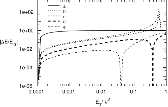
As an example, we calculate the bound-state energy when the coupling is fixed at λ0=100subscript𝜆0100\lambda_{0}=100 to give E0=1subscript𝐸01E_{0}=1. In Fig. 3 we show the ‘errors’ in the binding energy using the same approximations listed above for the potential. As expected, all error lines drop abruptly to zero when λλ0𝜆subscript𝜆0\lambda\rightarrow\lambda_{0}, where the running coupling is chosen to fit what we define to be the exact binding energy. Away from this point we can analyze the errors. With the hamiltonian (a) (unrenormalized) we obtain a dominant error that scales like ln(λ0/λ)lnsubscript𝜆0𝜆{\rm ln}\left(\lambda_{0}/\lambda\right), corresponding to the leading order error. With the renormalized hamiltonian (b) the dominant errors scale like [ln(λ0/λ)]2superscriptdelimited-[]lnsubscript𝜆0𝜆2[{\rm ln}\left(\lambda_{0}/\lambda\right)]^{-2}, indicating the elimination of the leading order logarithmic errors. With the hamiltonian (c) there is a small shift, but no significant change in the error scaling. The added irrelevant operator may remove errors of order (λ0/λ)2superscriptsubscript𝜆0𝜆2(\lambda_{0}/\lambda)^{2}, but these are smaller than the remaining [ln(λ0/λ)]2superscriptdelimited-[]lnsubscript𝜆0𝜆2[{\rm ln}\left(\lambda_{0}/\lambda\right)]^{-2} errors. With hamiltonians (d) and (e) in the range of intermediate cutoffs (E0<<λ2<<λ02much-less-thansubscript𝐸0superscript𝜆2much-less-thansuperscriptsubscript𝜆02E_{0}<<\lambda^{2}<<\lambda_{0}^{2}) there is also only a shift in the errors. The dips in (d) and (e) correspond to values of λ𝜆\lambda where the binding energy equals the exact value.
Refer to caption

Figure 3: The SRG errors in the binding energy for the two-dimensional delta-function potential using various approximations for the SRG hamiltonian. The exact theory is fixed by choosing E0=1subscript𝐸01E_{0}=1 at λ0=100subscript𝜆0100\lambda_{0}=100.

This behavior is a perturbative artifact that can be understood in the following way. Consider the Schrödinger equation with potential (d). Rescaling the momenta pλp~𝑝𝜆~𝑝p\rightarrow\lambda{\tilde{p}} we obtain

p~2Φ~(p~)αλ,42π0𝑑q~q~e(p~2q~2)Φ~(q~)=Eλλ2Φ~(p~).superscript~𝑝2~Φ~𝑝subscript𝛼𝜆42𝜋superscriptsubscript0differential-d~𝑞~𝑞superscript𝑒superscript~𝑝2superscript~𝑞2~Φ~𝑞subscript𝐸𝜆superscript𝜆2~Φ~𝑝{\tilde{p}}^{2}{\tilde{\Phi}}({\tilde{p}})-\frac{\alpha_{\lambda,4}}{2\pi}\;\int_{0}^{\infty}\;d{\tilde{q}}\;{\tilde{q}}\;e^{({\tilde{p}}^{2}-{\tilde{q}}^{2})}\;{\tilde{\Phi}}({\tilde{q}})=\frac{E_{\lambda}}{\lambda^{2}}\;{\tilde{\Phi}}({\tilde{p}})\;. (99)

and

Eλ=λ2[0𝑑p~p~(p~2|Φ~(p~)|2)αλ,42π0𝑑p~p~0𝑑q~q~e(p~2q~2)Φ~(p~)Φ~(q~)]0𝑑p~p~|Φ~(p~)|2.subscript𝐸𝜆superscript𝜆2delimited-[]superscriptsubscript0differential-d~𝑝~𝑝superscript~𝑝2superscript~Φ~𝑝2subscript𝛼𝜆42𝜋superscriptsubscript0differential-d~𝑝~𝑝superscriptsubscript0differential-d~𝑞~𝑞superscript𝑒superscript~𝑝2superscript~𝑞2~Φ~𝑝~Φ~𝑞superscriptsubscript0differential-d~𝑝~𝑝superscript~Φ~𝑝2\displaystyle E_{\lambda}=\lambda^{2}\;\frac{\left[\int_{0}^{\infty}\;d{\tilde{p}}\;{\tilde{p}}\;\left({\tilde{p}}^{2}\;|{\tilde{\Phi}}({\tilde{p}})|^{2}\right)-\frac{\alpha_{\lambda,4}}{2\pi}\;\int_{0}^{\infty}\;d{\tilde{p}}\;{\tilde{p}}\;\int_{0}^{\infty}\;d{\tilde{q}}\;{\tilde{q}}\;e^{({\tilde{p}}^{2}-{\tilde{q}}^{2})}\;{\tilde{\Phi}}({\tilde{p}})\;{\tilde{\Phi}}({\tilde{q}})\right]}{\int_{0}^{\infty}\;d{\tilde{p}}\;{\tilde{p}}\;|{\tilde{\Phi}}({\tilde{p}})|^{2}}\;. (100)

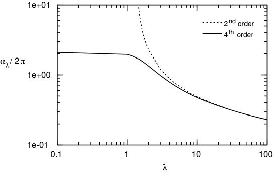
As shown in Fig. 4, the coupling renormalized to fourth-order, αλ,4subscript𝛼𝜆4\alpha_{\lambda,4}, approximately freezes for small λ𝜆\lambda and as a consequence the bound-state energy scales like Eλλ2×constantsimilar-to-or-equalssubscript𝐸𝜆superscript𝜆2constantE_{\lambda}\simeq\lambda^{2}\times{\rm constant} eventually becoming equal to the exact value and then deviating again. With the hamiltonian (e) the behavior is similar, with the dip occurring at a different value of λ𝜆\lambda because of the irrelevant operator. For small values of λ𝜆\lambda the lines converge, indicating the breakdown of the perturbative expansion.
Refer to caption


Figure 4: The SRG running coupling for the two-dimensional delta-function potential obtained with αλ0subscript𝛼subscript𝜆0\alpha_{\lambda_{0}} at λ0=100subscript𝜆0100\lambda_{0}=100 fixed to fit E0=1subscript𝐸01E_{0}=1.

An alternative prescription is to use the potential derived in subsection 5.1 as the starting point for the similarity transformation. We introduce a large momentum cutoff ΛΛ\Lambda, define

αs0=0=αΛ=4πln(1+Λ2E0),subscript𝛼subscript𝑠00subscript𝛼Λ4𝜋ln1superscriptΛ2subscript𝐸0\alpha_{s_{0}=0}=\alpha_{\Lambda}=\frac{4\pi}{{\rm ln}\left(1+\frac{\Lambda^{2}}{E_{0}}\right)}\;, (101)

and set all irrelevant operators to zero at s0=0subscript𝑠00s_{0}=0. Note that the coupling αλ0subscript𝛼subscript𝜆0\alpha_{\lambda_{0}} is fixed at λ0=subscript𝜆0\lambda_{0}=\infty by fitting the exact binding energy. With this definition the similarity hamiltonian with no similarity cutoff becomes well-defined and we can set all of the similarity transformation boundary conditions at s=0𝑠0s=0. The previous derivation remains essentially the same. The only modification is that all integrals over momentum are cut off (pΛ𝑝Λp\leq\Lambda).

At second-order we have

12πdαs,Λds+1(2π)2αs,Λ2dFs,Λ(2)(p,p)ds=αs,Λ2Is,Λ(2)(p,p)12𝜋𝑑subscript𝛼𝑠Λ𝑑𝑠1superscript2𝜋2superscriptsubscript𝛼𝑠Λ2𝑑subscriptsuperscript𝐹2𝑠Λ𝑝superscript𝑝𝑑𝑠superscriptsubscript𝛼𝑠Λ2superscriptsubscript𝐼𝑠Λ2𝑝superscript𝑝-\frac{1}{2\pi}\;\frac{d{\alpha}_{s,\Lambda}}{ds}+\frac{1}{(2\pi)^{2}}\alpha_{s,\Lambda}^{2}\;\frac{dF^{(2)}_{s,\Lambda}(p,p^{\prime})}{ds}=-\alpha_{s,\Lambda}^{2}\;I_{s,\Lambda}^{(2)}(p,p^{\prime}) (102)

where

Is,Λ(2)(p,p)superscriptsubscript𝐼𝑠Λ2𝑝superscript𝑝\displaystyle I_{s,\Lambda}^{(2)}(p,p^{\prime}) =\displaystyle= 1(2π)20Λ𝑑kk(2k2p2p2)e2s[p2p2+k4k2(p2+p2)]1superscript2𝜋2superscriptsubscript0Λdifferential-d𝑘𝑘2superscript𝑘2superscript𝑝2superscript𝑝2superscript𝑒2𝑠delimited-[]superscript𝑝2superscript𝑝2superscript𝑘4superscript𝑘2superscript𝑝2superscript𝑝2\displaystyle\frac{1}{(2\pi)^{2}}\;\int_{0}^{\Lambda}dk\;k\;(2k^{2}-p^{2}-p^{\prime 2})\;e^{-2s[p^{2}p^{\prime 2}+k^{4}-k^{2}(p^{2}+p^{\prime 2})]} (103)
=\displaystyle= 1(2π)2e2sp2p24s.1superscript2𝜋2superscript𝑒2𝑠superscript𝑝2superscript𝑝24𝑠\displaystyle\frac{1}{(2\pi)^{2}}\;\frac{e^{-2s\;p^{2}p^{\prime 2}}}{4s}\;.

The resulting second-order running coupling and irrelevant operator are given respectively by

αs,Λ,2=αΛ1αΛ8π[γ+ln(2sΛ4)Ei(2sΛ4)]subscript𝛼𝑠Λ2subscript𝛼Λ1subscript𝛼Λ8𝜋delimited-[]𝛾ln2𝑠superscriptΛ4Ei2𝑠superscriptΛ4\alpha_{s,\Lambda,2}=\frac{\alpha_{\Lambda}}{1-\frac{\alpha_{\Lambda}}{8\pi}\;\left[\gamma+{\rm ln}\left(2s\Lambda^{4}\right)-{\rm Ei}\left(-2s\Lambda^{4}\right)\right]} (104)

and

Fs,Λ(2)(p,p)subscriptsuperscript𝐹2𝑠Λ𝑝superscript𝑝\displaystyle F^{(2)}_{s,\Lambda}(p,p^{\prime}) =\displaystyle= 14[γ+ln(2sp2p2)Ei(2sp2p2)]14delimited-[]𝛾ln2𝑠superscript𝑝2superscript𝑝2Ei2𝑠superscript𝑝2superscript𝑝2\displaystyle\frac{1}{4}\left[\gamma+{\rm ln}(2s\;p^{2}\;p^{\prime 2})-{\rm Ei}(-2s\;p^{2}\;p^{\prime 2})\right] (105)
+\displaystyle+ 14[γ+ln(2sΛ4)Ei(2sΛ4)]14delimited-[]𝛾ln2𝑠superscriptΛ4Ei2𝑠superscriptΛ4\displaystyle\frac{1}{4}\left[\gamma+{\rm ln}(2s\Lambda^{4})-{\rm Ei}(-2s\Lambda^{4})\right]
\displaystyle- 14[γ+ln(s[(p2Λ2)2+(p2Λ2)2(p2p2)2])\displaystyle\frac{1}{4}\left[\gamma+{\rm ln}\left(s\left[(p^{2}-\Lambda^{2})^{2}+(p^{\prime 2}-\Lambda^{2})^{2}-(p^{2}-p^{\prime 2})^{2}\right]\right)\right.
Ei(s[(p2Λ2)2+(p2Λ2)2(p2p2)2])].\displaystyle\left.\;\;\;\;\;-{\rm Ei}\left(-s\left[(p^{2}-\Lambda^{2})^{2}+(p^{\prime 2}-\Lambda^{2})^{2}-(p^{2}-p^{\prime 2})^{2}\right]\right)\right]\;.

At third-order we have

12πdαs,Λds12𝜋𝑑subscript𝛼𝑠Λ𝑑𝑠\displaystyle-\frac{1}{2\pi}\;\frac{d{\alpha}_{s,\Lambda}}{ds} +\displaystyle+ 1(2π)2αs,Λ2dFs,Λ(2)(p,p)ds+2(2π)2αs,Λdαs,ΛdsFs,Λ(2)(p,p)1superscript2𝜋2superscriptsubscript𝛼𝑠Λ2𝑑subscriptsuperscript𝐹2𝑠Λ𝑝superscript𝑝𝑑𝑠2superscript2𝜋2subscript𝛼𝑠Λ𝑑subscript𝛼𝑠Λ𝑑𝑠subscriptsuperscript𝐹2𝑠Λ𝑝superscript𝑝\displaystyle\frac{1}{(2\pi)^{2}}\;\alpha_{s,\Lambda}^{2}\;\frac{dF^{(2)}_{s,\Lambda}(p,p^{\prime})}{ds}+\frac{2}{(2\pi)^{2}}\;\alpha_{s,\Lambda}\;\frac{d\alpha_{s,\Lambda}}{ds}\;F^{(2)}_{s,\Lambda}(p,p^{\prime}) (106)
+\displaystyle+ 1(2π)3αs,Λ3dFs,Λ(3)(p,p)ds=αs,Λ2Is,Λ(2)(p,p)+αs,Λ3Is,Λ(3)(p,p),1superscript2𝜋3superscriptsubscript𝛼𝑠Λ3𝑑subscriptsuperscript𝐹3𝑠Λ𝑝superscript𝑝𝑑𝑠superscriptsubscript𝛼𝑠Λ2superscriptsubscript𝐼𝑠Λ2𝑝superscript𝑝superscriptsubscript𝛼𝑠Λ3superscriptsubscript𝐼𝑠Λ3𝑝superscript𝑝\displaystyle\frac{1}{(2\pi)^{3}}\;\alpha_{s,\Lambda}^{3}\;\frac{dF^{(3)}_{s,\Lambda}(p,p^{\prime})}{ds}=-\alpha_{s,\Lambda}^{2}\;I_{s,\Lambda}^{(2)}(p,p^{\prime})+\alpha_{s,\Lambda}^{3}\;I_{s,\Lambda}^{(3)}(p,p^{\prime})\;,

where

Is,Λ(3)(p,p)superscriptsubscript𝐼𝑠Λ3𝑝superscript𝑝\displaystyle I_{s,\Lambda}^{(3)}(p,p^{\prime}) =\displaystyle= 1(2π)30Λ𝑑kk(2k2p2p2)e2s[p2p2+k4k2(p2+p2)]1superscript2𝜋3superscriptsubscript0Λdifferential-d𝑘𝑘2superscript𝑘2superscript𝑝2superscript𝑝2superscript𝑒2𝑠delimited-[]superscript𝑝2superscript𝑝2superscript𝑘4superscript𝑘2superscript𝑝2superscript𝑝2\displaystyle\frac{1}{(2\pi)^{3}}\;\int_{0}^{\Lambda}dk\;k\;(2k^{2}-p^{2}-p^{\prime 2})\;e^{-2s[p^{2}p^{\prime 2}+k^{4}-k^{2}(p^{2}+p^{\prime 2})]} (107)
×\displaystyle\times [Fs(2)(p,k)+Fs(2)(k,p)].delimited-[]subscriptsuperscript𝐹2𝑠𝑝𝑘subscriptsuperscript𝐹2𝑠𝑘superscript𝑝\displaystyle\left[F^{(2)}_{s}(p,k)+F^{(2)}_{s}(k,p^{\prime})\right]\;.

In this case,

Fs,Λ(2)(0,k)subscriptsuperscript𝐹2𝑠Λ0𝑘\displaystyle F^{(2)}_{s,\Lambda}(0,k) =\displaystyle= 14[γ+ln(2sΛ4)Ei(2sΛ4)]14delimited-[]𝛾ln2𝑠superscriptΛ4Ei2𝑠superscriptΛ4\displaystyle\frac{1}{4}\left[\gamma+{\rm ln}(2s\Lambda^{4})-{\rm Ei}(-2s\Lambda^{4})\right] (108)
=\displaystyle= 14[γ+ln(2sΛ42sk2Λ2)Ei(2sΛ4+2sk2Λ2)],14delimited-[]𝛾ln2𝑠superscriptΛ42𝑠superscript𝑘2superscriptΛ2Ei2𝑠superscriptΛ42𝑠superscript𝑘2superscriptΛ2\displaystyle\frac{1}{4}\left[\gamma+{\rm ln}(2s\Lambda^{4}-2sk^{2}\Lambda^{2})-{\rm Ei}(-2s\Lambda^{4}+2sk^{2}\Lambda^{2})\right]\;,

and so

Is,Λ(3)(0,0)superscriptsubscript𝐼𝑠Λ300\displaystyle I_{s,\Lambda}^{(3)}(0,0) =\displaystyle= 1(2π)3140Λdk 4k3e2sk4([γ+ln(2sΛ4)Ei(2sΛ4)]\displaystyle\frac{1}{(2\pi)^{3}}\;\frac{1}{4}\;\int_{0}^{\Lambda}dk\;4k^{3}e^{-2sk^{4}}\;\left(\left[\gamma+{\rm ln}(2s\Lambda^{4})-{\rm Ei}(-2s\Lambda^{4})\right]\right. (109)
\displaystyle- [γ+ln(2sΛ42sk2Λ2)Ei(2sΛ4+2sk2Λ2)]).\displaystyle\left.\left[\gamma+{\rm ln}(2s\Lambda^{4}-2sk^{2}\Lambda^{2})-{\rm Ei}(-2s\Lambda^{4}+2sk^{2}\Lambda^{2})\right]\right)\;.

Since Is,Λ(3)(0,0)0superscriptsubscript𝐼𝑠Λ3000I_{s,\Lambda}^{(3)}(0,0)\neq 0 the term proportional to αs,Λ3superscriptsubscript𝛼𝑠Λ3\alpha_{s,\Lambda}^{3} in Eq. (85) does not vanish. To obtain αs,Λ,3subscript𝛼𝑠Λ3\alpha_{s,\Lambda,3} we evaluate Is,Λ(3)(0,0)superscriptsubscript𝐼𝑠Λ300I_{s,\Lambda}^{(3)}(0,0) and solve Eq. (85) numerically.

The equation for Fs,Λ(3)(p,p)subscriptsuperscript𝐹3𝑠Λ𝑝superscript𝑝F^{(3)}_{s,\Lambda}(p,p^{\prime}) is given by

1(2π)3dFs,Λ(3)(p,p)ds=1πIs,Λ(2)(0,0)Fs,λ(2)(p,p)+Is,Λ(3)(p,p).1superscript2𝜋3𝑑subscriptsuperscript𝐹3𝑠Λ𝑝superscript𝑝𝑑𝑠1𝜋superscriptsubscript𝐼𝑠Λ200subscriptsuperscript𝐹2𝑠𝜆𝑝superscript𝑝superscriptsubscript𝐼𝑠Λ3𝑝superscript𝑝\frac{1}{(2\pi)^{3}}\frac{dF^{(3)}_{s,\Lambda}(p,p^{\prime})}{ds}=-\frac{1}{\pi}\;I_{s,\Lambda}^{(2)}(0,0)\;F^{(2)}_{s,\lambda}(p,p^{\prime})+I_{s,\Lambda}^{(3)}(p,p^{\prime})\;. (110)

To obtain Fs,Λ(3)(p,p)subscriptsuperscript𝐹3𝑠Λ𝑝superscript𝑝F^{(3)}_{s,\Lambda}(p,p^{\prime}) the integrals over k𝑘k and s𝑠s must be evaluated numerically. In the limit sΛ4𝑠superscriptΛ4s\Lambda^{4}\rightarrow\infty with s𝑠s fixed at some non-zero value

Fs,Λ(2)(p,p)14[γ+ln(2sp2p2)Ei(2sp2p2)],subscriptsuperscript𝐹2𝑠Λ𝑝superscript𝑝14delimited-[]𝛾ln2𝑠superscript𝑝2superscript𝑝2Ei2𝑠superscript𝑝2superscript𝑝2\displaystyle F^{(2)}_{s,\Lambda}(p,p^{\prime})\rightarrow\frac{1}{4}\left[\gamma+{\rm ln}(2s\;p^{2}\;p^{\prime 2})-{\rm Ei}(-2s\;p^{2}\;p^{\prime 2})\right]\;, (111)
Is,Λ(3)(0,0)0,superscriptsubscript𝐼𝑠Λ3000\displaystyle I_{s,\Lambda}^{(3)}(0,0)\rightarrow 0\;, (112)

and αs,Λsubscript𝛼𝑠Λ\alpha_{s,\Lambda} becomes indeterminate, requiring the coupling to be fixed at some s00subscript𝑠00s_{0}\neq 0. In this way, we recover the result of the previous prescription.

Although less trivial, this prescription allows a more transparent error analysis. We can also extend the calculation to larger values of the similarity cutoff, λ𝜆\lambda, and analyze the errors in a different scaling regime. In Fig. 5 we show the errors in the binding-energy obtained using the following approximations for the potential with Λ=50Λ50\Lambda=50:

(a) marginal operator with coupling (αλ0subscript𝛼subscript𝜆0\alpha_{\lambda_{0}}),

Vλ,Λ(p,p)=αΛ2πe(p2p2)2λ4;subscript𝑉𝜆Λ𝑝superscript𝑝subscript𝛼Λ2𝜋superscript𝑒superscriptsuperscript𝑝2superscript𝑝22superscript𝜆4V_{\lambda,\Lambda}(p,p^{\prime})=-\frac{\alpha_{\Lambda}}{2\pi}\;e^{-\frac{(p^{2}-p^{\prime 2})^{2}}{\lambda^{4}}}\;; (113)

(b) marginal operator with running coupling renormalized to second-order (αλ,Λ,2subscript𝛼𝜆Λ2\alpha_{\lambda,\Lambda,2}),

Vλ,Λ(p,p)=αλ,Λ,22πe(p2p2)2λ4;subscript𝑉𝜆Λ𝑝superscript𝑝subscript𝛼𝜆Λ22𝜋superscript𝑒superscriptsuperscript𝑝2superscript𝑝22superscript𝜆4V_{\lambda,\Lambda}(p,p^{\prime})=-\frac{\alpha_{\lambda,\Lambda,2}}{2\pi}\;e^{-\frac{(p^{2}-p^{\prime 2})^{2}}{\lambda^{4}}}\;; (114)

(c) marginal operator plus second-order irrelevant operator with running coupling renormalized to second-order (αλ,Λ,2,Fλ(2)subscript𝛼𝜆Λ2subscriptsuperscript𝐹2𝜆\alpha_{\lambda,\Lambda,2},F^{(2)}_{\lambda}),

Vλ,Λ(p,p)=[αλ,Λ,22π+(αλ,Λ,22π)2Fλ,Λ(2)(p,p)]e(p2p2)2λ4;subscript𝑉𝜆Λ𝑝superscript𝑝delimited-[]subscript𝛼𝜆Λ22𝜋superscriptsubscript𝛼𝜆Λ22𝜋2subscriptsuperscript𝐹2𝜆Λ𝑝superscript𝑝superscript𝑒superscriptsuperscript𝑝2superscript𝑝22superscript𝜆4V_{\lambda,\Lambda}(p,p^{\prime})=\left[-\frac{\alpha_{\lambda,\Lambda,2}}{2\pi}+\left(\frac{\alpha_{\lambda,\Lambda,2}}{2\pi}\right)^{2}\;F^{(2)}_{\lambda,\Lambda}(p,p^{\prime})\right]\;e^{-\frac{(p^{2}-p^{\prime 2})^{2}}{\lambda^{4}}}\;; (115)

(d) marginal operator with running coupling renormalized to third-order (αλ,Λ,3subscript𝛼𝜆Λ3\alpha_{\lambda,\Lambda,3}),

Vλ,Λ(p,p)=αλ,Λ,32πe(p2p2)2λ4;subscript𝑉𝜆Λ𝑝superscript𝑝subscript𝛼𝜆Λ32𝜋superscript𝑒superscriptsuperscript𝑝2superscript𝑝22superscript𝜆4V_{\lambda,\Lambda}(p,p^{\prime})=-\frac{\alpha_{\lambda,\Lambda,3}}{2\pi}\;e^{-\frac{(p^{2}-p^{\prime 2})^{2}}{\lambda^{4}}}\;; (116)

(e) marginal operator plus second-order irrelevant operator with running coupling renormalized to third-order αλ,Λ,3,Fλ(2)subscript𝛼𝜆Λ3subscriptsuperscript𝐹2𝜆\alpha_{\lambda,\Lambda,3},F^{(2)}_{\lambda}),

Vλ,Λ(p,p)=[αλ,Λ,32π+(αλ,Λ,32π)2Fλ,Λ(2)(p,p)]e(p2p2)2λ4.subscript𝑉𝜆Λ𝑝superscript𝑝delimited-[]subscript𝛼𝜆Λ32𝜋superscriptsubscript𝛼𝜆Λ32𝜋2subscriptsuperscript𝐹2𝜆Λ𝑝superscript𝑝superscript𝑒superscriptsuperscript𝑝2superscript𝑝22superscript𝜆4V_{\lambda,\Lambda}(p,p^{\prime})=\left[-\frac{\alpha_{\lambda,\Lambda,3}}{2\pi}+\left(\frac{\alpha_{\lambda,\Lambda,3}}{2\pi}\right)^{2}\;F^{(2)}_{\lambda,\Lambda}(p,p^{\prime})\right]\;e^{-\frac{(p^{2}-p^{\prime 2})^{2}}{\lambda^{4}}}\;. (117)

Refer to caption

Figure 5: The SRG errors in the binding energy for the two-dimensional delta-function potential using various approximations for the similarity hamiltonian. The exact theory is fixed by regulating the “bare hamiltonian” using a sharp momentum cutoff, ΛΛ\Lambda, and letting the bare coupling depend on ΛΛ\Lambda such that the binding energy is fixed. We use Λ=50Λ50\Lambda=50 and E0=1subscript𝐸01E_{0}=1.

There are clearly two distinct scaling regions when an additional large momentum cutoff ΛΛ\Lambda is placed on the initial matrix and a similarity cutoff is then applied. When the similarity cutoff is larger than ΛΛ\Lambda, we see power-law improvement resulting from the addition of irrelevant operators. Curves (a), (b), and (d) all have the same slope. None of these hamiltonians contains irrelevant operators, but the marginal coupling differs in each. All results become exact as the similarity cutoff goes to infinity, and these curves are close to one another because the coupling runs little in this region. Curves (c) and (e) show that there is a power-law improvement when irrelevant operators are added, and that once again when the similarity cutoff is larger than ΛΛ\Lambda an improvement in the running coupling makes little difference. Even though the coupling in front of this operator is approximated by the first term in an expansion in powers of the running coupling, the coupling is sufficiently small that this approximation works well and the operator eliminates most of the leading power-law error in curves (a), (b), and (d).

When the similarity cutoff become smaller than ΛΛ\Lambda we see a crossover to a more complicated scaling regime that resembles the SRG scaling discussed above. The error displayed by curve (a) approaches 100%, while the running coupling introduced in curve (b) reduces the error to an inverse logarithm. Improving the running coupling in curve (d) further reduces the error, and we see that curve (c) crosses curve (d) at a point where improving the running coupling becomes more important than adding irrelevant operators. As above, the best results require us to both improve the running coupling by adding third-order corrections and add the second-order irrelevant operators. In no case do we achieve power-law improvement, because as we have discussed there are always residual inverse logarithmic errors. Had we fit the running coupling to data, as we would do in a realistic calculation, we would obtain power-law improvement and the residual error would be proportional to an inverse power of the cutoff times an inverse power of the logarithm of the cutoff.

In Fig. 6 we show the running coupling at 2nd and 3rd order. Although the 3rd order corrections are small for all λ𝜆\lambda and vanish when ΛΛ\Lambda\rightarrow\infty, the improvement resulting from this correction in Fig. 5 is significant.
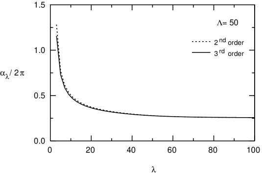
Refer to caption

Figure 6: The SRG running coupling for the two-dimensional delta-function potential renormalized to second and third-order obtained with αλ0=αΛ=4π/ln(1+Λ2E0)subscript𝛼subscript𝜆0subscript𝛼Λ4𝜋ln1superscriptΛ2subscript𝐸0\alpha_{\lambda_{0}=\infty}\rightarrow\alpha_{\Lambda}=4\pi/{\rm ln}\left(1+\frac{\Lambda^{2}}{E_{0}}\right).

The scaling behavior with a large momentum cutoff ΛΛ\Lambda in place is complicated, but it is fairly straightforward to understand it and to find a sequence of approximations that systematically improve the non-perturbative results. The calculations become increasingly complicated, but at each order one must improve the running coupling, or fit it to data, and add higher order irrelevant operators. In a field theory we need to let ΛΛ\Lambda\rightarrow\infty and study the scaling behavior of the theory in the regime where λΛmuch-less-than𝜆Λ\lambda\ll\Lambda. Although we do not display a compete set of figures, in Fig. 7 we show what happens to the running coupling as ΛΛ\Lambda is increased, with the bound state energy fixed at one.
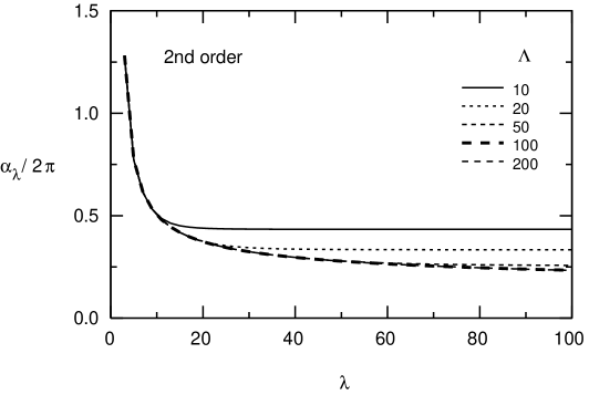
Refer to caption

Figure 7: The SRG running coupling for the two-dimensional delta-function potential renormalized to second-order obtained with αλ0=αΛ=4π/ln(1+Λ2E0)subscript𝛼subscript𝜆0subscript𝛼Λ4𝜋ln1superscriptΛ2subscript𝐸0\alpha_{\lambda_{0}=\infty}\rightarrow\alpha_{\Lambda}=4\pi/{\rm ln}\left(1+\frac{\Lambda^{2}}{E_{0}}\right).

As is evident in the exact solution, as ΛΛ\Lambda increases the coupling decreases. When λΛmuch-greater-than𝜆Λ\lambda\gg\Lambda, the coupling runs slowly and stays near its asymptotic value. As λ𝜆\lambda approaches ΛΛ\Lambda the coupling begins to run noticeably, and when λ𝜆\lambda becomes much less than ΛΛ\Lambda the coupling approaches a universal curve that is insensitive to its asymptotic value. Plots of the error in the binding energy for various approximations and different values of ΛΛ\Lambda closely resemble Fig. 11, with two scaling regimes whose boundary is λ=Λ𝜆Λ\lambda=\Lambda.

We close this section by reminding the reader that in all of these calculations there is only one free parameter. In a realistic calculation we would fit this parameter to a binding energy and we would expect to see residual errors in other observables that is inversely proportional to powers of the cutoff and logarithms of the cutoff.

4 Conclusions

We have illustrated the similarity renormalization group method for producing effective cutoff hamiltonians using the two-dimensional delta-function potential. We have shown that the SRG with coupling coherence leads to errors that scale as inverse powers of the cutoff and inverse logarithms of the cutoff. The SRG with coupling coherence requires the same number of parameters as the underlying ‘fundamental’ theory, but the cost is exponentially increasing algebraic complexity to remove errors that contain inverse powers of logarithms of the cutoff.

5 Acknowledgments

We would like to acknowledge many useful discussions with Brent Allen, Martina Brisudova, Dick Furnstahl, Stan Głazek, Billy Jones, Roger Kylin, Rick Mohr, Jim Steele, and Ken Wilson. This work was supported by National Science Foundation grant PHY-9800964, and S.S. was supported by a CNPq-Brazil fellowship (proc. 204790/88-3).

References

  • [1] J. Schwinger, “Quantum Electrodynamics,” Dover, New York, 1958.
  • [2] P. A. M. Dirac, Theorie du Positron, (7-eme Conseil du Physique du Solvay: Structure et propiete de noyaux atomiques, Octobre 1933), pp. 203-230, Gauthier-Villars, Paris, 1934.
  • [3] P.A.M. Dirac, in “Perturbative Quantum Chromodynamics,” (D.W. Duke and J.F. Owens, Eds.), Am. Inst. Phys., New York, 1981.
  • [4] E. C. G. Stueckelberg and A. Peterman, Helv. Phys. Acta 26 (1953), 499.
  • [5] M. Gell-Mann and F.E. Low, Phys. Rev. 95 (1954), 1300.
  • [6] L. D. Landau, A. A. Abrikosov and I. M. Khalatnikov, Doklady 95 (1954), 497; 96 (1954), 261.
  • [7] N. N. Bogoliubov and D.V. Shirkov, Nuovo Cim. 3 (1956), 845.
  • [8] N. N. Bogoliubov and D.V. Shirkov, “Introduction to the Theory of Quantized Fields,” Interscience, New York, 1959.
  • [9] K. G. Wilson and J. B. Kogut, Phys. Rep. 12C (1974), 75.
  • [10] K. G. Wilson, Rev. Mod. Phys. 47 (1975), 773.
  • [11] D. J. Gross and F. Wilczek, Phys. Rev. Lett. 30 (1973), 1343;
    H. D. Politzer, Phys. Rev. Lett. 30 (1973), 1346.
  • [12] Ya. B. Zel’dovich, Soviet Physics JETP 11 (1960), 594.
  • [13] F. A. Berezin and L. D. Faddeev, Sov. Math. Dokl. 2 (1961), 372.
  • [14] C. Thorn, Phys. Rev. D 19 (1979), 639.
  • [15] K. Huang, “Quarks, Leptons and Gauge Fields,” World Scientific, Singapore, 1982.
  • [16] S. Albeverio, F. Gesztesy, R. Hoeg-Krohn and H. Holden, “Solvable Models in Quantum mechanics,” Springer-Verlag, New York, 1988.
  • [17] C. R. Hagen, Phys. Rev. Lett. 64 1990), 503.
  • [18] R. Jackiw, in “M. A. B. Beg Memorial Volume,” (A. Ali and P. Hoodbhoy, eds.), World Scientific, Singapore, 1991.
  • [19] P. Godsdzinky and R. Tarrach, Am. J. Phys. 59 (1991), 70;
    C. Manuel and R. Tarrach, Phys. Lett. B 328 (1994), 113.
  • [20] J. F. Perez and F. A. B. Coutinho, Am. J. Phys. 59 (1991), 52.
  • [21] L. R. Mead and J. Godines, Am. J. Phys. 59 (1991), 935.
  • [22] C. Manuel and R. Tarrach, Phys. Lett. B 301 (1994), 72.
  • [23] T. J. Fields, K. S. Gupta, and J. P. Vary, Mod. Phys. Lett. A 11 (1996), 2233.
  • [24] K. S. Gupta and S. G. Rajeev, Phys. Rev. D 48 (1993), 5940;
    R. J. Henderson and S. G. Rajeev, Intl. J. Mod. Phys. A 10 (1995), 3765;
    R. J. Henderson and S. G. Rajeev, J. Math. Phys. 38 (1997), 2171.
  • [25] D. K. Park, J. Math. Phys. 36 (1995), 5453.
  • [26] S. K. Adhikari and T. Frederico, Phys. Rev. Lett. 74 (1995), 4572;
    S. K. Adhikari, T. Frederico and I. D. Goldman, Phys. Rev. Lett. 74 (1995), 487;
    S. K. Adhikari and A. Ghosh, J. Phys. A 30 (1997), 6553;
    C. F. de Araujo, Jr., L. Tomio, S. K. Adhikari and T. Frederico, J. Phys A 30 (1997), 4687.
  • [27] R. M. Cavalcanti, quant-ph/9801033 (1998).
  • [28] R. J. Henderson and S. G. Rajeev, J. Math. Phys. 39 (1998), 749.
  • [29] D. R. Phillips, S. R. Beane, and T. D. Cohen, Ann. Phys. (N.Y.) 263 (1998), 255.
  • [30] S. D. Głazek and K.G. Wilson, Phys. Rev. D 48 (1993), 5863.
  • [31] S. D. Głazek and K.G. Wilson, Phys. Rev. D 49 (1994), 4214.
  • [32] F. Wegner, Ann. Physik (Berlin) 3 (1994), 77.
  • [33] K. G. Wilson, Phys. Rev. 140 (1965), B445.
  • [34] K. G. Wilson, Phys. Rev. D2 (1970), 1438.
  • [35] C. Bloch, Nucl. Phys. 6 (1958), 329.
  • [36] R. Oehme and W. Zimmermann, Commun. Math. Phys. 97 (1985), 569;
    R. Oehme, K. Sibold and W. Zimmermann, Phys. Lett. B 147 (1984), 115.
  • [37] R. J. Perry and K. G. Wilson, Nucl. Phys. B 403 (1993), 587;
    R. J. Perry, Ann. Phys. (N.Y.) 232 (1994), 116.
  • [38] S. Coleman and E. Weinberg, Physical Review D 7 (1973), 1888.