Two dimensional $CP^{2}$ Model with $\theta$-term and Topological Charge Distributions

1 Introduction

Quantum Chromodynamics(QCD) admits the topological term, i.e., $\theta$-term. It leads to “strong CP violation”. Experimentally, the magnitude of $\theta$ parameter which controls the magnitude of strong CP violation is severely limited to a tiny value( $|\theta|\mathrel{\hbox{\raise 0.86108pt\hbox{$<$}\kern-7.5pt\raise-3.87495pt\hbox{$\sim$}}}10^{-9}$). Lattice gauge theory( LGT), formulated by K.G. Wilson[1] and developed by M.Creutz[2], has made a realistic progress in understanding the nature of QCD. In LGT in which Euclidean space-time is adopted, usual gauge coupling is purely real quantity. On the other hand, $\theta$-term appears as a purely imaginary quantity. Combining both of these leads to complex numbered coupling. The action given by this complex coupling constant gives complex valued Boltzmann weight. Except for a few number of cases, the works in LGT are done for real couplings. It is, however, very important to understand the role of complex coupling cases, i.e., the system with $\theta$-term. Monte Carlo simulations are confronted with a difficulty due to complex Boltzmann weight. Monte Carlo simulation in this case was made possible to some extent by Bhanot et al. [3][4], Wiese [5] and Karliner et al.[6][7].

The method is summarized as follows; 1)First we obtain the topological charge [8] distribution $P(Q)$ with the use of the Boltzmann weight defined by the real coupling constant. Fourier series

$$Z(\theta)=\sum_{Q}P(Q)e^{i\theta Q}$$

gives the partition function $Z(\theta)$ for the system with $\theta$-term.

2) There are some technical problems to obtain topological charge distribution. Since the topological charge distribution is a rapidly decreasing function, we use (i) “set method”, in which the whole range of $Q$ is divided into number of sets. In each set, MC simulation is performed. (ii)even after dividing into sets, the distribution is still rapidly decreasing, so we use “trial distribution method”, in which the Boltzmann weight is normalized by some appropriate trial function so as to realize the slowly changing topological charge distribution. This method was applied to 2 dimensional U(1) system with $\theta$-term . Wiese showed that the first order phase transition is observed at $\theta=\pi$ for all real couplings [5].

Two dimensional $CP^{N-1}$ system has many qualitative similarity with 4 dimensional QCD, like, asymptotic freedom, confinement, deconfinement phase( Higgs phase) and topological excitations( instanton).

Schierholz studied 2 dimensional $CP^{3}$ system with $\theta$-term[9]. He observed that,

1)in strong couplings, the first order phase transition occurs at a critical value $\theta_{c}=\pi$ and that

2)in weak couplings, deviation of the position of the first order transition from $\theta_{c}=\pi$ to smaller values. He conjectured that $\theta_{c}\rightarrow 0$ as $\beta\rightarrow\infty$( weak coupling limit) and that the continuum limit value of $\theta$ is zero.

If this conjecture is valid, it gives quite important physical result, but almost no confirmation is made by other groups. One of the aim of the present paper is to investigate this issue [10].

We will briefly summarize the approach other than MC. We analyzed 2 dimensional U(1) system with $\theta$-term [11] based on the group character expansion method [12]. Topological charge distribution $P(Q)$ is shown to be given by a Gaussian function $\exp(-\kappa_{V}Q^{2}))$ for all $\beta$. It leads to the result that the partition function is given by the third elliptic theta function $\vartheta_{3}(\nu,\tau)$. It has a remarkable property that the partition function has an infinite numbers of zeros as a function of $z=e^{i\theta}$, where $\theta$ is extended to complex values. In infinite volume limit, these infinite numbers of partition function zeros accumulate to $z=-1$ according to $\kappa_{V}\propto 1/V$. Namely, first order phase transition is expected at $\theta=\pi$ in the limit $V\rightarrow\infty$, where $V=L^{2}$ denotes the volume of system.

Four dimensional $Z_{N}$ gauge system with $\theta$-term is discussed by Cardy and Rabinovici [13]. They pointed out that $\theta$-term leads to symmetries under dual transformation of Hamiltonian and this symmetry leads to very rich phase structures, namely, confinement phase, Higgs phase( deconfinement phase) and condensation of electric and magnetic charges( oblique confinement) [14]. Their argument is based on free energy and rather qualitative. It will be of much interest to investigate this system by MC simulation or other method( e.g., renormalization group method).

In the previous paper [15], we performed MC simulation on $CP^{1}$ system with $\theta$-term in strong and weak coupling regions. In strong coupling regions, first order phase transition is observed at $\theta=\pi$ [16][17]. In weak coupling regions [18], we observed that topological charge distribution deviates apparently from Gaussian form. Free energy in weak coupling regions is approximately given by $\cos\theta$ form, which shows only a few small $Q$’s control the topological charge distribution. In intermediate coupling regions, obtained results were not so clear. In order to avoid the effect of statistical error as far as possible, we used fitted analytic form for $P(Q)$ to obtain $Z(\theta),F(\theta)$ etc. Then even in weak coupling region we observed no flattening behavior but change of behavior of $Z(\theta),F(\theta)$. The power series fit to $P(Q)$ has the property;

1)for $\beta$ small( strong coupling regions), it is simply given by Gaussian form( $\exp(-\kappa_{V}Q^{2}))$.

2)for $\beta$ large( weak coupling regions), we need $Q^{4}$ term in the polynomial fit of the exponent of $P(Q)$.

3)for $\beta$ intermediate, power series fit suffers from quite large $\chi^{2}$ value.

In this paper, CP² model with $\theta$-term will be studied by MC method [19]. The emphasis is put on intermediate coupling regions($\beta=3\sim 4$). From $P(Q)$ we obtain $Z(\theta)$ and we obtain free energy per unit volume by $F(\theta)=-(1/V)\ln Z(\theta)$. $F(\theta)$ grows smoothly in smaller $\theta$ and shows “flattening” at some value $\theta_{f}$, beyond which $F(\theta)$ becomes almost flat. For example, at $\beta=3.5$ and $\ L=20$( 100000=100 kiro iterations), flattening is observed at $\theta=\theta_{f}\sim 0.57\pi$. Does it correspond to the “first order phase transition” found by Schierholz in CP³ system?

Does the flattening mentioned above really mean a phase transition? We should be careful about the statistical error induced by the simulation. For example, after $N$ times of sweeps( =iterations), we would have statistical error of order

$$\delta P=|{\rm error}|\sim 1/\sqrt{N}.$$

Note that $\delta P$ is defined as positive.

Set method and trial function method will give us $P(Q)$ containing great number of orders of decrease from $Q=0$ to large value of $Q$. If observed $P(Q)$ is fitted by a smooth function $P_{S}(Q)$, it can be expressed as,

$$P(Q)=P_{S}(Q)+\mathchar 28929\relax P(Q),$$

where $\mathchar 28929\relax P(Q)$ is the difference between observed $P(Q)$ and the fitted function $P_{S}(Q)$. Quantity $|\mathchar 28929\relax P(Q)|$ will be approximately given by $\delta P\times P(Q)$. The quantity $\mathchar 28929\relax P(Q)$ can be both positive and negative( or zero), since it is a fluctuation. The value of $|\mathchar 28929\relax P(Q)|$ is approximately of order of $(1/\sqrt{N})P(Q)$ and $\mathchar 28929\relax P(Q)$ itself is expected to be small at large $Q$. Partition function $Z(\theta)$, however, is given by the fourier series and the error in evaluation of $Z(\theta)$ is controlled by the largest one, i.e., $|\mathchar 28929\relax P(0)|\sim\delta P\sim 1/\sqrt{N}$. Topological charge distribution $P(Q)$ is a rapidly decreasing function. When we estimate $Z(\theta)$ from

$$Z(\theta)=\sum_{Q}P(Q)e^{i\theta Q},$$

the value of $Z(\theta)$ will also be a rapidly decreasing function of $\theta$ and the quantity $\mathchar 28929\relax P(0)$ will play an important role at large $\theta$. Since the partition function obtained by $P_{S}(Q)$ is a rapidly decreasing function, true $Z_{S}(\theta)$ will be masked by the error $\mathchar 28929\relax P(0)$ at large $\theta$, which is much larger than $P_{S}(Q)$ itself at large $Q$ . This effect leads to the shape of $Z(\theta)$ with flattening at some $\theta_{f}$ just like the illustration shown in Fig.1($\theta_{f}\sim 0.55\pi$ in this figure).

Fig. 1: An illustration of partition function as a function of theta. Direct fourier series( curve with flattening behavior) and one( Gaussian curve) calculated from smooth fit to $P(Q)$.

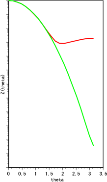
The value of $Z(\theta)$ will almost coincide with $Z_{S}(\theta)$ in $\theta<\theta_{f}$ but it deviates far from $Z(\theta)_{S}$ in $\theta\mathrel{\hbox{\raise 0.86108pt\hbox{$>$}\kern-7.5pt\raise-3.87495pt\hbox{$\sim$}}}\theta_{f}$. $Z_{S}(\theta)$ will become quite small as $\theta\rightarrow\pi$ but obtained $Z(\theta)$ does not show such suppression.

In this way the combined method of set and trial function leads to satisfactory result for $P(Q)$ but we still encounter difficulty in obtaining correct $Z(\theta)$ at large $\theta$’s.

In order to confirm the physical flattening (if it exists), we need enough accuracy of $Z(\theta)$ over huge range of magnitude. For example to confirm the behavior of partition function down to 10^-8, we need $N\sim 10^{16}$ iterations.

To obtain information about flattening within available computer facilities, we should analyze at larger $\beta$ or smaller volume $V$, since $P(Q)$ decreases faster at $\beta=$ large or at $V=$ small, partition function $Z(\theta)$, which is a Fourier transform of $P(Q)$, falls slowly at $\beta=$ large or $V=$ small. In these regions $Z(\theta)$ will be reliably estimated over whole region of $\theta(0\leq\theta\leq\pi$).

2 $CP^{2}$ model in two dimensions

2.1 $CP^{2}$ model in two dimensions

We define the $CP^{2}$ model with $\theta$-term in the two dimensional euclidean lattice space. The $CP^{2}$ model consists of three component complex scalar fields,

$$z_{\alpha}(n)=\left(\begin{array}[]{c}z_{1}(n)\\ z_{2}(n)\\ z_{3}(n)\\ \end{array}\right),$$ (2.4)

at each site $n$, and constrained by

$$\sum_{\alpha=1}^{3}z_{\alpha}^{\ast}(n)z_{\alpha}(n)=1.$$ (2.5)

Action, which is U(1) gauge invariant, is given by

$$S_{\theta}[z] = S[z]-i\theta Q[z]$$ (2.6)

$$S = \beta\sum_{n=1}^{L^{2}}\sum_{\mu=1,2}\{1-\sum_{\alpha=1}^{3}{|z_{\alpha}^{\ast}(n)z_{\alpha}(n+\mu)|}^{2}\},$$ (2.7)

where $Q$ is topological charge, and $z_{\alpha}(n)$ is coupled with $z_{\alpha}(n+\mu)$ at the nearest neighbor site $n+\mu(\mu=1,2)$. Topological charge $Q$ is defined by

$$Q = \frac{1}{4\pi}\sum_{plaq}\epsilon_{\mu\nu}(A_{\mu}(n)+A_{\nu}(n+\mu)-A_{\mu}(n+\nu)-A_{\nu}(n))$$ (2.8)

where, $A_{\mu}(n)=\arg(z^{\ast}(n)z(n+\mu))$. Topological charge $Q$ is given by the winding number, i.e., how often the field $A_{\mu}(n)$ covers $U(1)$ space when we move around the periodic boundary of the whole space time once.

The partition function as a function of the coupling constant $\beta$ and $\theta$ is

$$Z(\theta)=\frac{\int Dz^{\ast}Dz\exp(-S[z]+i\theta Q[z])}{\int Dz^{\ast}Dz\exp(-S[z])}$$ (2.9)

where $Dz$ denotes integration over all fields, and the free energy $F(\theta)$ is given by

$$F(\theta)=-\frac{1}{V}\ln Z(\theta),$$ (2.10)

where $V$ is volume of the lattice space.

We would like to compute $\theta$ vacua effects, but the complex Boltzmann factor $e^{i\theta Q}$ prevents us from performing ordinary Monte Carlo simulation. In order to get over this difficulty, we follow Wiese’s idea. The updating is restricted to the fields in the topological sector. Thus the phase factor $e^{i\theta Q[z]}$ is replaced by a constant and can be factored out from the functional integral. We can perform ordinary Monte Carlo simulation using the real action $S[z]$. The partition function is given by the summation of the topological charge distribution $P(Q)$ weighted by $e^{i\theta Q}$ in each $Q$ sector. In practice, we get the topological charge distribution $P(Q)$ at $\theta=0$ by the Monte Carlo simulation. We obtain the partition function $Z(\theta)$ by taking the Fourier transform of $P(Q)$.

$$Z(\theta) = \sum_{Q}e^{i\theta Q}P(Q)$$ (2.11)

where P(Q) is

$$P(Q) \equiv \frac{\int Dz^{\ast(Q)}Dz^{(Q)}\exp(-S[z])}{\int Dz^{\ast}Dz\exp(-S[z])}$$ (2.12)

The integration measure $Dz^{(Q)}$ is restricted to the fields in the topological sector labeled by the topological charge $Q$. Note that $\sum_{Q}P(Q)=1$.

The expectation value of an observable $O$ is given in terms of $P(Q)$ as

$$\langle O\rangle_{\theta} = \frac{\sum_{Q}P(Q)\ \langle O\rangle_{Q}\ e^{-i\theta Q}}{\sum_{Q}P(Q)\ e^{-i\theta Q}},$$ (2.13)

where $\langle O\rangle_{Q}$ is the expectation value of $O$ at $\theta=0$ for a given $Q$ sector

$$\langle O\rangle_{Q}=\frac{\int Dz^{\ast(Q)}Dz^{(Q)}\ O\ e^{-S[z]}}{\int Dz^{\ast(Q)}Dz^{(Q)}\ e^{-S[z]}}.$$ (2.14)

2.2 Algorithm

We measure the topological charge distribution $P(Q)$ by Monte Carlo simulation with the Boltzmann weight exp($-S$), where $S$ is defined by eq.(2.4). The standard Metropolis method is used to update configurations. To calculate $P(Q)$, we count the number of times the configuration of $Q$ is visited by histogram method. The distribution $P(Q)$ damps very rapidly as $\mid Q\mid$ becomes large. We need to calculate $P(Q)$ at as larger $|Q|$ as possible, which would contribute to $F(\theta),\langle Q\rangle_{\theta}$ and $\langle Q^{2}\rangle_{\theta}$ because they are obtained by Fourier transformation of $P(Q)$ and the derivatives of the partition function by $\theta$. In order to obtain $P(Q)$ at larger $Q$’s, we apply following two techniques,

1. the set method,

2. the trial distribution method.

The set method ;
Range of whole $Q$ is divided into number of sets $S_{i}\ (\ \ i=1,2,\cdots)$. Monte Carlo updatings are done in each set $S_{i}$ $(S_{i}=\{Q\mid 3(n-1)\leq Q\leq 3n\})$. In the process, we start from a configuration within the set $S_{i}$, and we produce a tentative configuration $C_{t}$. When Q of this tentative configuration $C_{t}$ stays within one of the bins in $S_{i}$, the configuration $C_{t}$ is accepted, and the count of the corresponding $Q$ value is increased by one. On the other hands, when $C_{t}$ goes out of the set $S_{i}$, $C_{t}$ is rejected, and the count of the $Q$ value of the old configuration is increased by one. This is done for all sets $S_{i}(\ i=1,2,\cdots)$.

The trial distribution method;
Topological charge distribution $P(Q)$ is still rather rapidly decreasing function of $Q$ even in each set, the number of count in each set is sharply peaked at smallest $Q$ and almost no counts in the larger $Q$’s, so statistical weight is modified by introducing trial distributions $P_{t}(Q)$ for each set. Namely Boltzmann weight is replaced by $\exp[-S]\ /P_{t}(Q)$. This is to remedy $P(Q)$ which falls too rapidly even within a sets in some cases. We make the counts at $Q=3(i-1),\ 3(i-1)+1,\ 3(i-1)+2$ and $3i$ in each set $S_{i}$ become almost the same. As the trial distributions $P_{t}(Q)$, we apply the form

$$P_{t}(Q)=A_{i}\exp[-{\frac{C_{i}(\beta)}{V}}Q^{2}]$$ (2.15)

where the value of $C_{i}(\beta)$ and $A_{i}$ depend on the set $S_{i}$. That is, the action during updating is modified to an effective one such as $S_{\rm eff}=S+\ln P_{t}(Q)$.

To reproduce a normalized distribution $P(Q)$ in the whole range of $Q$ from the counts at each set, we make matching as follows:

1. At each set $S_{i}(i=1,2\cdots)$, the number of counts is multiplied by $P_{t}(Q)$ at each $Q$. We call the multiplied value $N_{i}(Q)$, which is hopefully proportional to the desired topological charge distribution $P(Q)$.

2. In order to match the values in two neighboring sets $S_{i}$ and $S_{i+1}$, we rescale $N_{i+1}(Q)$ so that $N_{i+1}(Q)\to N_{i+1}(Q)\times r$, where $r=N_{i}(Q=3i)/N_{i+1}(Q=3i)$, the ratio of the number of counts at the right edge of $S_{i}$ to that at the left edge of $S_{i+1}$. These manipulations are performed over all the sets.

3. The rescaled $S_{i}$’s are normalized to obtain $P(Q)$ such that

   $$P(Q)=\frac{N_{i}(Q)}{\displaystyle{\sum_{i}\sum_{Q}N_{i}(Q)}}.$$ (2.16)

3 Numerical result I

We use square lattice with periodic boundary condition. We measure $P(Q)$ in various lattice sizes $(V=L^{2})$ and coupling constants $(\beta)$. The error analysis is discussed in the previous paper[15]. To check the algorithm, we calculated the internal energy. It agrees with the analytical results of the strong and weak coupling expansions. Using the calculated $P(Q)$, we will estimate the free energy $F(\theta)$ and its derivative $\langle Q\rangle_{\theta}$, respectively. To obtain $Z(\theta)$, we made two methods.

• We use the measured $P(Q)$ directly to obtain $Z(\theta)$ (“direct method”).

• To avoid the error problems discussed in the introduction, We first fit the measured $P(Q)$ by the appropriate function $P_{\rm S}(Q)$, and then obtain $Z(\theta)$ by Fourier transforming from $P_{\rm S}(Q)$(“fitting method”).

3.1 Topological charge distribution $P(Q)$

Fig. 2: Topological charge distribution $P(Q){\rm vs.}Q^{2}$. The lattice size is $L=20$. $\beta$ is from $0$ to $6$. The results include errors and are plotted for $0\leq Q\leq 24$. The total number of counts $N$ in each set is $10^{5}$. $P(Q)$ ranges 1 to $10^{-98}$ for $\beta=6$ case.

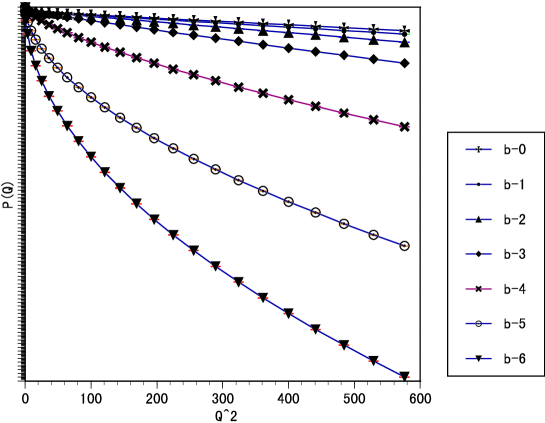
In this subsection we discuss the topological charge distribution $P(Q)$. In Fig. 2, we show the measured $P(Q)$ for various $\beta$’s for a fixed volume $(L=20)$. These $P(Q)$’s have a different behavior between the strong coupling regions and the weak coupling regions. In strong coupling regions, $P(Q)$ exhibits Gaussian behavior. In weak coupling regions, $P(Q)$ deviates gradually from the Gaussian form. In order to investigate the strong coupling regions in detail, we use the chi-square-fitting to $\ln P(Q)$. Table I and II display the results of the fittings, i.e., the coefficients $a_{n}$ of the polynomial $\sum_{n}a_{n}Q^{n}$, for various $\beta$’s with the resulting $\chi^{2}/$ dof, where dof means the degree of freedom. (i)For $\beta\leq 1.5$, the $P(Q)$’s are fitted well by the Gaussian form. (ii)For $2\leq\beta\leq 3$, terms up to the quartic one are needed for sufficiently good fitting. (iii)For $4\leq\beta$, the fittings using the quartic polynomial turn out to be quite poor. Here we discuss the volume dependence. In strong coupling regions, $P(Q)$ is fitted very well by Gaussian form for all values of $V$,

$$P(Q)\propto\exp(-\kappa_{V}(\beta)Q^{2}),$$ (3.1)

where the coefficient $\kappa_{V}(\beta)(=a_{2})$ depends on $\beta$ and $V$. Fig.3 shows $\ln\kappa_{V}(\beta)$ vs. $\ln V$ for a fixed $\beta(=1.0)$. We see that $\kappa_{V}(\beta)$ is clearly proportional to 1/$V$

$$\kappa=\frac{\alpha}{V}$$ (3.2)

This 1/$V$-dependence of the Gaussian behavior determines the phase structure of the strong coupling regions. This result agrees with the $CP^{1}$ result.

Fig. 3: $\ln a_{2}$ vs. $\ln V$ for $\beta=1.0$ and $N=10^{5}$.

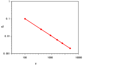
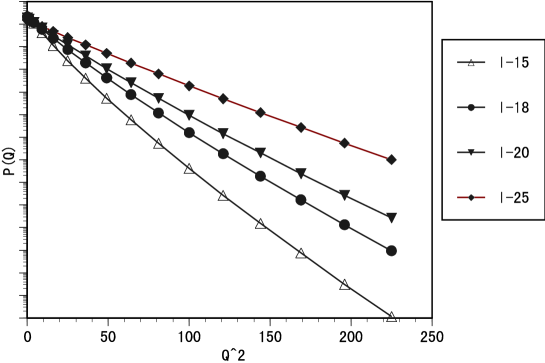
Fig.4 shows the volume dependence of $P(Q)$ for $L=15,18,20,25$ at $\beta=3.45$ . Parameters $a_{1}^{\gamma},\gamma=2.0$ at $\beta=3.45$ (see Table.V) give $V$-dependence. We find slight deviation from exact 1/$V$ law, but a clear volume dependence is observed, which gives $\sim 1/V^{1.15}$, not so far from 1/$V$ law.

Fig. 4: $P(Q)$ vs. $Q^{2}$ for $\beta=3.45$ and $N=5*10^{5}$.

Table I: The results of chi-square-fitting to $\ln P(Q)$ in terms of the polynomial $a_{0}+a_{2}Q^{2}$ for various $\beta$, where dof means degree of freedom.

$\beta$	$\chi^{2}$	$\chi^{2}/$dof	$a_{0}$	$a_{2}$
$0$	$20.058$	$0.872$	$-2.509$	$-0.021$
$1$	$83.936$	$3.649$	$-2.416$	$-0.025$
$1.5$	$136.066$	$5.916$	$-2.368$	$-0.028$
$2$	$769.635$	$34.625$	$-2.296$	$-0.033$

Table II: The result of chi-square-fitting to $\ln P(Q)$ in term of the polynomial $\sum_{n}a_{n}Q^{n}$ for various $\beta$.

$\beta$	$\chi^{2}$	$\chi^{2}/$dof	$a_{0}$	$a_{1}$	$a_{2}$	$a_{3}$	$a_{4}$
$2$	$27.835$	$1.392$	$-2.273$	$0.006$	$-0.035$	$5.123*10^{-5}$	$1.359*10^{-7}$
$3$	$30.561$	$1.528$	$-1.950$	$0.01$	$-0.069$	$5.765*10^{-4}$	$-2.904*10^{-6}$
$4$	$3496.599$	$174.830$	$-0.791$	$-0.684$	$-0.188$	$5.842*10^{-3}$	$-8.643*10^{-5}$
$5$	$4027.247$	$201.362$	$4.147*10^{-3}$	$-4.468$	$-0.159$	$6.161*10^{-3}$	$-1.015*10^{-4}$
$6$	$5175.739$	$258.787$	$-3.341*10^{-3}$	$-8.806$	$-0.054$	$1.423*10^{-3}$	$-1.393*10^{-5}$

3.2 Free energy and expectation value of topological charge

The partition function $Z(\theta)$ is given as a function of $\theta$ by (2.11) from $P(Q)$. The free energy is

$$F(\theta) = -\frac{1}{V}\ln Z(\theta).$$ (3.3)

The expectation value of topological charge is

$$\langle Q\rangle_{\theta} = -(-i)\frac{\displaystyle{dF(\theta})}{\displaystyle{d\theta}}$$ (3.4)

In strong coupling regions, we have Gaussian behavior of $P(Q)$, and the 1/$V$-law appears to hold up to $L=70$. It is natural to expect that this behavior persists to $V\to\infty$. Let us look at how the 1/$V$-law affects $F(\theta)$ and $\langle Q\rangle_{\theta}$. By putting $C(\beta)=9.9$, in $P(Q)=\exp[-\frac{C(\beta)}{V}Q^{2}]$ for $\beta=1.0$, we calculate $F(\theta)$ and $\langle Q\rangle_{\theta}$ from (2.11), (3.3) and (3.4). Figure.5 and 6 show their volume dependence.

Fig. 5: Free energy vs theta in strong coupling regions. $L=4,6,10,20$

Fig. 6: $<Q>$ vs theta in strong coupling regions. $L=4,6,10,20$

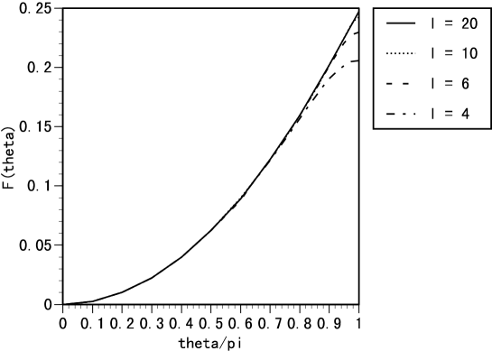
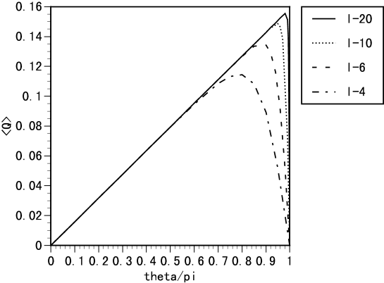
As $V$ is increased, $F(\theta)$ very rapidly approaches a quadratic from in $\theta$ from below. Its first moment $\langle Q\rangle_{\theta}$ develops a peak near $\theta=\pi$, and the position of the peak quickly approaches $\pi$ as $V$ increases. The jump in $\langle Q\rangle_{\theta}$ would arise at $\theta=\pi$ as $V\to\infty$. This indicates the existence of the first order phase transition at $\theta=\pi$.

4 Numerical results II

4.1 Flattening of free energy

Figure 7 shows $F(\theta)$ obtained by “direct method” at $\beta=3.45$.

Fig. 7: Free energy vs theta at $\beta=3.45$ and $L=15,18,20,25$. Flattening is clearly seen in $L=18,20,25$.

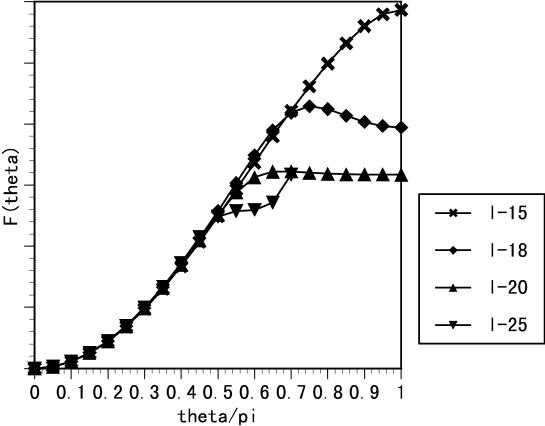
$F(\theta)$ shows “flattening ” at some value $\theta_{f}$ over $L=18$. For $\theta\leq\theta_{f}$, $F(\theta)$ is volume independent. For $\theta_{f}\leq\theta$, $F(\theta)$ is flat. $\theta_{f}$ decreases as $V\to$ large. (In $L=25$, we can not calculate $F(\theta)$ for $\theta\geq 0.7\pi$, because $Z(\theta)$ becomes negative.) This flattening phenomena may correspond to similar behavior found by Schierholz. According to him, such flattening is the position of the first order phase transition ( because $dF/d\theta$ is “discontinuous” at the sharp flattening of free energy $F(\theta)$. Our interpretation about the flattening found in our numerical calculations is different. The shift of $\theta_{f}$ ( flattening position ) with the size of the volume in our calculations is closely related to the statistical error existing in the estimate of $Z(\theta)$ through fourier series. The magnitude of statistical error $\delta P$ in the simulation of $N$ measurements is essentially given by

$$\delta P\sim\frac{1}{\sqrt{N}}.$$ (4.1)

Statistical error $\mathchar 28929\relax P(Q)$ at $Q$ in topological charge distribution $P(Q)$ decreases rapidly with $Q\rightarrow$ large in the set method,

$$\mathchar 28929\relax P(Q)\sim\delta P\times P(Q)$$ (4.2)

where $\delta P=$ constant, and then $\mathchar 28929\relax P(Q)$ is a rapidly decreasing function of $Q$. The largest contribution of $\mathchar 28929\relax P(Q)$ comes from that at $Q=0$,

$$\mathchar 28929\relax P(0)\sim\delta P\times P(0).$$ (4.3)

Then $Z(\theta)$ suffers from the error of $P(0)$ with the magnitude of $\mathchar 28929\relax P(0)\sim\delta P$. The partition function $Z(\theta)$ is also a rapidly decreasing function of $\theta$ and then $Z(\theta)$ becomes the order of $\mathchar 28929\relax P(0)\sim\delta P$ at $\theta\sim\theta_{f}$. In such case, rapidly decreasing function $Z(\theta)$ at $\theta>\theta_{f}$ can not be estimated safely.

We will present the results of our simulation. In table III we show the flattening position $\theta_{f}$ for various lattice sizes $L$ and coupling constants $\beta,\quad\beta=3.45$ and $\beta=3.5$.

Table III: The flattening position $\theta_{f}$ for various lattice sizes $L$. We also show the values of $\theta_{f}\times L$.

$\beta$	$L$	$\theta_{f}$	$\theta_{f}\times L$
3.45	15	0.83$\pi$	$12.4\pi$
	18	$0.7\pi$	$12.6\pi$
	20	$0.6\pi$	$12.1\pi$
	25	$0.51\pi$	$12.8\pi$
3.5	20	$0.57\pi$	$11.4\pi$
	30	$0.38\pi$	$11.4\pi$

From these results, we observe that the flattening position scales as $\theta_{f}\propto L^{-1}=V^{-1/2}$ for each $\beta$, where $V=L^{2}$. What is the reason for this $V^{-1/2}$ -law? At these $\beta$’s, $P(Q)$ is approximately given by gaussian form

$$P(Q)\propto\exp(-\kappa_{V}(\beta)\ \ Q^{2}),$$ (4.4)

and the fourier transform $Z(\theta)$ of this gaussian form is also gaussian form $Z(\theta)=\exp(-\alpha_{V}\theta^{2})$. Then free energy $F(\theta)=-\frac{1}{V}\ln Z(\theta)$ is given by quadratic function $\theta^{2}$. For $L=15$ to $L=25,$ calculated $F(\theta)$ is almost $V$-independent. Since $Z(\theta)=\sum_{Q}P(Q)e^{i\theta Q}$ suffers from the statistical error $\delta P$, flattening is expected at the $\theta$ where the free energy becomes the order of magnitude,

$$VF(\theta_{f})\sim-\ln(\delta P)$$ (4.5)

and we obtain the relation

$$\theta_{f}\sim V^{-1/2}.$$ (4.6)

Of course, $\delta P$ may lead to negative value for $Z(\theta)$ at $\theta\mathrel{\hbox{\raise 0.86108pt\hbox{$>$}\kern-7.5pt\raise-3.87495pt\hbox{$\sim$}}}\theta_{f}$. In $\beta=3.45$, however, $L=15,18,$ and $20$ simulations with $N=5\times 10^{5}$ iterations all give positive $Z(\theta)$ for all $\theta(0\leq\theta\leq\pi)$. Only $L=25$ case leads to negative $Z(\theta)$ at $\theta\mathrel{\hbox{\raise 0.86108pt\hbox{$>$}\kern-7.5pt\raise-3.87495pt\hbox{$\sim$}}}0.7\pi$. We would expect both positive excess fluctuation and negative excess one. So why positive excess results were more often observed in $\beta=3.45$ simulations remains as a question. Numerical results for $Z(\theta)$ and $F(\theta)$ is shown in the table IV for $\beta=3.45$ and $L=20$ case. The value of $Z(\theta)$ in flat region is the same order as $\delta P\sim 1/\sqrt{N}\sim 1.4\times 10^{-3}(N=5\times 10^{5}).$

Table IV: The free energy and partition function for $\beta$=3.45 and $L$=20.

$\theta$	$F(\theta)$	$Z(\theta)$	$\delta Z(\theta)$
$0$	$0$	$1.00$	$1.37*10^{-3}$
$0.1\pi$	$5.65*10^{-4}$	$7.98*10^{-1}$	$1.23*10^{-3}$
$0.2\pi$	$2.23*10^{-3}$	$4.10*10^{-1}$	$9.97*10^{-4}$
$0.3\pi$	$4.92*10^{-3}$	$1.40*10^{-1}$	$9.06*10^{-4}$
$0.4\pi$	$8.48*10^{-3}$	$3.37*10^{-2}$	$8.94*10^{-4}$
$0.5\pi$	$1.26*10^{-2}$	$6.59*10^{-3}$	$8.94*10^{-4}$
$0.6\pi$	$1.56*10^{-2}$	$1.92*10^{-3}$	$8.94*10^{-4}$
$0.7\pi$	$1.61*10^{-2}$	$1.59*10^{-3}$	$9.06*10^{-4}$
$0.8\pi$	$1.59*10^{-2}$	$1.71*10^{-3}$	$9.97*10^{-4}$
$0.9\pi$	$1.59*10^{-2}$	$1.76*10^{-3}$	$1.23*10^{-3}$
$\pi$	$1.59*10^{-2}$	$1.76*10^{-3}$	$1.37*10^{-3}$

Table V: The result of chi-square-fitting to $\ln P(Q)$ in term of the series starting from $a_{0}^{\gamma}+\sum_{n=1}a_{n}^{\gamma}|Q|^{\gamma+n-1}$ for various $\beta$.

$\beta$	$\chi^{2}$	$\chi^{2}/$dof	$\gamma$	$a_{0}^{\gamma}$	$a_{1}^{\gamma}$	$a_{2}^{\gamma}$	$a_{3}^{\gamma}*10^{6}$	$a_{4}^{\gamma}*10^{8}$
$0$	$24.14$	$1.207$	$2.08$	$-2.512$	$-0.0194$	$0.000293$	$-9.32$	$11.8$
$1$	$22.45$	$1.123$	$1.96$	$-2.418$	$-0.0260$	$-0.000155$	$3.73$	$-3.59$
$2$	$29.70$	$1.485$	$2.06$	$-2.267$	$-0.0324$	$0.000383$	$-11.2$	$15.2$
$3.45$	$23.19$	$1.160$	$2.0$	$-1.661$	$-0.122$	$0.00261$	$-39.1$	$1.84$
$4$	$38.98$	$1.949$	$1.59$	$-0.927$	$-0.607$	$0.0104$	$-251$	$287.5$
$5$	$319$	$15.950$	$1.12$	$-0.0274$	$-4.317$	$-0.0157$	$-588$	$684$
$6$	$2813$	$140.65$	$1.09$	$-0.00156$	$-7.534$	$-0.0209$	$268$	$-1210$

Once we found the flattening phenomena in rather large $\beta$ regions, we investigated the strong coupling region again to see whether it is the phenomenon peculiar to weaker coupling regions. Surprisingly, similar phenomenon is found also in strong coupling regions. We show the case of $\beta=1.0$, which is sufficiently strong; chi-square fitting with gaussian form is quite good(Table.I). Fig.1 shown in section 1 is the result obtained for strong coupling region, $\beta=1.0$ and $L=10$ for 500k iterations. Again the position of flattening is consistent with the value estimated from $\delta P$. As is seen above, the calculation of the partition function with the (2.11) using the observed value of $P(Q)$ directly will be called “direct method”. In this method $Z(\theta)$ receives statistical error of the order $\delta P$, and flattening will occur at $\theta_{f}$. On the other hand in the set method, the topological charge distribution itself is obtained over quite wide range of $Q$. We first fit it by appropriate analytical function and using the fitted function $P_{S}(Q)$( “smooth”), we can evaluate $Z(\theta)$. This latter method will be called “fitting method”. In strong coupling regions, the indirect method will lead to gaussian function for $P(Q)$ and the fourier series will again gives gaussian function of $\theta$ for $Z(\theta)$. It gives smooth $\theta^{2}$ type free energy distribution up to $\theta=\pi$. Namely no flattening phenomena will appear.

Actually in $U(1)$ LGT, it is known $P(Q)$ is gaussian for all $\beta$, and $\theta^{2}$ type free energy distribution up to $\theta=\pi$. But if we use the observed $P(Q)$ directly to obtain partition function, it will cause flattening phenomena.

4.2 Strong and weak coupling region

As is seen in Table.I, $\ln P(Q)$ can be fitted by gaussian form well up to $\beta=1.5$, but beyond that value the fitting becomes worse, and higher power terms are necessary. Up to $\beta=3.5$ quartic function fits rather well, still the most dominant power is 2 in this region( see Table.II). In $\beta\geq 4.0$ the power series up to the power 4 is not enough as is seen from Table.II. The value of chi-square become quite bad in $\beta\geq 4.0$. In weaker coupling region ($\beta\mathrel{\hbox{\raise 0.86108pt\hbox{$>$}\kern-7.5pt\raise-3.87495pt\hbox{$\sim$}}}4.0$), we tried another type of function, which is series starting from some power $\gamma$.

$$\ln P(Q)=a_{0}^{\gamma}+\sum_{n=1}a_{n}^{\gamma}|Q|^{\gamma+n-1}$$ (4.7)

This drastically improves the chi-square fit in $4.0\mathrel{\hbox{\raise 0.86108pt\hbox{$>$}\kern-7.5pt\raise-3.87495pt\hbox{$\sim$}}}\beta\mathrel{\hbox{\raise 0.86108pt\hbox{$>$}\kern-7.5pt\raise-3.87495pt\hbox{$\sim$}}}5.0$ (see Table.V. and compare with Table.II.). The chi-square value for $\beta=4$ was 3497 in Table.II, it becomes 38.98 in Table.V. From Table.V, we understand that leading power $\gamma$ is 2 for $\beta\mathrel{\hbox{\raise 0.86108pt\hbox{$<$}\kern-7.5pt\raise-3.87495pt\hbox{$\sim$}}}3.5$ and the leading power becomes 1 in $\beta\mathrel{\hbox{\raise 0.86108pt\hbox{$>$}\kern-7.5pt\raise-3.87495pt\hbox{$\sim$}}}5$, thus we will call this region weak coupling region. $\beta=4.0$ is “intermediate”, since leading power $\gamma$ is about 1.59, which is just medium value of $\gamma=$2(gaussian in strong coupling regions) and $\gamma$=1(weak coupling regions).

In weak coupling regions excitation of topological charge is suppressed stronger as $\beta$ becomes larger. For example,

$$\frac{P(2)}{P(1)}=\frac{1}{1.12},\quad\frac{1}{3.3},\quad\frac{1}{126}$$ (4.8)

for $\beta=2.0,4.0,5.0$ respectively.

On the contrary large topological charge configuration is relatively important and gaussian distribution is obtained in strong coupling region. It leads to the partition function, $\vartheta_{3}(\nu,\tau)$, third elliptic theta function. Here $\nu=\theta/({2\pi}),\tau=i\kappa_{V}(\beta)/\pi$. Note that $\theta$ is extended to complex values. This function clearly shows the distribution of partition function zeros leading to the first order phase transition at $\theta=\pi$.

In weak coupling regions large topological charge contribution is suppressed. In this region $-\ln P(Q)$ is given approximately by $a^{\gamma}_{1}|Q|$( with $\gamma\sim 1.0$). This form of $P(Q)$ leads to the partition function given by the generating function of Chebyshev Polynomials.

$$Z(\theta) = \sum^{\infty}_{Q=-\infty}c^{|Q|}e^{i\theta Q}$$ (4.9)

$$= \frac{1-c^{2}}{1-2c\cos\theta+c^{2}}$$ (4.10)

In weak coupling regions, the value of $c$ is quite small and $c^{2}$ in this equation can be discarded. It leads to the expectation value of topological charge almost given by $\sin\theta$ form.

$$i<Q>=\frac{1}{V}\frac{dZ}{d\theta}/Z\sim\frac{2c}{V}\sin\theta$$ (4.11)

when $|c|<<1$. At $\beta=6.0,L=20$, the value of $c$ is $c=1.34\times 10^{-4},2c/V\sim 6.68\times 10^{-7}$. Actually calculated $i<Q>$ shows sine function type behavior over whole range of $\theta$ in weak coupling regions. No discrete phase transition is expected at $\theta=\pi$ in weak coupling regions. Whether there is a continuous phase transition( second order one) or not needs further precise investigation such as study of correlation length.

5 Conclusoins and discussion

In this paper we have investigated two dimensional $CP^{2}$ model with $\theta$-term numerically. Topological charge distribution is measured by Monte Carlo method based on set method and trial function method. Then it is used to obtain partition function $Z(\theta)$ as a function of theta parameter.

Topological charge distribution $P(Q)$ is gaussian in strong coupling regions( $\beta\mathrel{\hbox{\raise 0.86108pt\hbox{$<$}\kern-7.5pt\raise-3.87495pt\hbox{$\sim$}}}1.5$). In $\beta=2\sim 3.5$ region, the exponent of $P(Q)$ can not be simply given by $Q^{2}$ but additional higher powers are necessary(Table I and II). Still the leading contribution comes from $Q^{2}$ term(Table V).

In weak coupling regions, i.e., $\beta\mathrel{\hbox{\raise 0.86108pt\hbox{$>$}\kern-7.5pt\raise-3.87495pt\hbox{$\sim$}}}4.5$, the leading power of exponent of $P(Q)$ is $|Q|$. Sharp decrease of $P(Q)$ at larger $|Q|$ is observed.

At $\beta=4$, which is intermediate of strong and weak coupling region is characterized by leading power of exponent of $P(Q)$ is given by $|Q|^{1.59}$, whose exponent is the intermediate value of $Q^{2}$( gaussian $P(Q)$ ) in strong coupling region and $|Q|^{1}$ in weak coupling region.

Free energy as a function of $\theta$ is investigated. We observed “flattening ” of $\theta$-distribution of free energy at $\theta_{f}$. In our analysis, the main reason of this flattening is attributed to the statistical fluctuation $\delta P$ of $P(Q)$ at $Q=0$ and $\delta P\sim O(1/\sqrt{N})$, where $N$ is the number of measurements. Volume dependence at each $\beta$ is explained by this interpretation.

Topological charge distribution $P(Q)$ is measured over wide range of $Q$. But direct method to obtain $Z(\theta)$ through fourier series with direct use of measured topological charge distribution $P(Q)$ leads to flattening caused by $\delta P$. We tried to obtain approximate form of $P(Q)$ by fitting method. The smooth function $P(Q)_{S}$ obtained by fitting and used to evaluate $Z(\theta)_{S}$ has following properties. In strong coupling region, the gaussian topological charge distribution leads to $Z(\theta)_{S}$ with the third elliptic theta function $\vartheta_{3}$ and it leads to infinite number of zeros of partition function leading to the first order phase transition at $\theta=\pi$ in infinite volume limit. In weak coupling region, $Z(\theta)_{S}$ is approximated by the functional form

$$Z(\theta)_{S}=\frac{1-c^{2}}{1-2\cos\theta+c^{2}},\quad(c<<1)$$ (5.1)

which is the generating function of Chebyshev polynomials. Due to this form, the expectation value of topological charge

$$i<Q>\propto\sin\theta$$ (5.2)

No first order phase transition at $\theta=\pi$ is expected.

A Integration Measure

In this appendix, we will discuss briefly about the measure of integration. The measure is defined as

$$dz_{1}dz_{2}dz_{3}\delta(|z_{1}|^{2}+|z_{2}|^{2}+|z_{3}|^{2}-1).$$ (A.1)

The complex numbers $z_{i}(i=1,2,3)$ are given by two real numbers $x_{i},y_{i}$ as $z_{i}=x_{i}+iy_{i}$. The measure becomes

$$dx_{1}dy_{1}dx_{2}dy_{2}dz_{3}dz_{3}\delta(x_{1}^{2}+y_{2}^{2}+x_{2}^{2}+y_{2}^{2}+x_{3}^{2}+y_{3}^{2}-1).$$ (A.2)

When the parameters $x_{i},y_{i}(i=1,2,3)$ are changed to polar coordinates $(k_{i},a_{i}(i=1,2,3))$

$$x_{i} = k_{i}\cos a_{i},$$ (A.3)

$$y_{i} = k_{i}\sin a_{i},$$ (A.4)

where $k_{i}\geq 0$ and $0\leq a_{i}\leq 2\pi$. The measure becomes

$$k_{1}\ k_{2}\ k_{3}\ dk_{1}\ dk_{2}\ dk_{3}\ \delta(k_{1}^{2}+k_{2}^{2}+k_{3}^{2}-1)\ da_{1}\ da_{2}\ da_{3}.$$ (A.5)

We translate the parameters from $k_{1},k_{2},k_{3}$ to 3 dimensional polar coordinates $(l,t_{1},t_{2})$

$$k_{1} = l\sin t_{1}\cos t_{2},$$ (A.6)

$$k_{2} = l\sin t_{1}\sin t_{2},$$ (A.7)

$$k_{3} = l\cos t_{2},$$ (A.8)

$$l^{5}\ \delta(l^{2}-1)\sin^{3}t_{1}\cos t_{1}dt_{1}\sin t_{2}\cos t_{2}\ dl\ da_{1}\ da_{2}\ da_{3},$$ (A.9)

where $l\geq 0$ and $0\leq t_{1},t_{2}\leq\frac{\pi}{2}$. So the measure which we use in Monte Carlo simulation becomes finally

$$dm\ dn\ da_{1}\ da_{2}\ da_{3},$$ (A.10)

after integration about $l$ is done. The variables $m,n$ are given by

$$m = \frac{1}{8}(\cos 2t_{2}-\frac{1}{4}\cos 4t_{1}),$$ (A.11)

$$n = \frac{1}{4}\cos 2t_{2}.$$ (A.12)

References

- [1] K. G. Wilson, Phys. Rev. D10 (1974), 2445.
- [2] M. Creutz, Phys. Rev. D21 (1980), 2308.
- [3] G. Bhanot, S. Black, P. Carter and R. Salvador, Phys. Lett. B183 (1987), 331.
- [4] G. Bhanot, R. Dashen, N. Seiberg and H. Levine, Phys. Rev. Lett. 53 (1984), 519.
- [5] U. -J. Wiese, Nucl. Phys. B318 (1989), 153.
- [6] M. Karliner, S. Sharpe and Y. F. Chang, Nucl. Phys. B302 (1988), 204.
- [7] W. Bietenholz, A. Pochinsky and U. -J. Wiese, Phys. Rev. Lett. 75 (1995), 4524
- [8] B. Berg and M. Lüscher, Nucl. Phys. B190[FS3] (1981), 412.
- [9] S. Olejnik and G. Schierholz, Nucl. Phys. B(Proc. Suppl)34,(1994),709; G. Schierholz, Nucl. Phys. B(Proc. Suppl)37A,(1994),203.
- [10] J. C. Plefka and S. Samuel, Phys. Rev. D56 (1997), 44.
- [11] S. Coleman, Ann. of Phys. 101 (1976), 239.
- [12] A.S. Hassan,M. Imachi,N. Tsuzuki and H. Yoneyama, Prog. Theor. Phys 94 (1995), 861.
- [13] J. L. Cardy and E. Rabinovici, Nucl. Phys. 205[FS5] (1982), 1 ;J. L. Cardy, Nucl. Phys. 205[FS5] (1982), 17.
- [14] G. ,t Hooft, Nucl. Phys. 190[FS3] (1981), 455.
- [15] A.S. Hassan,M. Imachi,N. Tsuzuki and H. Yoneyama, Prog. Theor. Phys 95 (1996), 175.
- [16] M. E. Fisher and A. N. Berker,Phys. Rev. B26 (1982), 2507.
- [17] C. Itzykson, R. B. Perason and J. B. Zuber, Nucl. Phys. B220[FS8] (1983), 415.
- [18] N. Seiberg, Phys. Rev. Lett. 53 (1984), 637.
- [19] M. Imachi, S. Kanou and H. Yoneyama, hep-lat/9809139(1998).