Multi-histogram Reweighting for Finite Density Lattice QCD

Abstract:

Finite density simulations require dynamical fermions which are computationally demanding. We employ Ferrenberg and Swendsen reweighting method to reduce the number of ensembles needed. We use their method to do a combined reweighting in both $\beta$ and quark number $k$ on an ensemble generated by the Kentucky group.

1 Introduction

Finite density simulations require dynamical fermions which are computationally demanding. When studying phase transitions we have to scan very finely both the temperature and density directions; a large number of ensembles need to be generated. Ferrenberg and Swendsen [1] [2] showed that we can employ reweighting to reduce the number of ensembles needed. Using their methods we perform an extrapolation in $\beta$ and then we do a combined reweighting in both $\beta$ and the quark number $k$. We take the ensembles generated at $k=0$ and $k=3$, and used them to extrapolate to $k=6$ case. The results of reweighting are also compared against the ones of that direct measurements.

2 Simulation Background

Finite density ensembles were generated using the canonical approach [3]. To build canonical partition function,we start from fugacity expansion of the grand canonical partition function,

$$Z(V,T,\mu)=\sum_{k}Z_{C}(V,T,k)e^{\mu k/T},$$ (1)

where $k$ is the net quark number, $Z_{C}$ is the canonical partition function of the system. On a lattice, we can easily compute the Fourier transform of the grand canonical partition function

$$Z(V,T,\mu)=\int\mathop{{\cal D}\hbox{U}}\mathop{{\cal D}\bar{\psi}{\cal D}\psi}e^{-S_{g}(U)-S_{f}(\mu;U,\bar{\psi},\psi)}$$ (2)

to get the canonical partition function

$$Z_{C}(V,T,k)=\frac{1}{2\pi}\int_{0}^{2\pi}\mbox{d}\phi\,e^{-ik\phi}Z(V,T,\mu)|_{\mu=i\phi T}.$$ (3)

We will specialize to the case of two degenerate flavors. After integrating out the fermion part, we get a simple expression

$$Z_{C}(V,T,k)=\int\mathop{{\cal D}\hbox{U}}e^{-S_{g}(U)}\mbox{det}_{k}M^{2}(U),$$ (4)

where

$$\mbox{det}_{k}M^{2}(U)\equiv\frac{1}{2\pi}\int_{0}^{2\pi}\mbox{d}\phi\,e^{-ik\phi}\det M(m,\mu;U)^{2}|_{\mu=i\phi T}$$ (5)

is the determinant projection to the fixed net quark number $k$. Then $Z_{C}$ is used to generate the ensembles at particular $k$.

Simulations based on the action give in (4) cannot be carried out directly since the integrand is not positive definite. The determinant is split in two parts: a positive definite part that is used to generate the ensemble and a phase. For a more detailed presentation we refer the reader to the original paper [3].

The absolute value of the Polyakov loop is given by

$$\left<|P|\right>=\frac{\left<|P|\alpha\right>_{0}}{\left<\alpha\right>_{0}},$$ (6)

where

$$\alpha(U)=\frac{\widetilde{\mbox{det}}_{k}M^{2}(U)}{\left|\mathop{\hbox{Re}}\widetilde{\mbox{det}}_{k}M^{2}(U)\right|},~{}~{}\widetilde{\mbox{det}}_{k}M^{2}(U)\equiv\frac{1}{N}\sum_{j=0}^{N-1}e^{-ik\phi_{j}}\det M(U_{\phi_{j}})^{2}$$ (7)

is the phase and $\left<\right>_{o}$ stands for the average over the ensemble generated with measure $\left|\mathop{\hbox{Re}}\widetilde{\mbox{det}}_{k}M^{2}(U)\right|$. Quark chemical potential is defined by the expression below:

$$\mu(k) = -\frac{1}{\beta}\ln\frac{\tilde{Z}_{C}(k+1)}{\tilde{Z}_{C}(k)}=-\frac{1}{\beta}\ln\frac{1}{\tilde{Z}_{C}(k)}\int\mathop{{\cal D}\hbox{U}}e^{-S_{g}(U)}$$ (8)

$$\times \frac{1}{N}\sum_{j=0}^{N-1}e^{-i\phi_{j}}e^{-ik\phi_{j}}\det M^{2}(U_{\phi_{j}})$$

$$= -\frac{1}{\beta}\ln\left<e^{-i\phi}\right>_{k}.$$

More relevant to our study is the baryon chemical potential:

$$\mu_{B}(n_{B})=-\frac{1}{\beta}\ln\left<e^{-i3\phi}\right>_{3n_{B}}.$$ (9)

To test the reweighting method, a subset of the original ensembles was employed and the results of the extrapolation were compared against the results of the direct measurements.

3 Algorithm

The original reweighting method [1] employed an ensemble generated at a particular point in the parameter space to build an “induced” ensemble for a different value of parameters. The method is limited to a neighborhood of the original point in the parameter space. At distant points the extrapolation becomes unreliable due to poor overlap between the original and the target distribution.

The multi-histogram method [2] addresses the limitations of the original method by employing several ensembles. A carefully chosen set of ensembles, covering the area of interest in the parameter space, allows us to interpolate reliably. Thus, we can finely scan the area of interest with only a small set of ensembles.

The basic idea behind the reweighting method is to use the histogram generated by the simulated ensembles as an approximation of the probability distribution; this approximation is then used to approximate the probability distribution at a different point in the parameter space. Once we have an approximation for the probability distribution we can compute all observables.

We used these methods in two scenarios:

1. Fix $k$, vary $\beta$.

   • Single histogram method: The histogram of only one ensemble is used in this case.

   • Multi-histogram method: The histograms of several ensembles generated at different points are combined.

2. Vary both $\beta$ and $k$. (Only Multi-histogram method is used.)

In our first case (fix $k$, vary $\beta$), we approximate the “weight” of each configuration $U$ by

$$P(U,\beta)=\frac{e^{-S_{\beta}(U)}}{\sum_{m=1}^{R}n_{m}e^{-S_{\beta_{m}}(U)-f_{m}}}$$ (10)

This approximation allows us to compute averages at arbitrary values of $\beta$. The input for this formula consists of $R$ ensembles generated by weights given by $S_{\beta_{1}},\ldots,S_{\beta_{R}}$ with $n_{1},\ldots,n_{R}$ configurations in each ensemble.

To use the formula above we need to determine the parameters $f_{n}$ — they are the “free energies” of each ensemble $n$,

$$exp(f_{n})=\sum_{U_{i}}P(U_{i},\beta_{n})$$ (11)

where we sum over all the configurations $U_{i}$ in the ensemble. Eq. (10) and  (11) are used to determine the free energy $f_{n}$. We start with a guess for $f_{n}$ and plug this into Eq. (10) to get an approximation for the probability distribution $P(U,\beta)$. Then, we take this approximation for $P(U,\beta)$ and plug it into Eq. (11) to get a more refined guess of $f_{n}$. We repeat this process until $f_{n}$ converges.

After convergence is reached, we can measure the observables at different $\beta$ by

$$<O>_{\beta}=\frac{\sum_{U}O(U)P(U,\beta)}{\sum_{U}P(U,\beta)}$$ (12)

For our second case (both $\beta$ and $k$ are varied), the “weight” for different configurations at different $k$ and $\beta$ should be calculated as

$$P(U,k^{\prime},\beta^{\prime})=\frac{|\mathop{\hbox{Re}}\mbox{det}_{k^{\prime}}M^{2}(U)|e^{-S_{\beta^{\prime}}(U)}}{\sum_{i=1}^{R}n_{i}|\mathop{\hbox{\hbox{Re}}}\mbox{det}_{k_{i}}M^{2}(U)|e^{-S_{\beta_{i}}(U)-f_{i}}}$$ (13)

$$\exp(-f_{i})=\sum_{U_{j}}P(U_{j},k_{i},\beta_{i})~{}~{}~{}\mbox{\small We sum over all configurations}$$ (14)

The chemical potential can be measured by using the “weight” $P(U,k,\beta)$:

$$\beta\mu_{B}(n_{B},\beta) = -\mbox{ln}\frac{1}{Z_{c}(3n_{B},\beta)}\int{\cal D}Ue^{-S_{\beta}(U)}$$ (15)

$$\times\frac{1}{N}\sum_{j=0}^{N-1}e^{-i3\phi_{j}}e^{-i3n_{B}\phi_{j}}\mbox{det}M^{2}(U_{\phi_{j}})$$

Optimized convergence

In our calculations, we found that the iteration presented above converges very slowly. For a more efficient convergence we use the following procedure: we know that $\vec{f}^{(k+1)}$ (the $k+1^{th}$ iteration step) can be expressed as a function of $\vec{f}^{(k)}$ ($k^{th}$ step)

$$\vec{f}^{(k+1)}=\vec{G}(\vec{f}^{(k)})~{}~{}~{}\vec{G}~{}\mbox{is the vector function of}~{}\vec{f}^{(k)}$$ (16)

In our case, $\vec{f}$ is the free energy, $\vec{G}$ is the recurrent equation (14) for the free energy calculation. The fixed point $\vec{f}^{(\infty)}$ has the property that $\vec{f}^{(\infty)}=\vec{G}(\vec{f}^{(\infty)})$. At step $k$ our approximation is $\vec{f}^{(k)}$, we write then:

$$\vec{f}^{(k)}+\delta{\vec{f}^{(k)}}=\vec{G}(\vec{f}^{(k)}+\delta{\vec{f}^{(k)}})~{}~{}~{}\mbox{where}~{}~{}~{}\delta{\vec{f}^{(k)}}=\vec{f}^{(\infty)}-\vec{f}^{(k)}.$$ (17)

Assuming that $\vec{f}^{(k)}$ is close to $\vec{f}^{(\infty)}$ then $\delta{\vec{f}^{(k)}}$ is small and we can approximate

$$\vec{G}(\vec{f}^{(k)}+\delta{\vec{f}^{(k)}})\approx\vec{G}(\vec{f}^{(k)})+\triangledown\vec{G}\cdot\delta{\vec{f}^{(k)}}.$$ (18)

Using this we get:

$$f_{i}^{(k)}+\delta{f_{i}^{(k)}}\approx G_{i}(\vec{f}^{(k)})+\frac{\partial{G_{i}}}{\partial{f_{j}^{(k)}}}\delta{f_{j}^{(k)}}$$ (19)

$\frac{\partial{G_{i}}}{\partial{f_{j}^{(k)}}}$ is the element of matrix $M^{(k)}=\frac{\partial{G_{i}}}{\partial{f_{j}^{(k)}}}$,

$$f_{i}^{(k)}+\delta{f_{i}^{(k)}}\approx G_{i}(\vec{f}^{(k)})+M_{ij}^{(k)}\delta{f_{j}^{(k)}}$$ (20)

so

$$(I-M^{(k)})_{ij}\delta{f_{j}^{(k)}}\approx G_{i}(\vec{f}^{(k)})-f_{i}^{(k)}$$ (21)

$$\delta{f_{j}^{(k)}}\approx(G_{i}(\vec{f}^{(k)})-f_{i}^{(k)})\cdot{(I-M^{(k)})^{-1}}_{ij}$$ (22)

We expect the matrix $(I-M^{(k)})$ to be almost singular when we are approaching fixed point, so we use SVD to compute the matrix inversion. Our next step in the iteration is then $\vec{f}^{(k+1)}=\vec{f}^{(k)}+\delta\vec{f}^{(k)}$ rather than $\vec{G}(\vec{f}^{(k)})$. Using this method the convergence of the iteration is greatly accelerated.

4 Results and Conclusion

We determine the Polyakov loop using the single histogram method and the multi-histogram method and compare the results with the direct measurements. The results are plotted as a function of $\beta$, the gauge coupling constant.

Figure 1: Polyakov loop (Single histogram at fixed $k=3$). All dots represent the ensembles where direct measurements were carried out. The ones surrounded with polygon are used as our reweighting input; the gray ones are not. The line represents the result of the extrapolation and the band represents the statistical errors.

From single histogram reweighting of Polyakov loop, we can see from Fig. 1 the method is limited to a neighborhood of the original point $\beta=5.20$ in the parameter space. The extrapolation at distant points becomes unreliable due to poor overlap. The multi-histogram method addresses this limitation, and by employing several ensembles, we expect to interpolate results reliably.

a	b
c	d

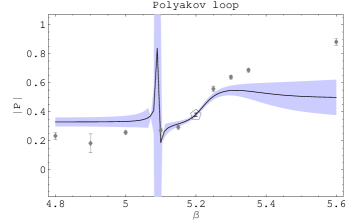
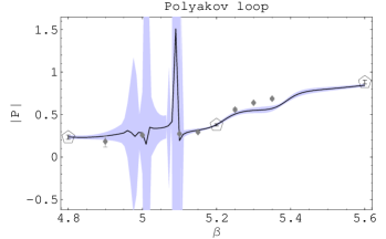
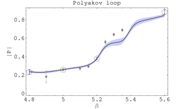
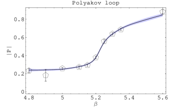
Figure 2: Polyakov loop(Multi-histogram, fixed $k=3$). Same as in Fig. 1 for multi-histogram reweighting with k=3. From a to b, more ensembles are added.

We start by employing three ensembles in Fig. 2. Two of them at $\beta=4.8$ and $\beta=5.6$ are the bounds of the region of interest and the third one is in the middle at $\beta=5.2$. We plot the results in Fig. 2a; we see that the error bars are quite large between $\beta=4.9$ and $5.1$. When we add one more ensemble in the “problem” region, the plot changes significantly as we can see from Fig. 2b. The largest error bars are around $\beta=5.3-5.4$ now. Once we add a point at $\beta=5.3$ the error bars are reduced as we see from Fig. 2c. From this plot we also see that with only half of the generated ensembles the reweighting curve describes very well the data in the region of interest. From Fig. 2d, we see that adding more ensembles (total 10 ensembles) doesn’t change the curve significantly — the only difference is that the error band gets smaller.

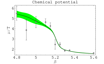
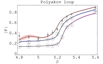
Figure 3: We used ensembles generated at $k=0$ and $k=3$ to extrapolate $k=6$ case, and the plot is compared to the direct measurements.

We have also performed a combined reweighting in $\beta$ and $k$ in Fig. 3. We employed ten ensembles at $k=0$ and ten ensembles at $k=3$ to extrapolate to $k=6$. We used this method to compute both the Polyakov loop and the chemical potential. As we can see from Fig. 3 the extrapolated curve matches rather well the direct measurements.

We find that multi-histogram method can be used effectively to reduce the number of ensembles needed for our simulations: for our $\beta$ interpolations we find that we could use as little as half of the ensembles generated to get a much better scan of the temperature range. The way we envision using this method is to generate few ensembles of first scanning the temperature range rather coarsely and then add some more ensembles at the points where “features” like sharp transitions appear in our plots. The process stops when adding new ensembles does not alter our plots significantly. We also find that interpolations in both temperature and quark number are feasible and we plan to employ these methods in our further studies.

References

• [1] A. M. Ferrenberg and R. H. Swendsen, Phys. Rev. Lett. 61, 2635 (1988)
• [2] A. M. Ferrenberg and R. H. Swendsen, Phys. Rev. Lett. 63, 1195 (1989)
• [3] A. Alexandru, M. Faber, I. Horv th, K. Liu, Phys. Rev. D72, 114513 (2005)