Testing and tuning symplectic integrators for Hybrid Monte Carlo algorithm in lattice QCD

Abstract

We examine a new 2nd order integrator recently found by Omelyan et al. The integration error of the new integrator measured in the root mean square of the energy difference, $\langle\Delta H^{2}\rangle^{1/2}$, is about 10 times smaller than that of the standard 2nd order leapfrog (2LF) integrator. As a result, the step size of the new integrator can be made about three times larger. Taking into account a factor 2 increase in cost, the new integrator is about 50% more efficient than the 2LF integrator. Integrating over positions first, then momenta, is slightly more advantageous than the reverse. Further parameter tuning is possible. We find that the optimal parameter for the new integrator is slightly different from the value obtained by Omelyan et al., and depends on the simulation parameters. This integrator could also be advantageous for the Trotter-Suzuki decomposition in Quantum Monte Carlo.

1 Introduction

The Hybrid Monte Carlo (HMC) algorithm[1] is now the established standard for the generation of dynamical fermion configurations in lattice Quantum Chromo Dynamics (QCD). The HMC algorithm consists of molecular dynamics (MD) trajectories, each followed by a Metropolis test. During the MD trajectory, one integrates Hamilton’s equations of motion, using an integrator with a discrete stepsize $\Delta t$ which must satisfy two conditions in order to maintain detailed balance: $(i)$ simplecticity (the phase space volume $dpdq$ must be conserved) and $(ii)$ time reversibility. The simplest and most widely used integrator wih these properties is the 2nd order leap frog (2LF) integrator, which causes ${\cal O}(\Delta t^{2})$ errors in the total energy or Hamiltonian. These errors are eliminated at the Metropolis accept/reject step, which makes the algorithm exact.

The acceptance at the Metropolis step depends on the magnitude of the error in the total energy. In order to reduce the error and thus increase the acceptance one could use higher order integrators. Early attempts, however, did not appear to be practical [2, 3]. This is because the efficiency of higher order integrators depends largely on the system size and these early attempts were made on rather small lattices. As the lattice size increases above a certain value $V_{c}$, the higher order integrators should perform better than the low order integrator. This minimum lattice size $V_{c}$ depends on the Hamiltonian which we consider and on the choice of integrator. For lattice QCD, it turned out that $V_{c}$ becomes very large at small quark masses, so that on currently accessible computers the 2LF integrator is the best choice[4] for simulations at zero temperature. At finite temperature, higher order integrators could perform better on moderate-size lattices[5]: this is because chiral symmetry gets restored, so that small Dirac eigenvalues disappear, which allows for stable MD integration using larger stepsizes.

So far, only the 2LF integrator has been considered in the HMC algorithm of lattice QCD as a second order integrator, because of its simplicity and effectiveness. Recently however, Omelyan et al. [6] found a new 2nd order integrator which is expected to be better than the 2LF integrator although it has twice the computational cost. Here we examine this new 2nd order integrator for the HMC algorithm in lattice QCD and measure its efficiency. We also examine the new 4th order integrators recommended in [6]. Finally, we try to further tune the new 2nd order integrator.

2 Symplectic Integrator

2.1 Recursive construction scheme

Symplectic integrators are most conveniently described by the Lie algebra formalism[7, 8, 9]. Let $H$ be a classical Hamiltonian,

$$H=\frac{1}{2}p^{2}+S(q),$$ (1)

where $q=(q_{1},q_{2},\dots)$ and $p=(p_{1},p_{2},\dots)$ are coordinate variables and conjugate momenta respectively. Hamilton’s equations are expressed as

$$\dot{f}=\{f,H\},$$ (2)

where $f=q$ or $p$ and $\{,\}$ stands for the Poisson bracket,

$$\{f,H\}=\sum_{i}\left(\frac{\partial f}{\partial q_{i}}\frac{\partial H}{\partial p_{i}}-\frac{\partial f}{\partial p_{i}}\frac{\partial H}{\partial q_{i}}\right).$$ (3)

If we define the linear operator $L(H)$ as

$$L(H)f\equiv\{f,H\},$$ (4)

then we can write the formal solution of Hamilton’s equations,

$$f(t+\Delta t)=\exp(\Delta tL(H))f(t).$$ (5)

In general the operator $\exp(\Delta tL(H))$ cannot be expressed exactly in a simple form. Therefore we approximate $\exp(\Delta tL(H))$ with an operator correct up to a certain order in $\Delta t$. Let us write $L(H)$ as

$$L(H) = L(\frac{1}{2}p^{2})+L(S(q)),$$ (6)

$$= T+V,$$ (7)

where $T\equiv L(\frac{1}{2}p^{2})$ and $V\equiv L(S(q))$. The 2LF integrator is given by decomposing $e^{\Delta t(T+V)}$ as

$$\exp(\Delta t~{}(T+V))=\exp(\frac{1}{2}\Delta t~{}T)\exp(\Delta t~{}V)\exp(\frac{1}{2}\Delta t~{}T)+{\cal O}(\Delta t^{3}).$$ (8)

We call $G_{2}(\Delta t)$ the 2LF integrator:

$$G_{2}(\Delta t)\equiv\exp(\frac{1}{2}\Delta t~{}T)\exp(\Delta t~{}V)\exp(\frac{1}{2}\Delta t~{}T).$$ (9)

The integrator $G_{2}(\Delta t)$ amounts to mapping $q$ and $p$ to new variables as

$$\left(\begin{array}[]{c}q(t+\Delta t)\\ p(t+\Delta t)\end{array}\right) = \left(\begin{array}[]{cc}1&\frac{1}{2}\Delta t\\ 0&1\end{array}\right)\bullet\left(\begin{array}[]{cc}1&0\\ -\frac{\partial S(q)}{\partial q}\frac{\Delta t}{q}&1\end{array}\right)\bullet\left(\begin{array}[]{cc}1&\frac{1}{2}\Delta t\\ 0&1\end{array}\right)\bullet\left(\begin{array}[]{c}q(t)\\ p(t)\end{array}\right)$$ (20)

$$\equiv G_{2}(\Delta t)\bullet\left(\begin{array}[]{c}q(t)\\ p(t)\end{array}\right).$$ (23)

This map is symplectic. This is easy to see, since the three matrices representing the elementary substeps are triangular with determinant 1. It is also exactly time-reversible: $G_{2}(\Delta t)G_{2}(-\Delta t)=1$.

An equivalent algorithm is obtained by interchanging $T$ and $V$ in eq.(9).

Higher order integrators can also be found by decomposing $e^{\Delta t(T+V)}$ to the desired order. Although the decomposition to a higher order is a non-trivial problem with no unique solution, there is a simple recursive construction scheme which generates higher order integrators from lower order ones[3, 10, 8]. In this scheme, the $(2k+2)$-th order integrator is given by

$$G_{2k+2}(\Delta t)=G_{2k}(b_{1}\Delta t)G_{2k}(b_{2}\Delta t)G_{2k}(b_{1}\Delta t),$$ (24)

where

$$b_{1}=\frac{1}{2-2^{1/(2k+1)}},$$ (25)

$$b_{2}=1-2b_{1}=-\frac{2^{1/(2k+1)}}{2-2^{1/(2k+1)}}.$$ (26)

Let us call the integrators of eq.(24) recursive construction (RC) integrators. These integrators are symplectic and constructed in a symmetric way, thus time reversible, i.e. $G_{2k+2}(\Delta t)G_{2k+2}(-\Delta t)=1$. Note that $b_{2}$ is negative. The appearance of negative coefficients in higher order integrators is inevitable: beyond the 2nd order decomposition there is no decomposition scheme having positive coefficients only[11]. However if we include the commutator $[V,[T,V]]$ in the decomposition we may circumvent this situation[12, 13], and integrators with all positive coefficients can be constructed. Even so, the inclusion of this commutator requires the calculation of the gradient of the force, which increases the computational cost. If the force-gradient calculations are computationally simple for the system considered, then it would be worth considering such integrators. For lattice QCD, it is unclear that such force-gradient integrators have advantages over the non-force-gradient ones. We do not consider such force-gradient integrators here.

2.2 Minimum norm construction scheme

Although the recursive construction scheme makes it easy to construct higher order integrators to any order, their performance may not be optimal, since the number of force calculations grows rapidly with the order of the integrator. More generally, one can decompose $e^{\Delta t(T+V)}$ as

$$\exp(\Delta t~{}(T+V))=\Pi_{i}^{k}\exp(c_{i}\Delta t~{}T)\exp(d_{i}\Delta t~{}V)+{\cal O}(\Delta t^{n+1}),$$ (27)

where $\sum_{i}^{k}c_{i}=\sum_{i}^{k}d_{i}=1$. Moreover, in order to form a time-reversible integrator certain relations must be hold. For instance if we take $k=3$, the following equations must be satisfied: $(i)$$c_{1}=c_{4},c_{2}=c_{3},d_{1}=d_{3},d_{4}=0$ or $(ii)$$c_{1}=0,c_{2}=c_{4},d_{1}=d_{4},d_{2}=d_{3}$. For time-reversible integrators, the error terms with odd $n$ always vanish[3, 8, 11]. Thus time-reversible integrators have a leading error term ${\cal O}(\Delta t^{n+1})$ with $n$ even.

The error term ${\cal O}(\Delta t^{n+1})$ consists of commutators of $T$ and $V$. For instance, the leading error terms of the 2nd and 4th order integrators are respectively [6]

$${\cal O}(\Delta t^{3})=\alpha[T,[V,T]]+\beta[V,[V,T]],$$ (28)

and

$${\cal O}(\Delta t^{5})=\gamma_{1}[T,[T,[T,[T,V]]]]+\gamma_{2}[T,[T,[V,[T,V]]]]+\gamma_{3}[V,[T,[T,[T,V]]]]+\gamma_{4}[V,[V,[T,[T,V]]]],$$ (29)

where $\alpha$, $\beta$ and $\gamma_{i}$ depend on $c_{i}$ and $d_{i}$.

One strategy to find optimal integrators in the absence of further information about the operators $T$ and $V$ is to minimize the norm of the error coefficients. For the case of eq.(28) and (29), this strategy implies minimizing the following error functions:

$$Err_{3}\equiv\sqrt{\alpha^{2}+\beta^{2}},$$ (30)

and

$$Err_{5}\equiv\sqrt{\gamma_{1}^{2}+\gamma_{2}^{2}+\gamma_{3}^{2}+\gamma_{4}^{2}}.$$ (31)

Omelyan et al. [6] found a class of integrators by following this strategy. Among the new integrators which they identified, they found several “outstanding” integrators having especially small norms of the error coefficients. In this analysis, we consider the new 2nd and 4th order integrators which they recommend as outstanding integrators, and which are described as follows.

2.2.1 2nd order minimum norm (2MN) integrator

Omelyan et al. [6, 15] obtained the following new 2nd order integrator.

$$I_{2MN}(\Delta t)=e^{\lambda\Delta tT}e^{\frac{\Delta t}{2}V}e^{(1-2\lambda)\Delta tT}e^{\frac{\Delta t}{2}V}e^{\lambda\Delta tT},$$ (32)

where $\lambda$ takes value $\lambda_{c}$:

$$\lambda_{c}=\frac{1}{2}-\frac{(2\sqrt{326}+36)^{1/3}}{12}+\frac{1}{(6\sqrt{326}+36)^{1/3}}\approx 0.1931833275037836.$$ (33)

This value of $\lambda$ minimizes $\displaystyle\sqrt{\alpha(\lambda)^{2}+\beta(\lambda)^{2}}$, where

$$\alpha(\lambda)=\frac{1-6\lambda+6\lambda^{2}}{12},$$ (34)

$$\beta(\lambda)=\frac{1-6\lambda}{24}$$ (35)

as can be derived from the expansion of (32).

This integrator requires two force calculations per step. Thus, compared to the 2LF integrator, it has twice the computational cost. The norm of the error coefficients $Err_{3}$, however, is a factor of 10 smaller ( $Err_{3}^{2LF}/Err_{3}^{2MN}\approx 10.9$[15] ). As we will see later, the error of a 2nd order integrator at the end of a Hybrid Monte Carlo trajectory is expected to be proportional to $\Delta t^{2}$. Therefore, even after taking into account the increased computational cost, we expect that the 2MN integrator will perform better than the 2LF integrator, by a factor $\approx\sqrt{10.9}/2$. We will numerically confirm this in the next section, and later we will further try to tune the integrator by modifying the error function.

2.2.2 4th order minimum norm (4MN) integrator

At the beginning of the MD integration one can start the integration with either $q$ or $p$. Usually we do not consider this freedom seriously since for the 2nd order integrator the choice of the starting variable does not make a significant difference in performance. In general, however, the performance could be different depending on the choice of the starting variable. In fact, the optimal integrator itself could also be different depending on the starting variable.

This is precisely what Omelyan et al. found for higher order MN integrators. Let us call velocity version the integrator starting by integrating $p$ and position version the integrator starting by integrating $q$. For the optimal 4th order MN integrators with 5 force calculations they found that the velocity version has smaller errors than the position version. Actually we have tested both integrators and also found that typically the error of the velocity version is a few times smaller than that of the position version. In the following numerical tests we use only the velocity version of the 4th order MN integrators with 5 force calculations (4MN5FV) which is written as[6]

$$I_{4MN5FV}(\Delta t)=e^{\theta\Delta tV}e^{\rho\Delta tT}e^{\lambda\Delta tV}e^{\mu\Delta tT}e^{(1-2(\lambda+\theta))\frac{\Delta t}{2}V}e^{(1-2(\mu+\rho))\Delta tT}e^{(1-2(\lambda+\theta))\frac{\Delta t}{2}V}e^{\mu\Delta tT}e^{\lambda\Delta tV}e^{\rho\Delta tT}e^{\theta\Delta tV},$$ (36)

where

$$\theta = 0.08398315262876693$$ (37)

$$\rho = 0.2539785108410595$$

$$\lambda = 0.6822365335719091$$

$$\mu = -0.03230286765269967.$$

Furthermore we have also tested the position version of the 4th order MN integrators with 4 force calculations (4MN4FP) given by[6]

$$I_{4MN4FP}(\Delta t)=e^{\rho\Delta tT}e^{\lambda\Delta tV}e^{\theta\Delta tT}e^{(1-2\lambda)\frac{\Delta t}{2}V}e^{(1-2(\theta+\rho)\Delta tT}e^{(1-2\lambda)\frac{\Delta t}{2}V}e^{\theta\Delta tT}e^{\lambda\Delta tV}e^{\rho\Delta tT},$$ (38)

where

$$\rho = 0.1786178958448091$$ (39)

$$\theta = -0.06626458266981843$$

$$\lambda = 0.7123418310626056.$$

The velocity version (4MN4FV) is expected to have a similar error to the position version 4MN4FP above[6]. Thus we used the 4MN4FP integrator which has one less force evaluation per MD trajectory.

3 Numerical tests of the new integrators

3.1 Lattice QCD action

We use the plaquette Wilson gauge and standard Wilson fermion actions with two degenerate fermion flavors[16]. The partition function is given by

$$Z=\int{\cal D}U\det[M(U)M(U)^{\dagger}]\exp(-S_{g}(U)),$$ (40)

with $S_{g}(U)$ the gauge action given by

$$S_{g}(U)=\frac{\beta}{3}\sum_{U_{p}}Tr[1-U_{p}(U)],$$ (41)

where $U_{p}(U)$ stands for the plaquette, $\beta$ is the gauge coupling and $U$ is an SU(3) link variable. $M(U)$ is the Wilson Dirac operator defined by

$$M_{ij}(U)=\delta_{i,j}+\kappa\sum_{\mu}[(\gamma_{\mu}-1)U_{i,\mu}\delta_{i,j+\mu}-(\gamma_{\mu}+1)U^{\dagger}_{i-\mu,\mu}\delta_{i,j+\mu}],$$ (42)

where $\kappa$ is the hopping parameter and $\gamma_{\mu}$ are the $\gamma$ matrices. The inverse of the hopping parameter $\kappa$ is related to the quark mass $m$ and the value $\kappa$ where $m$ is zero is denoted by $\kappa_{c}$. As $m$ decreases the eigenvalues of the matrix $M$ become small and at the zero quark mass limit the matrix $M$ becomes singular.

Using pseudofermion fields $\phi$ the partition function is re-expressed as

$$Z=\int{\cal D}U{\cal D}\phi^{\dagger}{\cal D}\phi\exp[-\phi^{\dagger}(M(U)M(U)^{\dagger})^{-1}\phi-S_{g}(U)].$$ (43)

Furthermore introducing momenta $p$, we obtain

$$Z=\int{\cal D}U{\cal D}\phi^{\dagger}{\cal D}\phi{\cal D}p~{}\exp[-H(U,\phi,\phi^{\dagger},p)],$$ (44)

where

$$H(U,\phi,\phi^{\dagger},p)=\frac{1}{2}\sum p^{2}+\phi^{\dagger}(M(U)M(U)^{\dagger})^{-1}\phi+S_{g}(U)$$ (45)

is the Hamiltonian we consider in our numerical tests.

3.2 Hybrid Monte Carlo algorithm

The HMC algorithm combines MD and Metropolis accept/reject steps[1] to form a Markov chain. Starting from an “old” configuration $\{U\}$, a “candidate” configuration $\{U^{\prime}\}$ is obtained by $(i)$ drawing momenta $\{p\}$ and pseudofermion fields $\{\phi\}$ from Gaussian distributions $\exp(-\frac{1}{2}p^{2})$ and $\exp(-\phi^{\dagger}(M(U)M(U)^{\dagger})^{-1}\phi)$ respectively; $(ii)$ integrating Hamilton’s equations of motion eq.(2) with a discrete stepsize integrator. In order to maintain detailed balance the integrator in the MD step must satisfy two conditions: simplecticity and time reversibility. Let $T_{MD}(\Delta t)$ be an elementary MD step with a discrete step size $\Delta t$. $T_{MD}(\Delta t)$ evolves $(p,q)$ to $(p^{\prime},q^{\prime})$:

$$T_{MD}(\Delta t):(p,q)\rightarrow(p^{\prime},q^{\prime}).$$ (46)

The time reversibility condition means the following is satisfied.

$$T_{MD}(-\Delta t):(p^{\prime},q^{\prime})\rightarrow(p,q).$$ (47)

The simplecticity is the condition that the phase space volume is conserved, $dpdq=dp^{\prime}dq^{\prime}$. The symplectic integrators in Sec.2 satisfy the above two conditions.

This elementary MD step is performed repeatedly to integrate the equations up to a certain “length” of the MD trajectory. Here the trajectory length is set to unity. In general the integrator can not solve the Hamilton’s equations of motion exactly and thus the energy is not conserved. Let $\Delta H$ be the change in energy caused by the integrator at the end of the trajectory. This error is corrected by the Metropolis test, which accepts the candidate configuration $\{U^{\prime}\}$ at the end of the trajectory with probability $p=\min(\exp(-\Delta H),1)$. If the candidate configuration is rejected, the old configuration $\{U\}$ is included again in the Markov chain.

Thus, a trade-off must be achieved between two conflicting goals: good energy conservation, because it ensures high acceptance probability in the Metropolis step, and low computer cost. This is why the choice of integrator plays a crucial role.

The fermionic part of the force $\displaystyle\partial H/\partial U$ is given by

$$\frac{\partial H_{fermionic}}{\partial U}=-\phi^{\dagger}(MM^{\dagger})^{-1}\frac{\partial(MM^{\dagger})}{\partial U}(MM^{\dagger})^{-1}\phi.$$ (48)

Since the matrix $M$ is singular at the quark mass $m=0$, as $m$ decreases the fermionic force diverges. Thus HMC simulations in lattice QCD become unstable at small quark masses, unless the stepsize is reduced in proportion to $m$.

3.3 Error of Hamiltonian and Acceptance

Here we summarize the expected behavior for the error of the Hamiltonian and the acceptance of the HMC algorithm. The $n$-th order integrator causes ${\cal O}(\Delta t^{n+1})$ integration errors for $q$ and $p$. However the error in the Hamiltonian at the end of a unit-time trajectory is ${\cal O}(\Delta t^{n})$. Thus $\Delta H\sim\Delta t^{n}$. Furthermore from Creutz’s equality $\langle\exp(\Delta H)\rangle=1$ [18] we expect

$$\langle\Delta H\rangle\sim\langle\Delta H^{2}\rangle\propto V\Delta t^{2n},$$ (49)

where $V$ is the volume of the system. Thus the root mean square of the error of the Hamiltonian at small $\Delta t$ is expected to be

$$\langle\Delta H^{2}\rangle^{1/2}\approx C_{n}V^{1/2}\Delta t^{n},$$ (50)

where $C_{n}$ is a Hamiltonian-dependent coefficient. Using $\langle\Delta H^{2}\rangle^{1/2}$, the acceptance of the HMC algorithm for large volumes is given by [17]

$$\langle P_{acc}\rangle={\rm erfc}(\langle\frac{1}{8}\Delta H^{2}\rangle^{1/2}).$$ (51)

For small $\langle\Delta H^{2}\rangle^{1/2}$, one may use the approximate formula:

$$\langle P_{acc}\rangle=\exp(-\frac{1}{\sqrt{2\pi}}\langle\Delta H^{2}\rangle^{1/2}),$$ (52)

which is applicable for $P_{acc}\geq 20\%$[4]. The performance of integrators can be measured by the [inverse of the] work per accepted trajectory, i.e. by the product of the acceptance and step size: $P_{acc}\times\Delta t$. The best performance of integrators is obtained at the step size which maximize $P_{acc}\times\Delta t$. Using eqs.(50) and (52) we obtain the optimal acceptance which maximizes $P_{acc}\times\Delta t$ as [4]

$$P_{opt}=\exp\left(-\frac{1}{n}\right),$$ (53)

which does not depend on the details of the Hamiltonian but only on the order of the integrator. This result indicates that the optimal acceptance for any 2nd order integrator is about 61% which is consistent with the numerical results of $60\sim 70\%$[4]. Eq.(53) also indicates that the optimal acceptance increases with the order of the integrator: 78% for 4th order and 85% for 6th order.

3.4 Performance of 2nd order MN (2MN) integrator

Here we compare the efficiency of the 2MN integrator with that of the 2LF integrator. For 2nd order integrators, from eq.(50) $\langle\Delta H^{2}\rangle^{1/2}$ at small $\Delta t$ is expected to be $C_{2}V^{1/2}\Delta t^{2}$. We measure the coefficient $C_{2}$ for both integrators at small enough $\Delta t$, and by comparing the coefficients we obtain the performance of the 2MN integrator relative to the 2LF integrator.

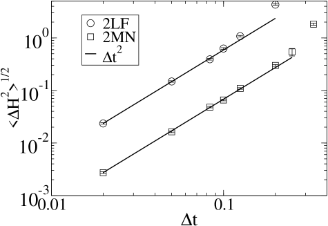
Figure 1: $\langle\Delta H^{2}\rangle^{1/2}$ as a function of $\Delta t$. Simulations are performed at $\beta=5.00$ and $\kappa=0.160$ on $4^{4}$ lattices. The line proportional to $\Delta t^{2}$ is drawn to guide the eye.

Figure 1 shows $\langle\Delta H^{2}\rangle^{1/2}$ as a function of step size $\Delta t$ at $\beta=5.00$ and $\kappa=0.160$ on $4^{4}$ lattices. We see that $\langle\Delta H^{2}\rangle^{1/2}$ is proportional to $\Delta t^{2}$ as expected and the error of the 2MN integrator is about 10 times smaller than that of the 2LF integrator at any $\Delta t$ until instabilities show up.

Figure 2: $C_{2LF}/C_{2MN}$ as a function of $\kappa$. Simulations at $\beta=5.00(5.60)$ are performed on $4^{4}(8^{4})$ lattices.

Figure 2 shows the ratio $C_{2LF}/C_{2MN}$ as a function of $\kappa$. The coefficients $C_{2LF}$ and $C_{2MN}$ are extracted by using eq.(50) for the 2nd order with simulations at a small value of $\Delta t$. As seen in the figure, $C_{2LF}/C_{2MN}$ is about 10, which means that the error of the 2MN integrator is about 10 times smaller than that of the 2LF integrator. This is consistent with the theoretical expectation of Omelyan et al.. If we take $C_{2LF}/C_{2MN}\approx 10$, this means that the step size of the 2MN integrator can be increased by a factor 3 ($\approx\sqrt{10}$) over that of the 2LF integrator, as long as the error still behaves as $\Delta t^{2}$. Since the 2MN integrator has two force calculations per elementary step, the efficiency should be measured by $\displaystyle\sqrt{C_{2LF}/C_{2MN}}/2$, which is about 1.5. Thus it is concluded that the 2MN integrator is about 50% faster than the 2LF integrator.

Of course, this assessment rests on the assumption that the step size can indeed be increased without running into instabilities, so that the limiting factor in the step size comes from the error accumulation. Note that the 2MN integrator appears no worse, or perhaps slightly better, than the 2LF in terms of instabilities: departure from the quadratic behaviour $\langle\Delta H^{2}\rangle^{1/2}\propto\Delta t^{2}$ starts at similar values of $\langle\Delta H^{2}\rangle^{1/2}$ in Fig. 1, and appears more gradual.

3.5 Comparison of 2nd and 4th order MN integrators

The efficiency of higher order integrators should be measured against lower order ones. From the above analysis we know that the 2MN integrator is more efficient than the 2LF integrator. Therefore we compare the 4MN integrator with the 2MN integrator. Assuming eq.(50) the comparison could be done by following the analysis of [4]. However we found a problem with the 4MN integrator. Namely the error of the Hamiltonian $\langle\Delta H^{2}\rangle^{1/2}$ is not simply described by eq.(50) but is dominated by higher order terms in $\Delta t$ already at small $\langle\Delta H^{2}\rangle^{1/2}$. Figure 3 shows $\langle\Delta H^{2}\rangle^{1/2}$ on $8^{4}$ lattices as a function of $\Delta t$. As seen in the figure (left), at a fixed step size the error of the 4MN5FV integrator is about 1000 times smaller than the previously known 4th order integrator (4RC), which is consistent with the theoretical expectation[6]. The expected behavior of $\langle\Delta H^{2}\rangle^{1/2}\approx C_{4}V^{1/2}\Delta t^{4}$, however, is seen only at small $\langle\Delta H^{2}\rangle^{1/2}$. We are only interested in the region of $0.1\leq\langle\Delta H^{2}\rangle^{1/2}\leq 1$ which corresponds to an acceptance of $60\%\sim 95\%$. In this region, $\langle\Delta H^{2}\rangle^{1/2}$ of the 4MN5FV integrator is dominated by higher order terms in $\Delta t$, which results in that $\langle\Delta H^{2}\rangle^{1/2}$ grows rapidly with $\Delta t$. This observation makes the 4MN integrator unattractive on practical lattice sizes.

Although the 4MN4FP integrator seems to be more stable than the 4MN5FV integrator, it also shows the deviation from the $\Delta t^{4}$ line at small $\langle\Delta H^{2}\rangle^{1/2}$ (See Fig.3). Thus compared to the 2MN integrator, the 4MN integrators tested here seem unattractive. As the quark mass $m$ decreases, it is often seen that the integrator becomes unstable[20], because the force increases as $1/m$. In lattice QCD calculations the parameter region of small quark masses is the physically interesting one. In this region the 4MN integrators may easily show instability, which limits their applicability.

At finite temperature, however, the coefficients $C_{n}$ behave differently from those at zero temperature. Typically we expect $C_{n}^{T\neq 0}\leq C_{n}^{T=0}$. Therefore at finite temperature we may be lead to a different conclusion and this must be studied numerically. A numerical test showed that at finite temperature the 4RC integrator performs better than the 2LF integrator on lattices larger than a minimum size[5]. We have made the same test for the 2MN and 4MN5FV integrators on an $18^{3}\times 4$ lattice at $\beta=5.75$ and $\kappa=0.1525$. For the 2MN integrator the acceptance is measured to be about 0.6 at $\Delta t=0.1$ and for the 4MN5FV integrator the acceptance is about 0.8 at $\Delta t=0.37$. These values of the acceptance are close enough to the optimal acceptance given by eq.(53). The gain of the 4MN5FV integrator over the 2MN one is calculated by

$$G=\frac{(P_{acc}\times\Delta t)_{4th}}{\kappa_{42}(P_{acc}\times\Delta t)_{2nd}},$$ (54)

where $\kappa_{42}$ is the relative cost factor and $\kappa_{42}=2.5$ for the 2MN and 4MN5FV integrators. Substituting the measured values into $G$, $G$ is calculated to be $\approx 2$, which shows that the 4MN5FV integrator is more effective. Thus at finite temperature there is room to use a 4MN integrator depending on the simulation parameters.

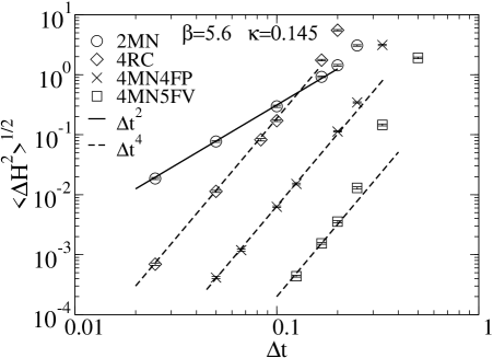
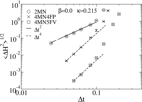
Figure 3: $\langle\Delta H^{2}\rangle^{1/2}$ as a function of $\Delta t$. Simulations are performed on $8^{4}$ lattices. 4RC stands for the 4th order integrator obtained by eq.(24). The lines proportional to $\Delta t^{n}$ are drawn to guide the eye.

4 Tuning the 2MN integrator

The strategy to minimize eqs.(30) and (31) is based on the assumption that the errors coming from the two commutators $[T,[V,T]]$ and $[V,[V,T]]$ are equally dominant. In general this simplifying assumption does not hold. Here we try to minimize a more general form of the error function. Let us assume the following form of $\langle\Delta H^{2}\rangle^{1/2}$,

$$\langle\Delta H^{2}\rangle^{1/2} \approx \sqrt{\alpha(\lambda)^{2}f(\Delta t)^{2}+\beta(\lambda)^{2}g(\Delta t)^{2}},$$ (55)

$$= \sqrt{\alpha(\lambda)^{2}f^{2}+\beta(\lambda)^{2}g^{2}}\Delta t^{2},$$ (56)

where $\alpha(\lambda)$ and $\beta(\lambda)$ are given by eqs.(34) and (35), and $f^{2}$ and $g^{2}$ are unknown parameters, to be determined from numerical simulations. In general, by performing simulations at two values of $\lambda$ one can determine $f^{2}$ and $g^{2}$ numerically. The determination can be made easier by noticing that $\alpha(\lambda_{1})$ and $\beta(\lambda_{2})$ are zero at $\lambda_{1}=(1-1/\sqrt{3})/2$ and $\lambda_{2}=1/6$ respectively. By simulating at $\lambda_{1}$ and $\lambda_{2}$ we immediately obtain $f^{2}$ and $g^{2}$.

Figure 4 shows $\langle\Delta H^{2}\rangle^{1/2}$ at $\beta=5.00$ and $\kappa=0.160$ as a function of $\lambda$. We see that the optimal $\lambda$ at the minimum of $\langle\Delta H^{2}\rangle^{1/2}$ is slightly different from $\lambda_{c}$, the value of eq.(33). Moreover the optimal $\lambda$ is different between the velocity and position version integrators. Here eq.(32) is the position version integrator. The velocity version is obtained by interchanging $T$ and $V$ in eq.(32). The lines in the figure are given by eq.(56), with $f^{2}$ and $g^{2}$ determined by simulations of the position version of 2MN integrator at $\lambda_{1}$ and $\lambda_{2}$. To draw the dashed line for the velocity version, we simply interchange the values $f^{2}$ and $g^{2}$. Both lines describe the numerical results very well, down to $\lambda=0$. Note that the velocity version of 2MN integrator becomes the position version of 2LF integrator at $\lambda=0$, and vice versa. The position version of the 2MN integrator gives a slightly smaller minimum. At $\lambda=0$ the velocity version of 2MN integrator has a smaller error than the position version, which means that the position version of 2LF integrator has a smaller error than the velocity version. This was already observed in [21]. Since the position version also leads to one less force evaluation by the end of a trajectory, we definitely recommend using the position version (for the 2MN and the 2LF integrators both): it requires less work and gives a higher acceptance.

The quality of our fit justifies a posteriori the ansatz made for the magnitude of the error eq.(56). Indeed, to leading order $\Delta t^{4}$, the error $\langle\Delta H^{2}\rangle$ should be of the form

$$\langle\Delta H^{2}\rangle=(\alpha(\lambda)^{2}\langle F^{2}\rangle+\alpha(\lambda)\beta(\lambda)\langle FG+GF\rangle+\beta(\lambda)^{2}\langle G^{2}\rangle)\Delta t^{4},$$ (57)

where $F=[T,[V,T]]$ and $G=[V,[V,T]]$ from eq.(28). We find that the crossterm $\langle FG\rangle$ is in our case ”one order of magnitude smaller” than $\langle F^{2}\rangle$ and $\langle G^{2}\rangle$, indicating that the two operators are almost uncorrelated in our system. While this finding may not be true in general, it provides support for the minimum norm strategy of Omelyan et al. at least in the context of lattice QCD.

Figure 5 shows $|f|\Delta t^{2}$, $|g|\Delta t^{2}$ and $|f|/|g|$ as a function of $1/\kappa$ at $\beta=5.00$ on $4^{4}$ lattices ($\Delta t=0.05)$. As one approaches $\kappa_{c}$, both $|f|$ and $|g|$ increase. On the other hand the ratio $|f|/|g|$ decreases. This is as expected since $g$ comes from the error term $[V,[V,T]]$ involving two factors of the fermion potential, versus one for $f$ and $[T,[V,T]]$. Although $|f|/|g|$ seems to approach one at $\kappa_{c}$, there is a possibility that it further goes down to zero and its limit must be carefully investigated. Note that when $|f|/|g|=1$, the optimal $\lambda$ becomes $\lambda_{c}$.

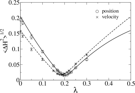
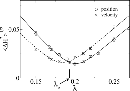
Figure 4: $\langle\Delta H^{2}\rangle^{1/2}$ as a function of $\lambda$. The right figure is a zoom of the left. Simulations are performed at $\beta=5.00$ and $\kappa=0.160$ on $4^{4}$ lattices with $\Delta t=0.05$. The lines are determined from simulations of the position version integrator at $\lambda_{1}$ and $\lambda_{2}$. The position version has a small advantage over the velocity version, since it gives a slightly reduced minimum RMS error (right).

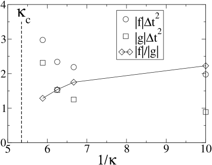
Figure 5: $|f|\Delta t^{2}$, $|g|\Delta t^{2}$ and $|f|/|g|$ as a function of $1/\kappa$. Simulations are performed at $\beta=5.00$ on $4^{4}$ lattices with $\Delta t=0.05$. The dashed line indicates $\kappa_{c}=0.187$[19].

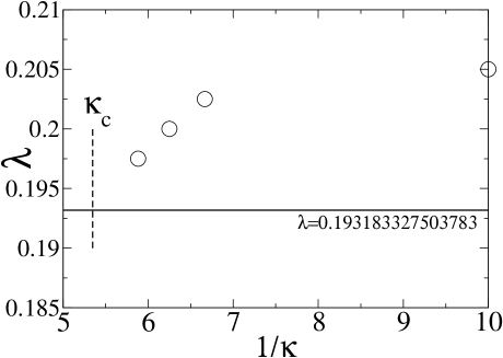
Figure 6: Optimal $\lambda$ as a function of $1/\kappa$. Simulations are performed at $\beta=5.00$ on $4^{4}$ lattices with $\Delta t=0.05$. The dashed line indicates $\kappa_{c}=0.187$.

Figure 6 shows the optimal $\lambda$ as a function of $1/\kappa$. We see that the optimal $\lambda$ is different from $\lambda_{c}$ and slightly larger.

5 Conclusions

We have tested the new 2nd and 4th order integrators obtained by minimizing the norm of the error coefficients. We find that the 2MN integrator performs better than the conventional 2LF integrator, by about 50%. Therefore we recommend to use the 2MN integrator in HMC simulations. Although in our tests we used the standard Wilson fermion action, the 2MN integrator can be used for any actions, e.g, KS fermions, improved actions, polynomial actions for odd flavors[22, 23]. Moreover we may combine the 2MN integrator with other acceleration techniques such as multiple time step integration[9], multiple pseudo-fermions[24] and preconditioned actions[23].

The same 2MN integrator can also be used in the Trotter-Suzuki decomposition of the partition function: $\exp(-\beta H)=(\exp(-\Delta t~{}H))^{N}$, where $N=\beta/\Delta t$, in Quantum Monte Carlo simulations, when a formulation in continuous imaginary time [25] is not practical.

Although at first sight, one can equivalently start by integrating over positions or velocities, we observe that integrating over positions first gives a slightly higher acceptance [21], with one less force evaluation at the end of a trajectory.

References

- [1] S. Duane, A. D. Kennedy, B. J. Pendleton and D. Roweth, Phys. Lett. B 195 (1987) 216.
- [2] M. Campostrini and P. Rossi, Nucl. Phys. B 329 (1990) 753.
- [3] M. Creutz and A. Gocksch, Phys. Rev. Lett. 63 (1989) 9.
- [4] T. Takaishi, Comput. Phys. Commun. 133 (2000) 6 [arXiv:hep-lat/9909134].
- [5] T. Takaishi, Phys. Lett. B 540 (2002) 159 [arXiv:hep-lat/0203024].
- [6] I.P. Omelyan, I.M. Mryglod and R. Folk, Comput. Phys. Commun. 151 (2003) 272.
- [7] E. Forest and R. D. Ruth, PhysicaD 43 (1990) 105.
- [8] H. Yoshida, Phys. Lett. A 150 (1990) 262.
- [9] J. C. Sexton and D. H. Weingarten, Nucl. Phys. B 380 (1992) 665.
- [10] M. Suzuki, Phys. Lett. A 146 (1990) 319.
- [11] M. Suzuki, J. Math. Phys. 32 (1991) 400.
- [12] M. Suzuki, Phys. Lett. A 201 (1995) 425.
- [13] S.A. Chin, Phys. Lett. A 226 (1997) 344.
- [14] A.D. Kennedy, “Monte Carlo algorithms and non-local actions”, in Fields Institute Communications, vol. 26 (American Mathematical Society pub., 2000).
- [15] I.P. Omelyan, I.M. Mryglod and R. Folk, Phys. Rev. E 65 (2002) 056706.
- [16] K.G. Wilson, Phys. Rev. D 10 (1974) 2445.
- [17] S. Gupta, A. Irback, F. Karsch and B. Petersson, Phys. Lett. B 242 (1990) 437.
- [18] M. Creutz, Phys. Rev. D 38 (1988) 1228.
- [19] A.Ukawa, Nucl. Phys. B (Proc. Suppl.) 10 (1989) 66.
- [20] See e.g., A.D. Kennedy, hep-lat/0409167
- [21] R. Gupta, G. W. Kilcup and S. R. Sharpe, Phys. Rev. D 38 (1988) 1278.
- [22] T. Takaishi and P. de Forcrand, Int. J. Mod. Phys. C 13 (2002) 343 [arXiv:hep-lat/0108012].
- [23] P. de Forcrand and T. Takaishi, Nucl. Phys. Proc. Suppl. 53 (1997) 968 [arXiv:hep-lat/9608093].
- [24] M. Hasenbusch, Phys. Lett. B 519 (2001) 177 [arXiv:hep-lat/0107019].
- [25] B.B. Beard and U.J. Wiese, Nucl. Phys. Proc. Suppl. 53 (1997) 838 [arXiv:cond-mat/9602164].