DESY 05-029 Edinburgh 2005/03 Leipzig LU-ITP 2005/014 Liverpool LTH 648 Renormalisation of one-link quark operators for overlap fermions with Lüscher-Weisz gauge action

Abstract

We compute lattice renormalisation constants of one-link quark operators (i.e. operators with one covariant derivative) for overlap fermions and Lüscher-Weisz gauge action in one-loop perturbation theory. Among others, such operators enter the calculation of moments of polarised and unpolarised hadron structure functions. Results are given for $\beta=8.45$, $\beta=8.0$ and mass parameter $\rho=1.4$, which are commonly used in numerical simulations. We apply mean field (tadpole) improvement to our results.

1 Introduction

In a recent publication [1] we have computed lattice renormalisation constants of local bilinear quark operators for overlap fermions and improved gauge actions in one-loop perturbation theory. Among the actions we considered were the Symanzik, Lüscher-Weisz, Iwasaki and DBW2 gauge actions. The results were given for a variety of $\rho$ parameters. Furthermore, we showed how to apply mean field (tadpole) improvement to overlap fermions. In this letter we shall extend our work to one-link bilinear quark operators. Operators of this kind enter, for example, the calculation of moments of polarised and unpolarised hadron structure functions. The present calculations are much more involved than the previous ones, so that we shall restrict ourselves to the Lüscher-Weisz action, and to parameters actually being used in numerical calculations.

The integral part of the overlap fermion action [2, 3, 4]

$$S_{F}=\bar{\psi}\left[\left(1-\frac{am}{2}\right)D_{N}+m\right]\psi\,,$$ (1)

$m$ being the mass of the quark, is the Neuberger-Dirac operator

$$D_{N}=\frac{\rho}{a}\left(1+\frac{X}{\sqrt{X^{\dagger}X}}\right)\,,\;X=D_{W}-\frac{\rho}{a}\,,$$ (2)

where $D_{W}$ is the Wilson-Dirac operator, and $\rho$ is a real parameter corresponding to a negative mass term. At tree level $0<\rho<2r$, where $r$ is the Wilson parameter. We take $r=1$ and consider massless quarks.

Numerical simulations of overlap fermions are significantly more costly than simulations of Wilson fermions. The cost of overlap fermions is largely determined by the condition number of $X^{\dagger}X$. This number is greatly reduced for improved gauge field actions [5]. For example, for the tadpole improved Lüscher-Weisz action we found a reduction factor of $\gtrsim 3$ compared to the Wilson gauge field action [6]. The reason is that the Lüscher-Weisz action suppresses unphysical zero modes, sometimes called dislocations [7]. A reduction of the number of small modes of $X^{\dagger}X$ appears also to result in an improvement of the locality of the overlap operator [5].

We consider the tadpole improved Lüscher-Weisz action [8, 9, 10]

$$\begin{split}S_{G}&=\frac{6}{g^{2}}\,\,\Bigg{[}c_{0}\sum_{\rm plaquette}\frac{1}{3}\,{\rm Re\,Tr\,}(1-U_{\rm plaquette})\,+\,c_{1}\sum_{\rm rectangle}\frac{1}{3}\,{\rm Re\,Tr\,}(1-U_{\rm rectangle})\\ &\phantom{=}+\,c_{3}\sum_{\rm parallelogram}\frac{1}{3}\,{\rm Re\,Tr\,}(1-U_{\rm parallelogram})\Bigg{]}\,,\end{split}$$ (3)

where $U_{\rm plaquette}$ is the standard plaquette, $U_{\rm rectangle}$ denotes the loop of link matrices around the $1\times 2$ rectangle, and $U_{\rm paralellogram}$ denotes the loop along the edges of the three-dimensional cube. It is required that $c_{0}+8c_{1}+8c_{3}=1$ in the limit $g\rightarrow 0$, in order to ensure the correct continuum limit. We define

$$\beta=\frac{6}{g^{2}}\,c_{0}\,.$$ (4)

The remaining parameters are [10]:

$$\frac{c_{1}}{c_{0}}=-\frac{(1+0.4805\,\alpha)}{20\,u_{0}^{2}}\,,\quad\frac{c_{3}}{c_{0}}=-\frac{0.03325\,\alpha}{u_{0}^{2}}\,,\quad\frac{1}{c_{0}}=1+8\left(\frac{c_{1}}{c_{0}}+\frac{c_{3}}{c_{0}}\right)\,,$$ (5)

where

$$u_{0}=\left(\frac{1}{3}\,{\rm Tr}\,\langle U_{\rm plaquette}\rangle\right)^{\frac{1}{4}}\,,\quad\alpha=-\frac{\log(u_{0}^{4})}{3.06839}\,.$$ (6)

The final results cannot be expressed in analytic form (as a function of $\beta$ and $\rho$) anymore. We therefore have to make a choice. Here we consider two couplings, $\beta=8.45$ and $8.0$, at which we run Monte Carlo simulations at present [6, 11]. The corresponding values of $c_{1}$ and $c_{3}$ are [12]:

$$\beta$$

8.45 -0.154846 -0.0134070 5.29(7)

8.00 -0.169805 -0.0163414 3.69(4)

(7)

In (7) we also quote the corresponding force parameters $r_{0}/a$, as given in [12]. Assuming that $r_{0}=0.5\,\mbox{fm}$, they translate into a lattice spacing of $a=0.095\,\mbox{fm}$ at $\beta=8.45$ and $a=0.136\,\mbox{fm}$ at $\beta=8.0$. The mass parameter was chosen to be $\rho=1.4$. This appeared to be a fair compromise between optimising the condition number of $X^{\dagger}X$ as well as the locality properties of $D_{N}$ [13].

The paper is organised as follows. In Section 2 we give a brief outline of our calculations and present results for the renormalisation constants in one-loop perturbation theory. In Section 3 we tadpole improve our results, and in Section 4 we give our conclusions.

2 Outline of the calculation and one-loop results

The Feynman rules specific for overlap fermions [14, 15] are collected in [1], while the gluon-operator and the gluon-gluon-operator vertices (needed for the cockscomb and operator tadpole diagrams) are independent of the fermion action and can be found in [16]. We consider general covariant gauges, specified by the gauge parameter $\xi$. The Landau gauge corresponds to $\xi=1$, while the Feynman gauge corresponds to $\xi=0$. In lattice momentum space the gluon propagator $D_{\mu\nu}(k)$ is given by the set of linear equations

$$\sum_{\rho}\left[G_{\mu\rho}(k)-\frac{\xi}{\xi-1}\hat{k}_{\mu}\hat{k}_{\rho}\right]D_{\rho\nu}(k)=\delta_{\mu\nu}\,,$$ (8)

where

$$G_{\mu\nu}(k)=\hat{k}_{\mu}\hat{k}_{\nu}+\sum_{\rho}\left(\hat{k}_{\rho}^{2}\delta_{\mu\nu}-\hat{k}_{\mu}\hat{k}_{\rho}\delta_{\rho\nu}\right)\,d_{\mu\rho}$$ (9)

and

$$d_{\mu\nu}=\left(1-\delta_{\mu\nu}\right)\left[C_{0}-C_{1}\,a^{2}\hat{k}^{2}-C_{2}\,a^{2}(\hat{k}_{\mu}^{2}+\hat{k}_{\nu}^{2})\right]\,,\quad\hat{k}_{\mu}=\frac{2}{a}\sin\frac{ak_{\mu}}{2}\,,\quad\hat{k}^{2}=\sum_{\mu}\hat{k}_{\mu}^{2}\,.$$ (10)

The coefficients $\{C_{i}\}$ are related to the coefficients $\{c_{i}\}$ of the improved action by

$$C_{0}=c_{0}+8c_{1}+8c_{3}\,,\,\,\,C_{1}=c_{3}\,,\,\,\,C_{2}=c_{1}-c_{3}\,.$$ (11)

The calculations are done analytically as far as this is possible using Mathematica. Part of the numerical results have been checked by an independent routine.

The bare lattice operators $\mathcal{O}(a)$ are, in general, divergent as $a\rightarrow 0$. We define finite renormalised operators by

$$\mathcal{O}^{\mathcal{S}}(\mu)=Z_{\mathcal{O}}^{\mathcal{S}}(a,\mu)\,\mathcal{O}(a)\,,$$ (12)

where $\mathcal{S}$ denotes the renormalisation scheme. We have assumed that the operators do not mix under renormalisation, which is the case for the operators considered in this letter. The renormalisation constants $Z_{\mathcal{O}}$ are often determined in the $MOM$ scheme first from the gauge fixed quark propagator $S_{N}$ and the amputated Green function $\Lambda_{\mathcal{O}}$ of the operator $\mathcal{O}$:

$$Z_{\psi}^{MOM}(a,\mu)\;S_{N}\;\big{|}_{p^{2}=\mu^{2}} = S^{\rm tree}\,,$$ (13)

$$\frac{Z^{MOM}_{\cal O}(a,\mu)}{Z^{MOM}_{\psi}(a,\mu)}\;\Lambda_{\cal O}\;\big{|}_{p^{2}=\mu^{2}} = \Lambda_{\cal O}^{\rm tree}+{\rm\ other\ Dirac\ structures}\,.$$ (14)

(Note that $Z_{\psi}=1/Z_{2}$.) The renormalisation constants can be converted to the ${\overline{MS}}$ scheme,

$$\begin{split}Z_{\psi}^{{\overline{MS}}}(a,\mu)&=Z_{\psi}^{{\overline{MS}},MOM}Z_{\psi}^{MOM}(a,\mu)\,,\\ Z_{\mathcal{O}}^{{\overline{MS}}}(a,\mu)&=Z_{\mathcal{O}}^{{\overline{MS}},MOM}Z_{\mathcal{O}}^{MOM}(a,\mu)\,,\end{split}$$ (15)

where $Z_{\psi}^{{\overline{MS}},MOM}$, $Z_{\mathcal{O}}^{{\overline{MS}},MOM}$ are calculable in continuum perturbation theory, and therefore are independent of the particular choice of lattice gauge and fermion actions.

In [1] the wave function renormalisation constants where found to be

$$Z_{\psi}^{MOM}(a,\mu)=1-\frac{g^{2}C_{F}}{16\pi^{2}}\,\left[2(1-\xi)\log(a\mu)+4.79201\,\xi+b_{\Sigma}\right]$$ (16)

in the $MOM$ scheme, and

$$Z_{\psi}^{{\overline{MS}}}(a,\mu)=1-\frac{g^{2}C_{F}}{16\pi^{2}}\,\left[2(1-\xi)\log(a\mu)+3.79201\,\xi+b_{\Sigma}+1\right]$$ (17)

in the ${\overline{MS}}$ scheme, with $C_{F}=4/3$ and

$$\beta$$

8.45 -17.429

8.00 -17.054

(18)

We consider the following one-link operators

$${\cal O}_{\mu\nu} = \frac{i}{2}\,\bar{\psi}(x)\gamma_{\mu}\stackrel{{\scriptstyle\leftrightarrow}}{{D}}_{\nu}\psi(x)\,,$$ (19)

$${\cal O}_{\mu\nu}^{5} = \frac{i}{2}\,\bar{\psi}(x)\gamma_{\mu}\gamma_{5}\stackrel{{\scriptstyle\leftrightarrow}}{{D}}_{\nu}\psi(x)\,,$$ (20)

where $\stackrel{{\scriptstyle\leftrightarrow}}{{D}}_{\nu}=\stackrel{{\scriptstyle\rightarrow}}{{D}}_{\nu}-\stackrel{{\scriptstyle\leftarrow}}{{D}}_{\nu}$ is the (symmetric) lattice covariant derivative. While in our previous work [1], which involved local bilinear quark operators, we only had to deal with the vertex diagram shown on the left-hand side of Fig. 1, we now obtain contributions from additional diagrams: the operator tadpole and the cockscomb diagrams shown on the right-hand side of Fig. 1.

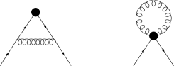
Figure 1: The one-loop lattice Feynman diagrams contributing to the amputated Green function. From left to right: vertex, operator tadpole and cockscomb diagrams.

The amputated Green function of the operator ${\cal O}_{\mu\nu}$ [eq. (19)] turns out to be

$$\Lambda_{\mu\nu}(a,p) = \gamma_{\mu}p_{\nu}+\frac{g^{2}C_{F}}{16\pi^{2}}\bigg{\{}\left[\left(\frac{1}{3}+\xi\right)\log(a^{2}p^{2})-4.29201\,\xi+b_{1}\right]\gamma_{\mu}p_{\nu}$$

$$+\left[\frac{4}{3}\log(a^{2}p^{2})+\frac{1}{2}\,\xi+b_{2}\right]\gamma_{\nu}p_{\mu}+\left[-\frac{2}{3}\log(a^{2}p^{2})-\frac{1}{2}\,\xi+b_{3}\right]\delta_{\mu\nu}\not{p}$$

$$+\,b_{4}\,\delta_{\mu\nu}\gamma_{\nu}p_{\nu}+\left(-\frac{4}{3}+\xi\right)\frac{p_{\mu}p_{\nu}}{p^{2}}\not{p}\bigg{\}}\,,$$

where $p$ is the external quark momentum, and the coefficients $\{b_{i}\}$ are given in Table 1 for the tadpole improved Lüscher-Weisz action and, for comparison, for the plaquette action (with $c_{1}=c_{3}=0$) as well.

Action	$b_{1}$	$b_{2}$	$b_{3}$	$b_{4}$
$\beta=8.45$	-05.6115	-3.8336	2.7793	0.3446
$\beta=8.0\phantom{0}$	-05.2883	-3.7636	2.7310	0.3331
Plaquette	-10.6882	-4.7977	3.4612	0.5267

Table 1: The coefficients $\{b_{i}\}$ for the tadpole improved Lüscher-Weisz action at $\beta=8.45$ and $8.0$, as well as for plaquette action.

The latter numbers are independent of $\beta$. The Green function $\Lambda_{\mu\nu}^{5}(a,p)$ of the operator ${\cal O}_{\mu\nu}^{5}$ [eq. (20)] is obtained by multiplying the right-hand side of (2) by $\gamma_{5}$ from the right. The coefficients $\{b_{i}^{5}\}$ turn out to be identical to $\{b_{i}\}$, as is expected for overlap fermions. Thus, ${\cal O}_{\mu\nu}$ and ${\cal O}_{\mu\nu}^{5}$ have the same renormalisation constants. In the following we may therefore restrict ourselves to the operator ${\cal O}_{\mu\nu}$.

It has been checked numerically that the gauge dependent part of (2) is universal (i.e. independent of the lattice gauge and fermion action), in accordance with the arguments presented in [1].

Under the hypercubic group $H(4)$ the 16 operators of type (19) fall into the following four irreducible representations [17]:

$$\tau_{3}^{(6)}:\quad{\cal O}_{v_{2a}} \equiv \frac{1}{2}\left({\cal O}_{14}+{\cal O}_{41}\right)\,,$$ (22)

$$\tau_{1}^{(3)}:\quad{\cal O}_{v_{2b}} \equiv {\cal O}_{44}-\frac{1}{3}\left({\cal O}_{11}+{\cal O}_{22}+{\cal O}_{33}\right)\,,$$ (23)

$$\tau_{1}^{(1)}:\quad{\cal O}_{v_{2c}} \equiv {\cal O}_{11}+{\cal O}_{22}+{\cal O}_{33}+{\cal O}_{44}\,,$$ (24)

$$\tau_{1}^{(6)}:\quad{\cal O}_{v_{2d}} \equiv {\cal O}_{14}-{\cal O}_{41}\,.$$ (25)

(We have given one example operator in each representation. A complete basis for each representation can be found in [17].) The operators (22) and (23) are widely used in numerical simulations [18, 19, 6, 11]. They correspond to the first moment of the parton distribution. The operators (24) and (25) represent higher twist contributions in the operator product expansion, and so are not used as much as operators in the first two representations. For completeness we give results for all four representations, so that the renormalisation factors for all operators of the form (19) will be known. We denote the corresponding amputated Green functions by $\Lambda_{v_{2a}}$, $\Lambda_{v_{2b}}$, $\Lambda_{v_{2c}}$ and $\Lambda_{v_{2d}}$. From (2) we read off

$$\Lambda_{v_{2a}}\!\! = \!\frac{1}{2}\Big{(}\gamma_{1}p_{4}+\gamma_{4}p_{1}\Big{)}\,\left\{1+\frac{g^{2}C_{F}}{16\pi^{2}}\left[(\xi+\frac{5}{3})\,\log(a^{2}p^{2})-3.79201\,\xi+b_{v_{2a}}\right]\right\}$$ (26)

$$\!+\frac{g^{2}C_{F}}{16\pi^{2}}\left(-\frac{4}{3}+\xi\right)\frac{p_{1}p_{4}}{p^{2}}\not{p}\,,$$

$$\Lambda_{v_{2b}}\!\! = \!\Big{(}\gamma_{4}p_{4}-\frac{1}{3}\sum_{i=1}^{3}\gamma_{i}p_{i}\Big{)}\,\left\{1+\frac{g^{2}C_{F}}{16\pi^{2}}\left[(\xi+\frac{5}{3})\,\log(a^{2}p^{2})-3.79201\,\xi+b_{v_{2b}}\right]\right\}$$ (27)

$$\!+\frac{g^{2}C_{F}}{16\pi^{2}}\left(-\frac{4}{3}+\xi\right)\left(p_{4}^{2}-\frac{1}{3}\sum_{i=1}^{3}p_{i}^{2}\right)\frac{\not{p}}{p^{2}}\,,$$

$$\Lambda_{v_{2c}}\!\! = \!\not{p}\,\left\{1+\frac{g^{2}C_{F}}{16\pi^{2}}\left[(\xi-1)\,\log(a^{2}p^{2})-4.79201\,\xi+b_{v_{2c}}\right]\right\}\,,$$ (28)

$$\Lambda_{v_{2d}}\!\! = \!\Big{(}\gamma_{1}p_{4}-\gamma_{4}p_{1}\Big{)}\,\left\{1+\frac{g^{2}C_{F}}{16\pi^{2}}\left[(\xi-1)\,\log(a^{2}p^{2})-4.79201\,\xi+b_{v_{2d}}\right]\right\}$$ (29)

with

$$b_{v_{2a}}=b_{1}+b_{2}\,,\quad b_{v_{2b}}=b_{1}+b_{2}+b_{4}\,,\quad b_{v_{2c}}=b_{1}+b_{2}+4\,b_{3}+b_{4}-\frac{4}{3}\,,\quad b_{v_{2d}}=b_{1}-b_{2}\,.$$ (30)

It is worth pointing out that with Wilson or clover fermions the Green functions $\Lambda_{v_{2c}}$ and $\Lambda_{v_{2d}}$ both show perturbative mixing of $O(g^{2}/a)$ with local operators. With overlap fermions these $O(1/a)$ terms are completely absent, showing once again that overlap fermions behave much more like continuum fermions when mixing is a possibility.

Using (14) and (16), we obtain the renormalisation constants in the $MOM$ scheme:

$$Z_{v_{2a},v_{2b}}^{MOM}(a,\mu) = 1-\frac{g^{2}C_{F}}{16\pi^{2}}\left[\frac{16}{3}\log(a\mu)+\xi+b_{v_{2a},v_{2b}}+b_{\Sigma}\right]\,,$$ (31)

$$Z_{v_{2c},v_{2d}}^{MOM}(a,\mu) = 1-\frac{g^{2}C_{F}}{16\pi^{2}}\left[\,b_{v_{2c},v_{2d}}+b_{\Sigma}\,\right]\,.$$ (32)

As already mentioned, the conversion factors $Z_{v_{2a},v_{2b},v_{2c},v_{2d}}^{{\overline{MS}},MOM}$ are universal [16]. They are given by

$$Z_{v_{2a},v_{2b}}^{{\overline{MS}},MOM} = 1-\frac{g^{2}C_{F}}{16\pi^{2}}\,\left(\frac{40}{9}-\xi\right)\,,$$ (33)

$$Z_{v_{2c}}^{{\overline{MS}},MOM} = 1-\frac{g^{2}C_{F}}{16\pi^{2}}\,\left(-\frac{4}{3}\right)\,,$$ (34)

$$Z_{v_{2d}}^{{\overline{MS}},MOM} = 1\,.$$ (35)

In the ${\overline{MS}}$ scheme we then find

$$Z_{v_{2a},v_{2b}}^{{\overline{MS}}}(a,\mu) = 1-\frac{g^{2}C_{F}}{16\pi^{2}}\left[\frac{16}{3}\log(a\mu)+\frac{40}{9}+b_{v_{2a},v_{2b}}+b_{\Sigma}\right]\,,$$ (36)

$$Z_{v_{2c}}^{{\overline{MS}}}(a,\mu) = 1-\frac{g^{2}C_{F}}{16\pi^{2}}\left[-\frac{4}{3}+b_{v_{2c}}+b_{\Sigma}\right]\,,$$ (37)

$$Z_{v_{2d}}^{{\overline{MS}}}(a,\mu) = 1-\frac{g^{2}C_{F}}{16\pi^{2}}\left[b_{v_{2d}}+b_{\Sigma}\right]\,.$$ (38)

3 Tadpole improved results

A detailed discussion of mean field – or tadpole – improvement for overlap fermions and extended gauge actions has been given in [1]. Here we will briefly recall the basic idea, before presenting our results.

Tadpole improved renormalisation constants are defined by

$$Z_{\mathcal{O}}^{TI}=Z_{\mathcal{O}}^{MF}\left(\frac{Z_{\mathcal{O}}}{Z_{\mathcal{O}}^{MF}}\right)_{\rm pert}\,,$$ (39)

where $Z_{\mathcal{O}}^{MF}$ is the mean field approximation of $Z_{\mathcal{O}}$, while the right-hand factor is computed in perturbation theory. For overlap fermions (with $r=1$), and operators with $n_{D}$ covariant derivatives, we have

$$Z_{\cal O}^{MF}=\frac{\rho\,u_{0}^{1-n_{D}}}{\rho-4(1-u_{0})}\,.$$ (40)

In our case $n_{D}=1$. It is required that $\rho>4(1-u_{0})$, which is fulfilled here (see Table 2).

$\beta$	$k_{u}^{TI}$	$u_{0}^{4}$
8.45	0.543338 $\pi^{2}$	0.65176
8.00	0.515069 $\pi^{2}$	0.62107

Table 2: The coefficient $k_{u}^{TI}$ and the average plaquette $u_{0}^{4}$ at $\beta=8.45$ and $8.0$.

To compute the right-hand factor in (39), we have to remove the tadpole contributions from the perturbative expressions of $Z_{\cal O}$ first. This is achieved if we re-express the perturbative series in terms of tadpole improved coefficients:

$$\frac{c_{0}^{TI}}{g_{TI}^{2}}=u_{0}^{4}\;\frac{c_{0}}{g^{2}}\,,\quad\quad\frac{c_{i}^{TI}}{g_{TI}^{2}}=u_{0}^{6}\;\frac{c_{i}}{g^{2}}\,,\quad i=1,3\,.$$ (41)

This does not fix all parameters, but leaves us with some freedom of choice. The simplest choice is to define

$$g_{TI}^{2}=\frac{g^{2}}{u_{0}^{4}}\,,\quad\quad c_{0}^{TI}=c_{0}\,,\quad\quad c_{i}^{TI}=u_{0}^{2}\,c_{i}\,,\quad i=1,3\,.$$ (42)

With this choice

$$C_{0}^{TI}=c_{0}+8c_{1}^{TI}+8c_{3}^{TI}\,,\quad C_{1}^{TI}=u_{0}^{2}\,C_{1}\,,\quad C_{2}^{TI}=u_{0}^{2}\,C_{2}\,.$$ (43)

(Note that $C_{0}^{TI}\neq 1$. However, $C_{0}^{TI}\rightarrow 1$ in the continuum limit.) This means that we have to replace every $g^{2}$ by $g_{TI}^{2}$ and every $c_{1}$ and $c_{3}$ by $c_{1}^{TI}$ and $c_{3}^{TI}$, respectively, while keeping $c_{0}$ unchanged. The effect of introducing tadpole improved coefficients (42) is that the rescaled gluon propagator remains of the same form as we change $u_{0}$, thus ensuring fast convergence.

To compute $Z_{\cal O}^{MF}$ perturbatively, we need to know the perturbative expansion of $u_{0}$ to one-loop order [20, 10]. We write

$$u_{0}=1-\frac{g_{TI}^{2}C_{F}}{16\pi^{2}}\,k_{u}^{TI}\,.$$ (44)

In [1] we have computed $k_{u}^{TI}$ for the Lüscher-Weisz action with coefficients $C_{0}^{TI}$, $C_{1}^{TI}$ and $C_{2}^{TI}$. The numbers are given in Table 2 for our two values of $\beta$, together with the ‘measured’ values of $u_{0}^{4}$. Expanding (40) then gives

$$Z_{\cal O\,{\rm pert}}^{MF}=1+\frac{g_{TI}^{2}C_{F}}{16\pi^{2}}\,\frac{4}{\rho}k_{u}^{TI}\,.$$ (45)

Let us now rewrite the one-loop renormalisation constants of Section 2 as

$$Z_{v_{2a},v_{2b}} = 1-\frac{C_{F}\,g^{2}}{16\pi^{2}}\left[\frac{16}{3\,C_{0}}\log(a\mu)+B_{v_{2a},v_{2b}}(\rho,C)\right]\,,$$ (46)

$$Z_{v_{2c},v_{2d}} = 1-\frac{C_{F}\,g^{2}}{16\pi^{2}}B_{v_{2c},v_{2d}}(\rho,C)\,.$$ (47)

Dividing (46) and (47) by (45) and inserting (40), we obtain mean field/tadpole improved renormalisation constants:

$$Z_{v_{2a},v_{2b}}^{TI} = \frac{\rho}{\rho-4(1-u_{0})}\left\{1-\frac{g_{TI}^{2}C_{F}}{16\pi^{2}}\left[\frac{16}{3\,C^{TI}_{0}}\log(a\mu)+B_{v_{2a},v_{2b}}^{TI}\right]\right\}\,,$$ (48)

$$Z_{v_{2c},v_{2d}}^{TI} = \frac{\rho}{\rho-4(1-u_{0})}\left\{1-\frac{g_{TI}^{2}C_{F}}{16\pi^{2}}B_{v_{2c},v_{2d}}^{TI}\right\}\,,$$ (49)

where we have introduced the abbreviated notation

$$B^{TI}=B(\rho,C^{TI})+\frac{4}{\rho}\,k_{u}^{TI}\,.$$ (50)

The coefficients $B(\rho,C^{TI})$ are the analogue of $B(\rho,C)$, with $C_{0}$, $C_{1}$ and $C_{2}$ being replaced by $C_{0}^{TI}$, $C_{1}^{TI}$ and $C_{2}^{TI}$, respectively. In (48) and (49) only the gluon propagator has been tadpole improved.

To tadpole improved the fermion propagator as well, we must replace $\rho$ by [1]

$$\rho^{TI}=\frac{\rho-4(1-u_{0})}{u_{0}}$$ (51)

in the right-hand perturbative factor of (39). This defines ‘fully tadpole improved’ renormalisation constants

$$Z_{v_{2a},v_{2b}}^{FTI} = \frac{\rho}{\rho-4(1-u_{0})}\left\{1-\frac{g_{TI}^{2}C_{F}}{16\pi^{2}}\left[\frac{16}{3\,C^{TI}_{0}}\log(a\mu)+B_{v_{2a},v_{2b}}^{FTI}\right]\right\}\,,$$ (52)

$$Z_{v_{2c},v_{2d}}^{FTI} = \frac{\rho}{\rho-4(1-u_{0})}\left\{1-\frac{g_{TI}^{2}C_{F}}{16\pi^{2}}B_{v_{2c},v_{2d}}^{FTI}\right\}$$ (53)

with

$$B^{FTI}=B(\rho^{TI},C^{TI})+\frac{4}{\rho^{TI}}\,k_{u}^{TI}\,.$$ (54)

In Table 3 we present our final results and compare tadpole improved and unimproved renormalisation constants.

Operator	$\beta$	$B$	$Z^{\overline{MS}}$	$B^{TI}$	$Z^{TI,{\overline{MS}}}$	$B^{FTI}$	$Z^{FTI,{\overline{MS}}}$
$v_{2a}$	$8.45$	$-22.430$	$1.315$	$0.502$	$1.393$	$-0.077$	$1.411$
$v_{2b}$	$8.45$	$-22.085$	$1.311$	$0.793$	$1.384$	$0.230$	$1.401$
$v_{2c}$	$8.45$	$-18.079$	$1.254$	$2.985$	$1.318$	$1.829$	$1.353$
$v_{2d}$	$8.45$	$-19.207$	$1.270$	$2.303$	$1.338$	$1.369$	$1.367$
$v_{2a}$	8.00	$-22.036$	$1.310$	$0.603$	$1.390$	$-0.108$	$1.412$
$v_{2b}$	8.00	$-21.703$	$1.305$	$0.892$	$1.381$	$0.199$	$1.402$
$v_{2c}$	8.00	$-17.890$	$1.252$	$3.038$	$1.316$	$1.643$	$1.358$
$v_{2d}$	8.00	$-18.954$	$1.266$	$2.371$	$1.336$	$1.239$	$1.371$

Table 3: The constants $B$ and $Z^{\overline{MS}}$ at $a=1/\mu$ for various levels of improvement.

We see that the improved coefficients $B$ are rather small in the case of the operators $v_{2a}$ and $v_{2b}$, much smaller than for Wilson and clover fermions [21], which raises hope that the perturbative series converges rapidly. This furthermore means that the dominant contribution to the renormalisation constants is given by the mean field factor (40).

4 Summary

We have computed the renormalisation constants of one-link quark operators for overlap fermions and tadpole improved Lüscher-Weisz action for two values of the coupling, $\beta=8.45$ and $8.0$, being used in current simulations. The calculations have been performed in general covariant gauge, using the symbolic language Mathematica. This gave us complete control over the Lorentz and spin structure, the cancellation of infrared divergences, as well as the cancellation of $1/a$ singularities. However, the price is high. In intermediate steps we had to deal with $O(10^{5})$ terms due to the complexity of the gauge field action.

To improve the convergence of the perturbative series and to get rid of lattice artefacts, we have applied tadpole improvement to our results. This was done in two stages. In the first stage we improved the gluon propagator, while in the second stage we improved both gluon and quark propagators.

Results at other $\beta$ values, $\rho$ parameters (also including other gauge field actions with up to six links) can be provided on request.

References

• [1] R. Horsley, H. Perlt, P. E. L. Rakow, G. Schierholz and A. Schiller, Nucl. Phys. B 693 (2004) 3 [Erratum ibid. B 713 (2005) 601].
• [2] R. Narayanan and H. Neuberger, Nucl. Phys. B 443 (1995) 305; Phys. Lett. B 302 (1993) 62.
• [3] H. Neuberger, Phys. Lett. B 417 (1998) 141; ibid. B 427 (1998) 353.
• [4] F. Niedermayer, Nucl. Phys. Proc. Suppl.  73 (1999) 105.
• [5] T. DeGrand, A. Hasenfratz and T. G. Kovács, Phys. Rev. D 67 (2003) 054501.
• [6] D. Galletly, M. Gürtler, R. Horsley, B. Joó, A. D. Kennedy, H. Perlt, B. J. Pendleton, P. E. L. Rakow, G. Schierholz, A. Schiller and T. Streuer, Nucl. Phys. Proc. Suppl.  129 (2004) 453.
• [7] M. Göckeler, A. S. Kronfeld, M. L. Laursen, G. Schierholz and U.-J. Wiese, Phys. Lett. B 233 (1989) 192.
• [8] M. Lüscher and P. Weisz, Commun. Math. Phys.  97 (1985) 59 [Erratum ibid.  98 (1985) 433].
• [9] M. Lüscher and P. Weisz, Phys. Lett. B 158 (1985) 250.
• [10] M. G. Alford, W. Dimm, G. P. Lepage, G. Hockney and P. B. Mackenzie, Phys. Lett. B 361 (1995) 87.
• [11] M. Gürtler, R. Horsley, V. Linke, H. Perlt, P. E. L. Rakow, G. Schierholz, A. Schiller and T. Streuer, Nucl. Phys. Proc. Suppl.  140 (2005) 707.
• [12] C. Gattringer, R. Hoffmann and S. Schaefer, Phys. Rev. D 65 (2002) 094503.
• [13] D. Galletly, M. Gürtler, R. Horsley, H. Perlt, P. E. L. Rakow, G. Schierholz, A. Schiller and T. Streuer, in preparation.
• [14] Y. Kikukawa and A. Yamada, Phys. Lett. B 448 (1999) 265.
• [15] M. Ishibashi, Y. Kikukawa, T. Noguchi and A. Yamada, Nucl. Phys. B 576 (2000) 501.
• [16] M. Göckeler, R. Horsley, E.-M. Ilgenfritz, H. Perlt, P. E. L. Rakow, G. Schierholz and A. Schiller, Nucl. Phys. B 472 (1996) 309.
• [17] M. Göckeler, R. Horsley, E.-M. Ilgenfritz, H. Perlt, P. Rakow, G. Schierholz and A. Schiller, Phys. Rev. D 54 (1996) 5705.
• [18] M. Göckeler, R. Horsley, E.-M. Ilgenfritz, H. Perlt, P. Rakow, G. Schierholz and A. Schiller, Phys. Rev. D 53 (1996) 2317.
• [19] M. Göckeler, R. Horsley, D. Pleiter, P. E. L. Rakow and G. Schierholz, hep-ph/0410187.
• [20] G. P. Lepage and P. B. Mackenzie, Phys. Rev. D 48 (1993) 2250.
• [21] S. Capitani, M. Göckeler, R. Horsley, H. Perlt, P. E. L.  Rakow, G.  Schierholz and A. Schiller, Nucl. Phys. B 593 (2001) 183.