Abstract

Non-perturbative renormalization of lattice composite operators plays a crucial role in many applications of lattice field theory. We sketch the general problems involved in this task and the methods which are currently used to cope with them. We present a detailed investigation of a new approach based on the operator product expansion. We test the new method on the two-dimensional $O(3)$ $\sigma$-model and discuss its advantages and limitations.

Ph.D. thesis at Scuola Normale Superiore, Pisa, Italy.

Chapter 1 A Short Review on Non-Perturbative Renormalization

Why do we need renormalization in lattice field theory? We can broadly distinguish two types of needs: a “fundamental” one, and a “phenomenological” one [1].

By “fundamental” we mean the tuning of bare lattice parameters which is necessary for recovering the correct continuum theory. In the case of lattice QCD with Wilson fermions a “minimal” set of parameters to be tuned is given by the gauge coupling and the quark masses. Since the theory is asymptotically free, the bare gauge coupling must be sent to zero. The bare masses can be obtained by fixing the masses of an appropriate number of mesons in units of some reference scale, e.g., the string tension. This type of renormalization is necessary no matter which model we are studying. Generally speaking, physical predictions can be extracted from the lattice regularized theory without further renormalization. In fact physical quantities are given as matrix elements of the $S$ matrix. Such matrix elements do not depend upon the normalization of the interpolating fields.

This “first principles” point of view must be modified in many cases of phenomenological interest. An important example is the study of QCD corrections to weak interactions. Weak interactions cannot be straightforwardly discretized and simulated on the lattice. This happens for two types of reasons:

• Practical ones: the masses of the weak bosons are much larger than the currently achievable lattice cutoffs.

• Theoretical ones: preserving the chiral properties of fermions on the lattice is a difficult (and intensively studied) problem.

A widespread solution to the above problems consists in adopting the effective hamiltonian approach. Heavy degrees of freedom are integrated over treating weak interactions in perturbation theory. Non-perturbative (low energy) QCD contributions are encoded in the hadronic matrix elements of some basis of composite operators. Such operators must be properly renormalized. This is what we referred to as the “phenomenological” need for renormalization.

The renormalization of composite operators is a complex and important problem. In this Chapter we shall review the renormalization techniques which are used currently, having in mind the type of applications sketched above.

The exposition is organized as follows. In Sec. 1.1 we add some feature concerning the use of renormalized matrix elements in phenomenological applications. In Sec. 1.2 we outline the two available approaches to non-perturbative renormalization, broadly distinguishing between infinite and finite volume schemes. In Sec. 1.3 we focus on a property of renormalized operator (the dependence upon the renormalization scale) which plays a special role in finite volume schemes. In Sec. 1.4 we describe the new approach which will be tentatively investigated in this Thesis.

1.1 The General Setting

The general context which we have in mind can be described schematically as follows:

$$\mbox{``interesting quantity''}(M)\sim\sum_{\cal O}C_{\cal O}(\mu,M)\,M^{-\kappa({\cal O})}\,\langle h_{1}|{\cal O}(\mu)|h_{2}\rangle\,.$$ (1.1.1)

The “interesting quantity” on the left hand side of Eq. (1.1.1) depends upon the application we are considering. If we are studying weak interactions physics [2, 3], it can be the amplitude for a non-leptonic decay as well as a meson mixing amplitude, etc. For deep inelastic scattering applications [4], it can be the moment of a structure function. In both cases the aim is to include QCD effects in electroweak processes. Widely separated energy scales play a role in such processes. Among them a “large energy” scale $M$ can be usually identified. We keep track of the $M$ dependence in Eq. (1.1.1). In weak interactions physics this energy scale is, typically, the mass of the weak vector bosons. In deep inelastic scattering the relevant scale is determined by the exchanged four-momentum. The ${\cal O}$ on the right-hand side are local, gauge-invariant (under the colour $SU(3)$ gauge group) operators, which are renormalized at the scale $\mu$. They are evaluated between the hadronic states $|h_{1}\rangle$ and $|h_{2}\rangle$. The series on the right-hand side is asymptotic in the parameter $M^{-1}$. The exponent $\kappa({\cal O})$ is fixed by naive power counting. Usually the scale $M$ is much larger than the hadronic scales involved in the matrix elements on the right-hand side of Eq. (1.1.1). This allows to neglect all the terms of the series but a few ones.

The technical tool for obtaining the expansion given in Eq. (1.1.1) is the Operator Product Expansion (OPE). The OPE has been postulated for the first time by Wilson [8] thirty years ago, has been later proved in perturbation theory by Zimmermann [9], and is widely thought to hold beyond perturbation theory. If the theory is asymptotically free the Wilson coefficients $C_{\cal O}(\mu,M)$ can be computed in renormalization-group (RG) improved perturbation theory. The result will be reliable as long as $\mu$ is in the perturbative regime.

The general idea behind Eq. (1.1.1) is to divide the energy scales involved in the process in two regimes. The perturbative regime from $\mu$ to $M$ is well described by RG improved perturbation theory. This contribution is kept into account by the Wilson coefficients $C_{\cal O}(\mu,M)$. The non-perturbative regime from $0$ to $\mu$ has to be treated with some other method. This contribution is cast into the matrix elements $\langle h_{1}|{\cal O}(\mu)|h_{2}\rangle$, whose computation is, in many cases, a still unsolved problem.

For this approach to work the factorization scale $\mu$ must be chosen large enough (i.e. in the perturbative regime). Can we give a quantitative indication for the onset of the perturbative regime? The answer to this question depends upon which observable is being studied and which truncation in perturbation theory is used. As an example, let us consider the running coupling $g^{2}(\mu)$ and the running quark masses $m(\mu)$ in quenched QCD. These observables are very interesting since their running has been computed non-perturbatively in [10, 11]. The perturbative expansions of the beta function and of the mass anomalous dimensions are known up to four-loop order. We can then compare the non-perturbative and the perturbative running of these quantities. Above $1\,GeV$, two-loop perturbative expansions describe the non-perturbative results with a systematic error of a few percent. We must be very careful here because the systematic error is not well defined unless we know the exact result. However, the large energy scale $M$ is, in all practical applications, far in the perturbative regime. We can consider it to be an infinite energy, for our purposes.

1.2 Different Renormalization Schemes

In this section we shall outline two general approaches to the construction of renormalized operators. We shall refer to the simple case of purely multiplicative renormalization (without mixing):

$${\cal O}_{R}(\mu)=Z_{\cal O}(\Lambda/\mu,\Lambda a){\cal O}_{LAT}\,,$$ (1.2.1)

where ${\cal O}_{LAT}$ is a bare lattice operator, and ${\cal O}_{R}(\mu)$ is its renormalized counterpart. In Eq. (1.2.1) we have emphasized the dependence of the renormalization constant upon the various scales of the problem: the lattice spacing $a$, the renormalization scale $\mu$ and the physical scale $\Lambda$ (the so called “lambda parameter”) which breaks the scale invariance of the continuum theory. The renormalized operator ${\cal O}_{R}(\mu)$ is required to have a finite continuum limit ($\Lambda a\to 0$ at $\Lambda/\mu$ fixed).

In Eq. (1.2.1) we implicitly assumed an important simplifying feature: the renormalization scheme is mass independent. Such a scheme can always be defined for QCD. This is done by computing the renormalization constants at zero quark masses [12]. Nevertheless it is often difficult to implement such a scheme in numerical simulations. Simulating QCD with very light quarks implies several complications: finite volume effects, exceptional configurations, slowing down of the computation of the quark propagator, etc. The way this problem is dealt with depends upon the adopted renormalization method.

Before discussing the various renormalization schemes, let us recall that, if the operator ${\cal O}_{R}$ in Eq. (1.2.1) is a Noether current, the corresponding renormalization constant $Z_{\cal O}$ cannot depend upon $\mu$. The reason is that the values taken by the related conserved charges are fixed algebraically. Examples of such operators are the vector and axial flavour currents in QCD. There exists a well studied method for renormalizing this type of operators using the Ward identities. We shall not give more details on this type of operators and focus instead on the “difficult” case of scale-dependent operators.

1.2.1 Infinite-Volume Schemes

The use of infinite-volume non-perturbative renormalization schemes has been suggested for the first time in Ref. [14] and intensively studied since then

The proposed procedure mimics what is often done in perturbation theory. One determines the renormalization constants by requiring that some well-chosen vertex function takes its tree-level value when the scale of external momenta is equal to the renormalization scale. As an example, let us consider the non-singlet pseudo-scalar density:

$${\cal P}^{a}_{x}\equiv\overline{\psi}_{x}\gamma_{5}T^{a}\psi_{x}\,,$$ (1.2.2)

where $T^{a}$ is a generator of the flavour group $SU(N_{f})$. This is a case of great physical relevance, since it gives access, through the PCAC relation, to the quark mass renormalization [18, 19, 20]. We define the following Green function with one ${\cal P}^{a}_{x}$ insertion at zero momentum:

$$G^{\cal P}_{\alpha\beta}(p)\equiv\sum_{x,y;a}e^{ip(x-y)}\langle\overline{\psi}_{\alpha,x}T^{a}\psi_{\beta,y}P^{a}_{z}\rangle\,.$$ (1.2.3)

The indices $\alpha$ and $\beta$ in the preceding expression are Dirac indices and must not be summed over. Let us denote as $\Gamma^{\cal P}(p)$ the corresponding vertex function. This is obtained from Eq. (1.2.3) by amputating the external quark legs:

$$G^{\cal P}(p)\equiv S(p)\Gamma^{\cal P}(p)S(p)\,.$$ (1.2.4)

The renormalization condition reads:

$$\frac{1}{4}{\rm Tr}_{\rm Dirac}\left[\Gamma^{\cal P}(p)\Gamma_{0}^{\cal P}(p)^{-1}\right]_{p^{2}=\mu^{2}}=Z_{\psi}(\mu)Z^{-1}_{\cal P}(\mu)\,,$$ (1.2.5)

where the trace $\rm{Tr}_{\rm{Dirac}}$ has to be taken with respect to the Dirac indices and $\Gamma_{0}(p)$ is the tree-level value for the vertex function. The constant $Z_{\psi}$ on the right-hand side of Eq. (1.2.5) is needed in order to renormalize the external quark legs. It can be computed by imposing a condition analogous to Eq. (1.2.5) on the two-point quark function.

Notice that the correlation function (1.2.3) is not gauge invariant. In order to avoid a trivial outcome of the above computation, a gauge must be fixed. Usually the Landau gauge is chosen. Moreover, the condition (1.2.5) is intended to be imposed at zero quark masses. In practice this is done by extrapolating to the chiral limit the numerical result for $\Gamma^{\cal P}(p;m_{q})$, obtained for a non-zero value $m_{q}$ of the quark masses. Apart from this extrapolation, Eq. (1.2.5) yields the exact renormalization constant at the scale $\mu$ up to lattice artifacts which are of order $O(\mu a,\Lambda a)$ (or $O(\mu^{2}a^{2},\Lambda^{2}a^{2})$ if the theory is improved non-perturbatively).

In order to keep lattice artifacts and finite-size effect under control, we must consider energy scales in the range:

$$L\gg\frac{1}{\mu a}\gg 1\,,$$ (1.2.6)

and bare couplings such that

$$L\gg\frac{1}{\Lambda a}\gg 1\,,$$ (1.2.7)

where $L$ is the linear lattice size in lattice units. Equations (1.2.6) and (1.2.7) are the crucial limitations of infinite-volume schemes. We shall reconsider them in the next Sections.

Equation (1.2.5), together with analogous conditions for other composite operators and for the quark field, defines a particular renormalization scheme. This is often referred to as the Regularization Independent (RI) scheme.

Once the hadronic matrix elements have been computed and renormalized in the RI scheme, we would like to use them in Eq. (1.1.1). Therefore, we must “translate” them in the same scheme, usually minimal subtraction (MS), used for the Wilson coefficients $C_{\cal O}(\mu,M)$. This passage can be accomplished by computing a finite renormalization constant. In our example:

$$\left[{\cal P}^{a}\right]_{MS}(\mu)=Z^{\cal P}_{RI,MS}(\mu)\left[{\cal P}^{a}\right]_{RI}(\mu)\,.$$ (1.2.8)

The constant $Z^{\cal P}_{RI,MS}(\mu)$ can be reliably computed in perturbation theory as long as

$$\mu\gg\Lambda\,.$$ (1.2.9)

Notice that this condition follows from the simple fact that we compute perturbatively the Wilson coefficients $C_{\cal O}(\mu,M)$ in Eq. (1.1.1).

As discussed in the previous Section, Eq. (1.2.9) assures that the separation between low-energy and high-energy contributions in Eq. (1.1.1) is sensible, and that the result is $\mu$ independent. The compatibility of the condition in Eq. (1.2.9) with the previous ones given by Eq. (1.2.6)-(1.2.7) is a serious (and still not completely solved) problem.

1.2.2 Finite-Volume Schemes

Finite-volume schemes are the practical application of an important observation due to Symanzik [23]: renormalizability is not spoiled when a field theory is put on a finite space-time manifold. We can define a finite volume renormalization scheme by using the linear size $aL$ of this space-time manifold as the renormalization scale. Non-perturbative computations are made possible by discretizing this space time on a lattice of spacing $a$. The first advantage of this approach, with respect to the infinite-volume one, is that the two limitations in Eqs. (1.2.6)-(1.2.7) reduce to the much weaker:

$$L\gg 1\,,\quad\Lambda a\ll 1\,.$$ (1.2.10)

These constraints correspond to working in the finite-size scaling (FSS) regime. The second advantage is that a proper choice of the boundary conditions produces a gap of order $1/L$ in the spectrum of the Dirac-Wilson operator $(D+m)$. This gap survives in the chiral limit $m\to m_{c}$. One can safely work at $m=m_{c}(g_{0})$ avoiding chiral extrapolations. Finally, a careful examination shows that nontrivial results can be obtained without fixing a particular gauge.

How are finite-volume schemes implemented in practice? A popular geometry is a $L^{3}\times T$ lattice with twisted boundary conditions in the space direction and Dirichelet boundary conditions in the time direction. In order to have a unique scale in the problem the size of the lattice in the time direction is proportional to the size in the space direction: to be definite let us say $T=2L$. It is convenient to think of the boundary conditions in the time direction as of “boundary fields” (let us denote them $\phi_{\rm bf}(0)$ or $\phi_{\rm bf}(T)$ depending upon which of the two boundaries we are considering) which must themselves be properly renormalized. To be definite let us consider again the example of the pseudoscalar density, already treated in the previous Section [11]. The renormalization condition is

$$\left.\frac{\langle\phi_{\rm bf}(0)\,{\cal P}^{a}_{z}\rangle}{\langle\langle\phi_{\rm bf}(0)\,\langle\phi_{\rm bf}(T)\rangle^{1/2}}\right|_{z_{0}=T/2}=Z_{\cal P}^{-1}(\mu a=L^{-1})\left.\frac{\langle\phi_{\rm bf}(0)\,{\cal P}^{a}_{z}\rangle}{\langle\langle\phi_{\rm bf}(0)\,\langle\phi_{\rm bf}(T)\rangle^{1/2}}\right|_{z_{0}=T/2,{\rm TREE}}\,.$$ (1.2.11)

The ratio on the left-hand side of Eq. (1.2.11) is constructed so that the uninteresting boundary-field renormalizations cancel. We shall not describe the precise boundary conditions which are usually adopted, although their careful choice is quite a relevant point.

The setting outlined above has been dubbed the “Schrödinger functional” and has been much studied in the last years. It allows to compute non-perturbatively the renormalization constants $Z(\Lambda/\mu,\Lambda a)$ in the interesting regime $\Lambda/\mu\ll 1$ and $\Lambda a\ll 1$ with the minimum of computational work.

The above handwaving description hides an important difficulty, and leaves out the crucial step which is required for solving it. Let us in fact consider the following trivial identity:

$$\Lambda a=\frac{1}{L}\frac{\Lambda}{\mu}\,,$$ (1.2.12)

and recall that, in order to avoid lattice artifacts, we required $L\gg 1$. In practical cases $L=5\div 12$. At the end we would like to use our renormalization constant $Z_{\cal O}(\Lambda/\mu,\Lambda a)$ for computing physical quantities from lattice simulations. As stressed in the previous Sections renormalization scale $\mu$ must then be safely in the perturbative regime: let us say $\mu\gtrsim 10\Lambda$. For obtaining physical results we must compute bare hadronic matrix elements near the infinite-volume limit. This forces us to consider not too fine lattices: with current computing capabilities we are restricted to $\Lambda a\gtrsim 1/10$. The last two conditions imply, using the identity (1.2.12), $L\lesssim 1$, which contradicts the first requirement in Eq. (1.2.10). There exists a clever solution to this problem: we shall explain this solution in the next section.

1.3 The Scale Dependence of Renormalized Operators

In the previous Section we stressed the fundamental problems which arise with two classes of non-perturbative renormalization schemes. The source of these problems is the requirement of a large separation between the different scales: $a^{-1}\gg\mu\gg\Lambda$. In infinite-volume schemes one tries to realize all this scales on the same lattice, keeping all the length scales much smaller than the size of the lattice, i.e. $L\gg 1/(\Lambda a)$. This is obviously difficult, since a very large lattice is required. In finite-volume schemes one identifies the lattice size with the renormalization scale. This produce however a separation between the scales $a^{-1}$ and $\Lambda$ which cannot be reproduced when hadronic, infinite-volume, matrix elements are computed.

The first step to the solution of this dilemma consists in considering the ratio:

$$\lim_{a\to 0}\frac{Z_{\cal O}(s\Lambda/\mu,\Lambda a)}{Z_{\cal O}(\Lambda/\mu,\Lambda a)}\equiv\sigma_{\cal O}(\Lambda/\mu;s)\,.$$ (1.3.1)

The existence of the above limit is a scaling hypothesis, and is assured by the existence of the continuum limit. The function $\sigma_{\cal O}(\cdot)$ is universal, i.e. it does not depend upon the precise definition of the lattice operator and of the lattice action, but only upon the renormalization prescription. Finite lattice spacing corrections to the limit defined by Eq. (1.3.1) are of order $a$ for a general theory with fermions. They can be reduced to $O(a^{2})$ if the lattice action and the operator ${\cal O}$ are non-perturbatively improved. The function $\sigma_{\cal O}(\cdot)$ is closely related to the anomalous dimensions of the operator ${\cal O}$:

$$\sigma_{\cal O}(\Lambda/\mu;s)=\exp\left\{\int_{g(\mu)}^{g(s\mu)}\frac{\gamma_{\cal O}(x)}{\beta(x)}dx\right\}\,.$$ (1.3.2)

Let us suppose that we know $\sigma_{\cal O}(\cdot)$. If we compute the renormalization constant $Z_{\cal O}(\Lambda/\mu,\Lambda a)$ for some value of the lattice spacing $\Lambda a$ and for some scale $\Lambda/\mu$, then we can use the function $\sigma_{\cal O}(\cdot)$ for computing it at the same lattice spacing for any scale of the type $s^{k}\Lambda/\mu$ (the most common choice is $s=2$). In other words the function $\sigma_{\cal O}(\Lambda/\mu;s)$ describes the running of the renormalized operator ${\cal O}$. Its non-perturbative determination allows to bypass the problems encountered in the previous Section, both for finite and for infinite volume schemes.

Until now we did not specify any renormalization scheme. The second step consists in noticing that, in a finite-volume scheme, it is quite simple to compute the “step-scaling function” $\sigma_{\cal O}(\Lambda/\mu;s)$ non-perturbatively. This computation corresponds to the computation of a finite-size scaling function. This is a remarkable feature of finite-size schemes. Their peculiarity comes from the fact that they allow to consider very small lattice spacings without using huge lattices.

1.4 Renormalized Operators from the OPE

In this Section we briefly discuss a recently proposed method [32, 33, 1, 17] for constructing renormalized composite operators in asymptotically free theories. This procedure shares many features of the infinite-volume schemes described in Section 1.2 and in fact it is defined in infinite volume. It has the advantage of being more direct and allowing a simplified treatment of operator mixing. Moreover, it avoids the evaluation of products of local operators at coincident points. Such products must be taken into account with infinite-volume schemes as the expression on the right-hand side of Eq. (1.2.3) shows. Avoiding coincident points should reduce lattice artifacts and allow a simpler implementation of operator improvement. Finally, the method we will describe yields renormalized operators in a zero mass continuum scheme without the necessity of taking the chiral limit.

We proceed now to describe the general context to which this method apply:

• Let us consider, for instance, the following simple example of Operator Product Expansion in the continuum:

  $${\cal A}(x){\cal B}(-x)\sim C_{\cal O}(x){\cal O}(0)+\dots\,,$$ (1.4.1)

  where the dots $\dots$ indicate terms of higher order in $x^{2}$, corresponding to operators of higher canonical dimension.

• Let us suppose that we know how to construct the renormalized operators ${\cal A}$ and ${\cal B}$ non-perturbatively. This is the case if ${\cal A}$ and ${\cal B}$ are conserved Noether currents. If the lattice does not break the corresponding symmetry, then an exactly conserved discretized current can be constructed. Such a conserved lattice current does not renormalize. This happens, in lattice QCD, with the Noether currents of the vector flavour group.

• Let us suppose that we are interested in computing some hadronic matrix element of ${\cal O}$. We denote this matrix element $\langle h_{1}|{\cal O}|h_{2}\rangle$.

The proposed procedure works as follows:

1. The Wilson coefficient $C_{\cal O}(x)$ in Eq. (1.4.1) is calculated using RG improved perturbation theory. Any renormalization scheme can be used in this step. Let us call $C^{(l)}_{\cal O}(x)$ the resulting ($l$-loop) approximation for the Wilson coefficient.

2. The matrix element $\langle h_{1}|{\cal A}(x){\cal B}(-x)|h_{2}\rangle$ is computed in a numerical simulation for a properly chosen range of $x$, let us say $\rho\leq|x|\leq R$. This step gives a function $G_{\cal AB}(x)$.

3. Finally $G_{\cal AB}(x)$ is fitted using the form $C^{(l)}_{\cal O}(x)\cdot\hat{\cal O}$ and keeping $\hat{\cal O}$ as the parameter of the fit.

The outcome of this third step, i.e. the parameter of the fit $\hat{\cal O}$, is identified with the matrix element we are looking for, $\langle h_{1}|{\cal O}|h_{2}\rangle$, renormalized in the same scheme and at the same scale at which we computed the Wilson coefficient $C^{(l)}_{\cal O}(x)$. This identification will be correct in the limit $R,\rho\to 0$ keeping always $a\ll\rho,R$. Of course in practice $\rho$ and $R$ must be kept finite, because of the finiteness of the lattice spacing. We can estimate the systematic errors to be of the order of the neglected terms in the perturbative expansion of the Wilson coefficient: $O(g(\mu)^{l+1})$, $g(\mu)$ being the running coupling at the scale $\mu=R^{-1}$.

Let us conclude by recalling the most important physical motivation for the use of the above approach [32]. The study of weak decays through the effective-hamiltonian formulation is often complicated by operator mixings. The pattern of operator mixing is dictated by power counting and is greatly restricted by the symmetries of the theory. In lattice numerical computations, the Wilson discretization of the fermion action is usually adopted. The explicit breaking of chiral symmetries in the Wilson formulation makes operator mixing much more difficult to be treated. In the OPE approach outlined above, the continuum OPE is employed. As a consequence the right-hand side of Eq. (1.4.1) is restricted by the symmetries of the continuum theory. Irrelevant terms of the action, and, among them, the Wilson term, manifest themselves as lattice artifacts and can be disregarded in the continuum limit. Moreover chiral symmetry is completely restored at short distances: both the spontaneous symmetry breaking and the fermion masses produce power corrections to the leading behavior.

Chapter 2 Perturbative Renormalization and Composite Operators in the $O(N)$ Non-Linear $\sigma$-Model

We aim at computing matrix elements of renormalized operators in the $O(N)$ non-linear $\sigma$ model. In the next Chapters we shall adopt the “OPE method”, sketched in Sec. 1.4, for coping with this task. This computation will constitute a non-trivial test of this newly proposed approach.

Before proceeding, we shall study the renormalization of the model (and in particular the renormalization of composite operators) in perturbation theory. This is important for two reasons. First reason: it is commonly supposed in non-perturbative renormalization studies, that the structure of perturbative renormalization (which is dictated by the symmetries and by power counting) holds beyond perturbation theory. Second reason: in applying the OPE method we shall need some perturbative inputs. A part of these inputs (the composite operators anomalous dimensions) will be computed in this Chapter. Moreover it is interesting to compare the outcomes of the OPE method to the perturbatively renormalized operators. In order to allow this comparison, we shall compute the lattice renormalization constants in perturbation theory.

In Secs. 2.1 and 2.2 we present the model, its renormalization, and the renormalization of composite operators in perturbation theory. In Sec. 2.3 we compute the continuum renormalization constants for some interesting operators and in Sec. 2.4 we report the corresponding anomalous dimensions. In Sec. 2.5 we repeat some of these computations on the lattice. The basic definitions for lattice anomalous dimensions are recalled in Sec. 2.6. In Sec. 2.7 we recall how the renormalization group (RG) can be used for improving the perturbative expressions of the Wilson coefficients. A basic ingredient for evaluating RG improved Wilson coefficients is the running coupling. In Sec. 2.8 we compare various procedures for evaluating the running coupling.

2.1 Renormalization of the Model

The $O(N)$ non-linear $\sigma$-model can be defined through the lattice discretization. The standard lattice action reads:

$$S^{\rm latt}[\mbox{\boldmath$\sigma$}]=\frac{1}{2g_{L}}\sum_{x\in\mathbb{Z}^{2},\mu}(\partial_{\mu}\mbox{\boldmath$\sigma$})^{2}_{x}\,,$$ (2.1.1)

where $(\partial_{\mu}f)_{x}\equiv f_{x+\mu}-f_{x}$ is the forward lattice derivative, and the spin variables $\mbox{\boldmath$\sigma$}_{x}\equiv(\sigma^{1}_{x},\dots,\sigma^{N}_{x})$ are constrained to lie on the unit sphere: $\mbox{\boldmath$\sigma$}_{x}^{2}=1$. The partition function is obtained by specifying the measure:

$$Z(g_{L})=\int\!\prod_{x}d^{N}\mbox{\boldmath$\sigma$}_{x}\delta(\mbox{\boldmath$\sigma$}^{2}_{x}-1)\exp\{-S^{\rm latt}[\mbox{\boldmath$\sigma$}]\}\,.$$ (2.1.2)

The continuum counterpart of the above model is obtained, as usual in perturbation theory, by writing down the naive continuum limit of the action (2.1.1), and adopting a continuum regularization (we shall use dimensional regularization). The naive continuum action reads $S[\mbox{\boldmath$\sigma$}]=1/(2g_{B})\int\!dx\,(\partial\mbox{\boldmath$\sigma$}_{B})^{2}$. In order to construct the perturbative expansion, the $N$-vector field $\mbox{\boldmath$\sigma$}_{B}$ is parametrized as follows:

$$\mbox{\boldmath$\sigma$}_{B}(x)\equiv(\mbox{\boldmath$\pi$}_{B}(x),\sigma_{B}(x))\,,\quad\sigma_{B}(x)\equiv\sqrt{1-\mbox{\boldmath$\pi$}_{B}^{2}(x)}\,,$$ (2.1.3)

and the fields $\mbox{\boldmath$\pi$}_{B}(x)=(\pi^{1}_{B}(x),\dots,\pi^{N-1}_{B}(x))$ are taken as the elementary (independent) degrees of freedom of the theory. The perturbative expansion is obtained by expanding the path integral for small fields $\mbox{\boldmath$\pi$}_{B}(x)$. This perturbative expansion is plagued by infra-red divergences. The problem can be understood by noticing that the tree-level propagator of the $\mbox{\boldmath$\pi$}_{B}$ fields is $g_{B}/p^{2}$ and has no Fourier transform in two dimensions.

A possible approach for treating this problem is to introduce an external magnetic field. The continuum action obtained in this approach can be written as follows in terms of bare fields:

$$S[\mbox{\boldmath$\sigma$}] = \frac{1}{g_{B}}\int d^{d}x\left[\frac{1}{2}(\partial\mbox{\boldmath$\sigma$}_{B}(x))^{2}-h_{B}\sigma_{B}\right]\,,$$ (2.1.4)

with $d=2+\epsilon$. The magnetic field $h_{B}$ acts as an infrared regulator but breaks the $O(N)$ symmetry. According to the Mermin-Wagner [34, 35] theorem, $O(N)$ symmetry must be recovered in the $h_{B}\to 0$ limit. The restoration of $O(N)$ symmetry manifests itself in perturbation theory in a rather peculiar way [36, 37, 38]. While the perturbative expansion of $O(N)$ invariant quantities is infrared finite in the $h_{B}\to 0$ limit, infrared singularities do not cancel in the perturbative expansion of non-invariant quantities. The latter can however be re-expressed in terms of the former using $O(N)$ symmetry.

The renormalizability of the perturbative expansion described above has been investigated in Refs. [39, 40] and proven in Ref. [41]. In order to make the perturbative expansion ultraviolet finite, the following renormalized quantities must be defined:

$$g_{B} \equiv \mu^{2-d}N_{d}^{-1}Z_{g}g\,,$$ (2.1.5)

$$\mbox{\boldmath$\pi$}_{B}(x) \equiv Z^{1/2}\mbox{\boldmath$\pi$}(x)\,,$$ (2.1.6)

$$\sigma_{B}(x) \equiv Z^{1/2}\sigma(x)=\sqrt{1-Z\mbox{\boldmath$\pi$}^{2}(x)}\,,$$ (2.1.7)

$$h_{B} = \frac{Z_{g}}{Z^{1/2}}h\,.$$ (2.1.8)

The factor $N_{d}=(4\pi)^{-\epsilon/2}/\Gamma(1+\epsilon/2)$ is introduced to implement naturally the $\overline{\rm MS}$ prescription. The two renormalization constants $Z$ and $Z_{g}$ defined above are known to four-loop order in perturbation theory [42, 43, 44]. The beta-function and the anomalous dimension of the field $\mbox{\boldmath$\sigma$}(x)$ are defined in terms of $Z$ and $Z_{g}$ as follows:

$$\beta^{{\overline{\rm MS}}}(g)\equiv\frac{\epsilon g}{1+g\frac{\partial}{\partial g}\log Z_{g}}\,,\quad\gamma^{{\overline{\rm MS}}}(g)\equiv\beta^{{\overline{\rm MS}}}(g)\frac{\partial}{\partial g}\log Z\,,$$ (2.1.9)

where we single out the dependence of these functions upon the renormalization scheme. Within a different scheme we shall obtain different RG functions $\beta^{\rm scheme}(g)$ and $\gamma^{\rm scheme}(g)$. For future use we fix the notation of their perturbative expansion as follows:

$$\beta^{\rm scheme}(g)=\epsilon g-\sum_{k=0}^{\infty}\beta^{\rm scheme}_{k}g^{k+2}\,,\quad\gamma^{\rm scheme}(g)=\sum_{k=0}^{\infty}\gamma^{\rm scheme}_{k}g^{k+1}\,.$$ (2.1.10)

The first coefficients of these expansions are listed below

$$\beta_{0}=\frac{N-2}{2\pi}\,,\quad\beta_{1}=\frac{N-2}{(2\pi)^{2}}\,,$$ (2.1.11)

$$\gamma_{0}=\frac{N-1}{2\pi}\,,$$ (2.1.12)

where we dropped the superscript “scheme” since, as is well known, the first coefficients $\beta_{0}$, $\beta_{1}$, and $\gamma_{0}$ are scheme-independent.

In the following, we shall often refer to the schemes listed below:

• The minimal subtraction $\overline{\rm MS}$ renormalization scheme, already used in this Section, see also Secs. 2.3 and 2.4. The corresponding beta-function and anomalous dimensions are $\beta^{{\overline{\rm MS}}}(g)$ and $\gamma^{{\overline{\rm MS}}}(g)$.

• The bare lattice theory, see Secs. 2.5 and 2.6. In this scheme the RG functions are denoted $\beta^{L}(g_{L})$ and $\gamma^{L}(g_{L})$.

• The improved-coupling scheme, which differs from the lattice theory uniquely in the definition of the coupling constant, see Sec. 2.8 and Eq. (2.8.7). We denote the corresponding functions as $\beta^{E}(g_{E})$ and $\gamma^{E}(g_{E})$.

• The finite-size scheme, see Sec. 2.8 and Eq. 2.8.4, whose RG functions are $\beta^{R}(g_{R})$ and $\gamma^{R}(g_{R})$.

2.2 The Structure of Renormalized Operators

In this Section we describe the structure of renormalization (and mixing) for composite operators as it emerges in perturbation theory. The basic task is to understand how $O(N)$ symmetry restricts the possible mixings among composite operators. This problem has been solved in Refs. [41, 45]. We recall here the results of these papers for greater convenience of the reader.

The general form of a renormalized composite operator is

$$[A]_{R}(x)\equiv\sum_{B}Z_{AB}B(x)\,,$$ (2.2.1)

where the $B$’s are unrenormalized composite operators, that is products of $\mbox{\boldmath$\pi$}(x)$’s, $\sigma(x)$’s (renormalized fields) and of their derivatives. Which operators $B$ must appear on the r.h.s. of Eq. (2.2.1) for a given $A$ on the l.h.s.? The naive answer would be: all the operators which transform like $A$ under $O(N)$ and have canonical dimension $\rm{dim}[B]\leq\rm{dim}[A]$. This answer is wrong because of the magnetic field in Eq. (2.1.4) which breaks explicitly the $O(N)$ symmetry.

In order to give the correct answer, let us start by considering the non-linear realization of the $O(N)$ symmetry on the independent degrees of freedom:

$$\delta_{\omega}\pi^{a}\equiv\sum_{b=1}^{N-1}\omega^{ab}\pi^{b}+\omega^{aN}\sqrt{1/Z-\mbox{\boldmath$\pi$}^{2}}\quad;\quad\omega^{ab}+\omega^{ba}=0\,.$$ (2.2.2)

In the following we shall use the convention $\delta_{\omega}\equiv\sum_{a,b=1}^{N}\omega^{ab}\delta_{ab}$. The transformation rule defined above is a rotation on a sphere of renormalized radius $1/Z$. In fact a rotation of radius one (i.e. Eq. (2.2.2) with the substitution $Z\to 1$) does not leave invariant the action (2.1.4) even in the limit $h_{B}\to 0$. We could say that renormalization changes the transformation properties of the fields.

Let us now consider a composite operator ${\cal Q}$ and write down its variation under the rotation (2.2.2). If we write ${\cal Q}$ as a function of $h$, $\pi$ and its derivatives ${\cal Q}(h;\mbox{\boldmath$\pi$},\partial\mbox{\boldmath$\pi$},\dots)$, we can define the variation of ${\cal Q}$ induced by Eq. (2.2.2) as follows:

$${\cal Q}(h;\mbox{\boldmath$\pi$}+\delta_{\omega}\mbox{\boldmath$\pi$},\partial\mbox{\boldmath$\pi$}+\partial\delta_{\omega}\mbox{\boldmath$\pi$},\dots) \simeq {\cal Q}(h;\mbox{\boldmath$\pi$},\dots)+\delta_{\omega}{\cal Q}(h;\mbox{\boldmath$\pi$},\dots)\,.$$ (2.2.3)

The variation $\delta_{\omega}{\cal Q}(h;\mbox{\boldmath$\pi$},\dots)$ can be written more explicitly as follows:

$$\delta_{\omega}{\cal Q}(h;\mbox{\boldmath$\pi$},\dots)=\int\!dy\,\left.\frac{\delta{\cal Q}}{\delta\mbox{\boldmath$\pi$}(y)}\right|_{h}\cdot\delta_{\omega}\mbox{\boldmath$\pi$}(y)\,.$$ (2.2.4)

We consider now an irreducible multiplet $\{{\cal O}^{A}(x),\,A=1,\dots,{\cal N}\}$ of composite operators:

$$\delta_{\omega}{\cal O}^{A}(x)=\sum_{a,b=1\atop a<b}^{N}\omega^{ab}\sum_{B=1}^{{\cal N}}M^{ab}_{AB}{\cal O}^{B}(x)\,,$$ (2.2.5)

where the matrices $M^{ab}$ define a linear irreducible representation of (the Lie algebra of) $O(N)$. It easy to classify all the multiplets of dimension zero [45]. They are the irreducible $O(N)$ tensor of rank $n$:

$${\cal O}_{(0,n)}^{a_{1}\dots a_{n}}=\sigma^{a_{1}}\dots\sigma^{a_{n}}-{\rm traces}\,,$$ (2.2.6)

where the “traces” term assures that ${\cal O}_{(0,n)}^{a_{1}\dots a_{n}}$ is traceless and completely symmetric in the indices $a_{1},\dots,a_{n}$. Another simple example is given by

$${\cal O}_{(2,n)}^{ab}=\partial\sigma^{a}\partial\sigma^{b}-\frac{\delta^{ab}}{N}(\partial\mbox{\boldmath$\sigma$})^{2}\,,$$ (2.2.7)

which has dimension $2$, and is a rank-$2$ $O(N)$ tensor.

Let us call $[{\cal O}^{A}(x)]$ the renormalized counterparts of the multiplet (2.2.5). The naive expectation would be that the renormalized operators transform as follows

$$\delta_{\omega}[{\cal O}^{A}](x)=\sum_{a,b=1\atop a<b}^{N}\omega^{ab}\sum_{B=1}^{{\cal N}}M^{ab}_{AB}[{\cal O}^{B}](x)\,.$$ (2.2.8)

Equation (2.2.8) holds for operators of dimension zero, but it is wrong in the general case. In order to give the correct answer in the general case, we introduce the following composite operator:

$$\alpha(x)\equiv\frac{1}{\sigma_{B}(x)}\left[\partial^{2}\sigma_{B}(x)+h_{B}\right]=\frac{1}{\sigma(x)}\left[\partial^{2}\sigma(x)+\frac{Z_{g}}{Z}h\right]\,,$$ (2.2.9)

which can be rewritten as follows:

$$\alpha(x)=h_{B}\sigma_{B}(x)-(\partial\mbox{\boldmath$\sigma$}_{B})^{2}(x)+g_{B}\mbox{\boldmath$\pi$}_{B}(x)\cdot\frac{\delta S[\mbox{\boldmath$\sigma$}]}{\delta\mbox{\boldmath$\pi$}_{B}(x)}\,.$$ (2.2.10)

The operator $\alpha(x)$ is not invariant under $O(N)$ transformations, but it is invariant under the unbroken subgroup $O(N-1)$.

A generic composite operator ${\cal Q}(h;\mbox{\boldmath$\pi$},\partial\mbox{\boldmath$\pi$},\dots)$ can be considered as a function of $\alpha$, $\pi$ and of the derivatives of $\pi$ according to the following rule:

$${\widetilde{\cal Q}}(\alpha;\mbox{\boldmath$\pi$},\partial\mbox{\boldmath$\pi$},\dots)\equiv{\cal Q}(ZZ_{g}^{-1}(\alpha\sigma-\partial^{2}\sigma);\mbox{\boldmath$\pi$},\partial\mbox{\boldmath$\pi$},\dots)\,,$$ (2.2.11)

which is a simple change of variables. This allows us to define a new, and somewhat artificial, transformation rule “at fixed $\alpha$”:

$${\widetilde{\cal Q}}(\alpha;\mbox{\boldmath$\pi$}+\delta_{\omega}\mbox{\boldmath$\pi$},\partial\mbox{\boldmath$\pi$}+\partial\delta_{\omega}\mbox{\boldmath$\pi$},\dots) \simeq {\cal Q}(h;\mbox{\boldmath$\pi$},\dots)+{\widetilde{\delta}_{\omega}}{\cal Q}(h;\mbox{\boldmath$\pi$},\dots)\,.$$ (2.2.12)

Analogously to Eq. (2.2.4), we can write explicitly the action of ${\widetilde{\delta}_{\omega}}$, as follows:

$${\widetilde{\delta}_{\omega}}{\cal Q}(h;\mbox{\boldmath$\pi$},\dots)=\int\!dy\,\left.\frac{\delta\widetilde{\cal Q}}{\delta\mbox{\boldmath$\pi$}(y)}\right|_{\alpha}\cdot\delta_{\omega}\mbox{\boldmath$\pi$}(y)\,.$$ (2.2.13)

Notice that the derivative with respect to $\mbox{\boldmath$\pi$}(y)$ on the r.h.s. of Eq. (2.2.13) is taken at $\alpha$ fixed. We can now formulate the correct statement regarding the renormalization structure of a generic composite operator. This is obtained by rewriting Eq. (2.2.8) with the substitution $\delta_{\omega}\rightarrow{\widetilde{\delta}_{\omega}}$:

$${\widetilde{\delta}_{\omega}}[{\cal O}^{A}](x)=\sum_{a,b=1\atop a<b}^{N}\omega^{ab}\sum_{B=1}^{{\cal N}}M^{ab}_{AB}[{\cal O}^{B}](x)\,.$$ (2.2.14)

Notice that, since $\alpha(x)$ is invariant under the unbroken $O(N-1)$ subgroup, ${\widetilde{\delta}_{ab}}=\delta_{ab}$ if $a,b=1,\dots,N-1$. This is what we expect, since the global unbroken symmetries are preserved under renormalization.

An explicit form for the renormalized operators $[{\cal O}^{A}](x)$ can be obtained by noticing that the canonical dimension of $\alpha(x)$ is 2. To be definite let us consider a renormalization scheme such that the renormalized operators depend only logarithmically upon the renormalization scale. Minimal subtraction is an example of such a scheme. If we call $d_{\cal O}\equiv{\rm dim}({\cal O})$ the canonical dimension of $[{\cal O}^{A}](x)$ we get

$$[{\cal O}^{A}](x)=\sum_{k=0}^{d_{\cal O}}\sum_{\cal Q}Z_{\cal O,Q}^{(k)}\,P_{k}[\alpha(x)]{\cal Q}_{(k)}^{A}(x).$$ (2.2.15)

The $P_{k}[\alpha]$ are local functionals of $\alpha$ of canonical dimension $k$. The $\{{\cal Q}_{(k)}^{A},A=1,\dots,{\cal N}\}$ are multiplets of composite operators of canonical dimension $d_{{\cal Q}_{(k)}}=d_{\cal O}-k$, transforming like $\{{\cal O}^{A},A=1,\dots,{\cal N}\}$ under $O(N)$. Moreover they do not depend upon $h$.

We shall now give a proof of the previous statement along the lines of Refs. [41, 46]. In the following it will be useful to consider $h$ as an external space dependent field $h(x)$. Equation (2.2.9) will be modified accordingly with the prescription $h\rightarrow h(x)$.

We shall prove Eq. (2.2.15) in perturbation theory by induction over the perturbative order. Our first step will be formulating the thesis at $n$-loop order. Then we shall prove it for any $n$ by showing that, assuming it as an inductive hypothesis for a given order $n$, it holds also for the successive order $n+1$.

Given a multiplet of composite operators $\{{\cal O}^{A},A=1,\dots,{\cal N}\}$, it is possible to construct the $n$-loop perturbatively renormalized operators $\{[{\cal O}^{A}]_{n}\}$ in such a way that:

1. $[{\cal O}^{A}]_{n}\rightarrow{\cal O}^{A}$ at tree level;

2. the insertions of $[{\cal O}^{A}]_{n}$ are ultraviolet finite up to terms of order $g^{n+1}$;

3. $\delta_{ab}[{\cal O}^{A}]_{n}(x)=\sum_{B=1}^{{\cal N}}M^{ab}_{AB}[{\cal O}^{B}]_{n}(x)$ if $a,b=1,\dots,N-1$;

4. $\widetilde{\delta}_{aN}[{\cal O}^{A}]_{n}(x)=\sum_{B=1}^{{\cal N}}M^{aN}_{AB}[{\cal O}^{B}]_{n}(x)$ if $a=1,\dots,N-1$.

Before proving the points 1-4, let us make a few observations. The statement 3 is trivial because, as we noticed above, global symmetries are preserved under renormalization. The point 4 replaces the naive expectation $\delta_{aN}[{\cal O}^{A}]_{n}(x)=\sum_{B=1}^{{\cal N}}M^{aN}_{AB}[{\cal O}^{B}]_{n}(x)$, see Eq. (2.2.8), which would be the simplest extension of point 3.

Let us now elaborate on point 4. We want to rewrite it in a form which can be easily obtained with the generating functional technique. More precisely, we formulate it as follows:

$$S[\mbox{\boldmath$\pi$},h]*_{a}[{\cal O}^{A}]_{n}(x)+\frac{1}{g}\sum_{B=1}^{{\cal N}}M^{aN}_{AB}[{\cal O}^{B}]_{n}(x)=0\,,$$ (2.2.16)

where we define

$$S[\mbox{\boldmath$\pi$},h] \equiv \frac{Z}{Z_{g}g}\int dx\left[\frac{1}{2}(\partial\mbox{\boldmath$\pi$})^{2}+\frac{1}{2}\left(\partial\sigma\right)^{2}-\frac{Z_{g}}{Z}h(x)\sigma\right]\,,$$ (2.2.17)

$$S[\mbox{\boldmath$\pi$},h]*_{a}{\cal O}(x) \equiv \int dz\left\{\frac{\delta S[\mbox{\boldmath$\pi$},h]}{\delta\pi^{a}(z)}\frac{\delta{\cal O}(x)}{\delta h(z)}+\frac{\delta S[\mbox{\boldmath$\pi$},h]}{\delta h(z)}\frac{\delta{\cal O}(x)}{\delta\pi^{a}(z)}\right\}\,.$$ (2.2.18)

The above definition of $S[\mbox{\boldmath$\pi$},h]$ differs from the one given in Eq. (2.1.4) only in the fact that the magnetic field $h(x)$ is taken to be position dependent. Using Eqs. (2.2.17) and (2.2.18), it is easy to show that

$$S[\mbox{\boldmath$\pi$},h]*_{a}{\cal O}(x)=\frac{1}{g}\int dz\left\{\frac{Z}{Z_{g}}[-\partial^{2}\pi^{a}(z)+\alpha\pi^{a}(z)]\left.\frac{\delta{\cal O}(x)}{\delta h(z)}\right|_{\pi}-\sigma(z)\left.\frac{\delta{\cal O}(x)}{\delta\pi^{a}(z)}\right|_{h}\right\}\,,$$

whence, using the chain rule:

$$\left.\frac{\delta{\cal O}(x)}{\delta h(z)}\right|_{\pi} = \int dy\left.\frac{\delta\alpha(y)}{\delta h(z)}\right|_{\pi}\left.\frac{\delta{\cal O}(x)}{\delta\alpha(y)}\right|_{\pi}=\frac{Z_{g}}{Z}\frac{1}{\sigma(z)}\left.\frac{\delta{\cal O}(x)}{\delta\alpha(z)}\right|_{\pi}\,,$$ (2.2.20)

$$\left.\frac{\delta{\cal O}(x)}{\delta\pi^{a}(z)}\right|_{h} = \left.\frac{\delta{\cal O}(x)}{\delta\pi^{a}(z)}\right|_{\alpha}+\int dy\left.\frac{\delta\alpha(y)}{\delta\pi^{a}(z)}\right|_{h}\left.\frac{\delta{\cal O}(x)}{\delta\alpha(y)}\right|_{\pi}=$$

$$= \left.\frac{\delta{\cal O}(x)}{\delta\pi^{a}(z)}\right|_{\alpha}+\frac{\pi^{a}(z)}{\sigma^{2}(z)}\alpha(z)\left.\frac{\delta{\cal O}(x)}{\delta\alpha(z)}\right|_{\pi}-\frac{\pi^{a}(z)}{\sigma(z)}\partial^{2}_{z}\left[\frac{1}{\sigma(z)}\left.\frac{\delta{\cal O}(x)}{\delta\alpha(z)}\right|_{\pi}\right]\,,$$

we finally obtain, using Eqs. (2.2.13) and (2.2.2):

$$S[\mbox{\boldmath$\pi$},h]*_{a}{\cal O}(x)=-\frac{1}{g}\int\!dz\,\sigma(z)\left.\frac{\delta{\cal O}(x)}{\delta\pi^{a}(z)}\right|_{\alpha}=-\frac{1}{g}{\widetilde{\delta}_{aN}}{\cal O}(x)\,.$$ (2.2.22)

Equation (2.2.16) is then equivalent to the point 4 of our thesis.

The proof of 1-4 proceeds by induction on $n$. The thesis is obviously true for $n=0$ by taking $[{\cal O}^{A}]_{0}={\cal O}^{A}$. Let us suppose the thesis to be true for a generic integer $n$. We want to construct new renormalized operators $[{\cal O}^{A}]_{n+1}(x)$ which satisfy 1-4 with $n\rightarrow n+1$. Equations (2.2.20) and (2.2) allow us to derive a relation between ${\widetilde{\delta}_{aN}}$ and ${\delta_{aN}}$ which will turn out to be useful in the following:

$$\delta_{aN}{\cal O}(x)={\widetilde{\delta}_{aN}}{\cal O}(x)+\frac{Z}{Z_{g}}\int\!dy\,\left[-\partial^{2}\pi^{a}(y)+\alpha\pi^{a}(y)\right]\left.\frac{\delta{\cal O}(x)}{\delta h(y)}\right|_{\pi}\,.$$ (2.2.23)

We are interested in the behavior of the renormalized operators $[{\cal O}^{A}]_{n}(x)$. Because of the induction hypothesis 4, we get

$$\delta_{aN}[{\cal O}^{A}]_{n}(x)=\sum_{B=1}^{{\cal N}}M^{aN}_{AB}[{\cal O}^{B}]_{n}(x)+\frac{Z}{Z_{g}}\int\!dy\,\left[-\partial^{2}\pi^{a}(y)+\alpha\pi^{a}(y)\right]\left.\frac{\delta[{\cal O}^{A}]_{n}(x)}{\delta h(y)}\right|_{\pi}\,.$$ (2.2.24)

This identity characterize the behavior of the renormalized operators under an $O(N)$ rotation. Notice that the second term on the r.h.s. is a quantum correction which receives contributions only from the $k\neq 0$ terms on the r.h.s. of Eq. (2.2.15).

Our next step will be to prove a Ward identity related to the explicitly broken symmetries. We shall adopt the generating functional technique. The final outcome is given by Eq. (2.2.36). In order to prove it, we define the effective action $\Gamma_{[n]}$ as follows:

$$\exp\left\{\frac{1}{g}W_{[n]}[h,J,K]\right\}\equiv$$ (2.2.25)

$$\equiv\int\!d[\mbox{\boldmath$\pi$}]\exp\left\{-S[\mbox{\boldmath$\pi$},h]+\frac{1}{g}\int\!dx\left[\mbox{\boldmath$J$}(x)\cdot\mbox{\boldmath$\pi$}(x)+\sum_{A=1}^{\cal N}K_{A}(x)[{\cal O}^{A}]_{n}(x)\right]\right\}$$

$$\Gamma_{[n]}[\mbox{\boldmath$\pi$},h,K]\equiv\left.\int\!dx\,\mbox{\boldmath$J$}(x)\cdot\mbox{\boldmath$\pi$}(x)-W_{[n]}[h,\mbox{\boldmath$J$},K]\right|_{\mbox{\boldmath$\pi$}=\frac{\delta W}{\delta\mbox{\boldmath$J$}}}\,,$$ (2.2.26)

where we added the sources $K_{A}(x)$ coupled to the composite operators $[{\cal O}^{A}]_{n}(x)$. The $O(N)$ invariant integration measure is formally defined as:

$$\mbox{``}d[\mbox{\boldmath$\pi$}]\equiv\prod_{x\in\mathbb{R}^{d}}\frac{d\mbox{\boldmath$\pi$}(x)}{\sqrt{1-\mbox{\boldmath$\pi$}^{2}(x)}}\mbox{''}\,.$$ (2.2.27)

The usual generating functional is recovered when the fields $K_{A}(x)$ vanish. The vertex functions without composite operators insertions are obtained by taking the derivative with respect to $\pi$ at $K^{A}=0$:

$$\Gamma^{(k)}(x_{1},a_{1};\dots;x_{k},a_{k})=\left.\frac{\delta^{k}\Gamma_{[n]}[\mbox{\boldmath$\pi$},h,0]}{\delta\pi^{a_{1}}(x_{1})\dots\delta\pi^{a_{k}}(x_{k})}\right|_{\pi=0}\,.$$ (2.2.28)

We are interested in renormalizing vertex functions with only one inserted composite operator. This is enough for making finite all the correlation functions with an arbitrary number of composite operators at separate positions. The vertex functions with one composite operator insertion are determined by the term of $\Gamma_{[n]}[\mbox{\boldmath$\pi$},h,K]$ linear in $K_{A}(x)$:

$$\Gamma_{[n]}[\mbox{\boldmath$\pi$},h,K]=\Gamma[\mbox{\boldmath$\pi$},h]-\sum_{A=1}^{\cal N}\int\!dx\,K_{A}(x)\Gamma_{[n]A}[x;\mbox{\boldmath$\pi$},h]+O(K^{2})\,.$$ (2.2.29)

Notice that the zeroth-order term of the above expansion $\Gamma[\mbox{\boldmath$\pi$},h]=\Gamma_{[n]}[\mbox{\boldmath$\pi$},h,0]$ is finite to any order in perturbation theory. In fact the coupling constant, the elementary fields $\mbox{\boldmath$\pi$}(x)$, and the magnetic field have been properly renormalized in Eq. (2.2.17). Because of the inductive hypothesis 2, the first order terms $\Gamma_{[n]A}[x;\mbox{\boldmath$\pi$},h]$ are finite up to divergences of order $g^{n+1}$.

Let us check the above definitions at tree level. The loop expansion reads:

$$\Gamma_{[n]}[\mbox{\boldmath$\pi$},h,K]=\sum_{l=0}^{\infty}\Gamma^{(l)}_{[n]}[\mbox{\boldmath$\pi$},h,K]\,g^{l}\,,$$ (2.2.30)

and, using the inductive hypothesis 1, we obtain

$$\Gamma^{(0)}_{[n]}[\mbox{\boldmath$\pi$},h,K] = \int\!dx\left[\frac{1}{2}(\partial\mbox{\boldmath$\pi$})^{2}+\frac{1}{2}(\partial\sqrt{1-\mbox{\boldmath$\pi$}^{2}})^{2}-h(x)\sqrt{1-\mbox{\boldmath$\pi$}^{2}}\right]-$$

$$-\sum_{A=1}^{\cal N}\int\!dx\,K_{A}(x){\cal O}^{A}(x)\,,$$

which yields the correct insertions of the operators $[{\cal O}^{A}]_{n}(x)$ at tree level.

Now we have set up the effective functional formalism and we can proceed to prove the relevant Ward identity. Let us consider the following symmetry transformation:

$${\widehat{\delta}_{\omega}}\pi^{a}(x)=\left\{\sqrt{1/Z-\mbox{\boldmath$\pi$}^{2}(x)}+\sum_{A=1}^{\cal N}\int\!dy\,K_{A}(y)\frac{\delta[{\cal O}^{A}]_{n}(y)}{\delta h(x)}\right\}\,\omega^{aN}\,.$$ (2.2.32)

This is a modification of Eq. (2.2.2) and can be thought as a “modified rotation” on a sphere of radius:

$$\frac{1}{Z^{\prime}}=\frac{1}{Z}+2\sigma(x)\sum_{A=1}^{\cal N}\int\!dy\,K_{A}(y)\frac{\delta[{\cal O}^{A}]_{n}(y)}{\delta h(x)}+O(K^{2})\,.$$ (2.2.33)

The modification is required by the introduction of the source terms $K_{A}(x)[{\cal O}^{A}]_{n}(x)$ in Eq. (2.2.25), just as the introduction of counterterms in the action requires a modification of the radius $1\rightarrow 1/Z$. The symmetry transformation (2.2.32) follows the general prescription of Ref. [41]: if a term $S^{\prime}[\mbox{\boldmath$\pi$},h]$ is added to the action (2.2.17), the modified transformation rule will be

$$\delta^{\prime}_{\omega}\pi^{a}(x)=-g\,\frac{\delta(S+S^{\prime})}{\delta h(x)}\,\omega^{a}\,.$$ (2.2.34)

In the following we shall work at order $O(K)$. Using Eq. (2.2.24) it is easy to obtain the identity:

$$\int\!dx\left\{\frac{\delta\Gamma_{[n]}}{\delta h(x)}\frac{\delta\Gamma_{[n]}}{\delta\pi^{a}(x)}+h(x)\pi^{a}(x)+\sum_{A,B=1}^{\cal N}K_{A}(x)M^{aN}_{AB}\frac{\delta\Gamma_{[n]}}{\delta K_{B}(x)}\right\}=O(K^{2})\,.$$ (2.2.35)

The term linear in $K_{A}(x)$ of the above identity reads

$$\Gamma[\mbox{\boldmath$\pi$},h]*_{a}\Gamma_{[n]A}[x;\mbox{\boldmath$\pi$},h]=-\sum_{B=1}^{\cal N}M_{AB}^{aN}\,\Gamma_{[n]A}[x;\mbox{\boldmath$\pi$},h]\,.$$ (2.2.36)

Equation (2.2.36) is the Ward identity related to the explicitly broken $O(N)$ symmetry. It gives a constraint on the insertions of composite operators and, in particular, on their divergences.

We remark that $\Gamma_{[n]A}[x;\mbox{\boldmath$\pi$},h]$ diverges at order $g^{n+1}$. Since Eq. (2.2.36) is linear in $\Gamma_{[n]A}$ and valid for any value of the cutoff we can choose a decomposition

$$\Gamma_{[n]A}[x;\mbox{\boldmath$\pi$},h]=\Gamma^{\prime}_{[n]A}[x;\mbox{\boldmath$\pi$},h]+\Gamma^{\rm div}_{[n]A}[x;\mbox{\boldmath$\pi$},h]\,,$$ (2.2.37)

such that: (i) $\Gamma^{\prime}_{[n]A}$ is finite; (ii) $\Gamma^{\rm div}_{[n]A}[x;\mbox{\boldmath$\pi$},h]\equiv\sum_{l=n+1}^{\infty}g^{l}\,\Gamma^{{\rm div}(l)}_{[n]A}[x;\mbox{\boldmath$\pi$},h]=O(g^{n+1})$; (iii) both $\Gamma^{\prime}_{[n]A}$ and $\Gamma^{\rm div}_{[n]A}$ satisfy Eq. (2.2.36). Moreover the decomposition (2.2.37) can be chosen such that $\Gamma^{{\rm div}(n+1)}_{[n]A}[x;\mbox{\boldmath$\pi$},h]$ is local, i.e. a function of $\mbox{\boldmath$\pi$}(x),\partial\mbox{\boldmath$\pi$}(x),\dots$. This is a general theorem on the renormalization of composite operators and it is independent of the symmetry properties of the theory [9].

Given such a decomposition we get, from Eq. (2.2.36):

$$S_{0}[\mbox{\boldmath$\pi$},h]*_{a}\Gamma^{{\rm div}(n+1)}_{[n]A}[x;\mbox{\boldmath$\pi$},h]=-\frac{1}{g}\sum_{B=1}^{\cal N}M_{AB}^{aN}\,\Gamma^{{\rm div}(n+1)}_{[n]A}[x;\mbox{\boldmath$\pi$},h]\,,$$ (2.2.38)

where $S_{0}[\mbox{\boldmath$\pi$},h]=\Gamma^{(0)}[\mbox{\boldmath$\pi$},h]/g$ is the first term of the perturbative expansion of the action (2.2.17): $S[\mbox{\boldmath$\pi$},h]\equiv\sum_{l=0}^{\infty}g^{l-1}S_{l}[\mbox{\boldmath$\pi$},h]$. Equation (2.2.38) is “almost” what we need. We would like that $S[\mbox{\boldmath$\pi$},h]$ appeared on the l.h.s. of Eq. (2.2.38), instead of $S_{0}[\mbox{\boldmath$\pi$},h]$. However this problem can be overcome by adding $O(g^{n+2})$ terms to $\Gamma^{{\rm div}(n+1)}_{[n]A}[x;\mbox{\boldmath$\pi$},h]$. More precisely, it is possible to find a local functional

$$R^{A}[x;\mbox{\boldmath$\pi$},h]=g^{n+1}\Gamma^{{\rm div}(n+1)}_{[n]A}[x;\mbox{\boldmath$\pi$},h]+\sum_{l=n+2}^{\infty}g^{l}\,R^{A}_{l}[x;\mbox{\boldmath$\pi$},h]\,.$$ (2.2.39)

which satisfies Eq. (2.2.38) with the substitution $S_{0}[\mbox{\boldmath$\pi$},h]\rightarrow S[\mbox{\boldmath$\pi$},h]$. Such a functional can be found by solving recursively

$$S_{0}[\mbox{\boldmath$\pi$},h]*_{a}R^{A}_{k}[x;\mbox{\boldmath$\pi$},h]+\sum_{B=1}^{\cal N}M^{aN}_{AB}R^{B}_{k}[x;\mbox{\boldmath$\pi$},h]=-\sum_{l=1}^{k-n-1}S_{l}[\mbox{\boldmath$\pi$},h]*_{a}R^{A}_{k-l}[x;\mbox{\boldmath$\pi$},h]$$

for $k=n+2,n+3,\dots$.

If is now easy to verify that the renormalized operators can be defined at $n+1$ loops as follows

$$[{\cal O}^{A}]_{n+1}(x)\equiv[{\cal O}^{A}]_{n}(x)-R^{A}[x;\mbox{\boldmath$\pi$},h]\,.$$ (2.2.41)

The definition (2.2.41) satisfies the inductive thesis, i.e. 1-4 with the substitution $n\rightarrow n+1$.

2.3 Renormalization Constants

In this Section we apply the general results of Sec. 2.2 to a few interesting cases. We describe the mixing structure for various composite operators and give the corresponding renormalization constants. In order to distinguish the various renormalization constants we adopt the following convention. Given a basis $\{{\cal O}_{1},\dots,{\cal O}_{\cal N}\}$ of composite operators, they can be characterized through their canonical dimension $d$, and their transformation properties under $O(N)$ rotations. In particular they will be $O(N)$ tensors of rank $s$. We shall denote the corresponding renormalization constants as $Z^{(d,s)}_{AB}$. Renormalized operators are obtained as follows from bare ones: $\left[{\cal O}_{A}\right]_{\overline{MS}}\equiv\sum_{j}Z^{(d,s)}_{AB}{\cal O}_{B}$.

2.3.1 $O(N)$ Invariant Operators of Dimension 2

All the $O(N)$ invariant operators of dimension 2 can be expressed as linear combinations of $\partial_{\mu}\mbox{\boldmath$\sigma$}\cdot\partial_{\nu}\mbox{\boldmath$\sigma$}$ and $(\partial\mbox{\boldmath$\sigma$})^{2}$. Under renormalization they mix with the operator $\alpha$ defined in Eq. (2.2.9):

$$\left[\partial_{\mu}\mbox{\boldmath$\sigma$}\cdot\partial_{\rho}\mbox{\boldmath$\sigma$}\right]_{\overline{MS}} = Z^{(2,0)}_{11}\partial_{\mu}\mbox{\boldmath$\sigma$}\cdot\partial_{\rho}\mbox{\boldmath$\sigma$}+Z^{(2,0)}_{12}(\partial\mbox{\boldmath$\sigma$})^{2}\delta_{\mu\rho}+Z^{(2,0)}_{13}\alpha\delta_{\mu\rho}\,,$$ (2.3.1)

$$\left[(\partial\mbox{\boldmath$\sigma$})^{2}\right]_{\overline{MS}} = Z^{(2,0)}_{22}(\partial\mbox{\boldmath$\sigma$})^{2}+Z^{(2,0)}_{23}\alpha\,,$$ (2.3.2)

$$\left[\alpha\right]_{\overline{MS}} = Z^{(2,0)}_{32}(\partial\mbox{\boldmath$\sigma$})^{2}+Z^{(2,0)}_{33}\alpha\,.$$ (2.3.3)

The computation of the renormalization constants $Z^{(2,0)}_{AB}$ is pretty simple. For this particular set of operators they can be expressed in terms of the field and coupling constant renormalizations $Z$ and $Z_{g}$.

We start by noticing that a particular linear combination of $\partial_{\mu}\mbox{\boldmath$\sigma$}\cdot\partial_{\nu}\mbox{\boldmath$\sigma$}$ and $(\partial\mbox{\boldmath$\sigma$})^{2}$ yields the energy-momentum tensor

$$T_{\mu\nu}\equiv\frac{1}{g}\left[\partial_{\mu}\mbox{\boldmath$\sigma$}\cdot\partial_{\nu}\mbox{\boldmath$\sigma$}-\delta_{\mu\nu}\frac{1}{2}(\partial\mbox{\boldmath$\sigma$})^{2}\right]_{\overline{MS}}=Z_{T,T}\frac{1}{g}\left(\partial_{\mu}\mbox{\boldmath$\sigma$}\cdot\partial_{\nu}\mbox{\boldmath$\sigma$}-\frac{1}{2}\delta_{\mu\nu}(\partial\mbox{\boldmath$\sigma$})^{2}\right)\,.$$ (2.3.4)

From energy-momentum conservation it follows that $T_{\mu\nu}$ is finite if we replace the renormalized fields and the renormalized coupling constant in Eq. (2.3.4) with the bare ones. It follows that:

$$Z_{TT}=Z^{(2,0)}_{11}=\frac{Z}{Z_{g}}=1+\frac{1}{2\pi\epsilon}g+O(g^{2})\,.$$ (2.3.5)

Then we remark that differentiating the action (2.1.4) with respect to renormalized parameters yields finite operators [47]. Upon differentiation with respect to $g$ (keeping $d$, $h$ and $\pi$ constants), we obtain a linear combination of $(\partial\mbox{\boldmath$\sigma$})^{2}$ and $\alpha$ as on the right-hand side of (2.3.2), with the following coefficients:

$$Z^{(2,0)}_{22} = \frac{Z}{Z_{g}}-g\frac{\partial}{\partial g}\left(\frac{Z}{Z_{g}}\right)=1+O(g^{2})\,,$$ (2.3.6)

$$Z^{(2,0)}_{23} = -\frac{1}{Z_{g}}g\frac{\partial}{\partial g}\log Z=-\frac{N-1}{2\pi\epsilon}g+O(g^{2})\,.$$ (2.3.7)

We can unambiguously identify the above coefficients with the correct $\overline{\rm MS}$ renormalization constants because they are series of poles in $\epsilon$.

The next useful observation is that the equations of motion, obtained by varying the action (2.1.4) with respect to $\pi$, do not need renormalization. It follows that the combination

$$\frac{Z}{Z_{g}}(\partial\mbox{\boldmath$\sigma$})^{2}+\frac{1}{Z_{g}}\alpha=h\sigma+g\mbox{\boldmath$\pi$}\cdot\frac{\delta S}{\delta\mbox{\boldmath$\pi$}}$$ (2.3.8)

is finite, cf. Eq. (2.2.10). Combining this result with the previous ones, we get

$$Z^{(2,0)}_{32} = g\frac{\partial}{\partial g}\left(\frac{Z}{Z_{g}}\right)=\frac{1}{2\pi\epsilon}g+O(g^{2})\,,$$ (2.3.9)

$$Z^{(2,0)}_{33} = \frac{1}{Z_{g}}\left(1+g\frac{\partial}{\partial g}\log Z\right)=1+\frac{1}{2\pi\epsilon}g+O(g^{2})\,.$$ (2.3.10)

The remaining renormalization constants can be computed by using Eq. (2.3.4)–(2.3.7):

$$Z^{(2,0)}_{12} = -\frac{1}{2}g\frac{\partial}{\partial g}\left(\frac{Z}{Z_{g}}\right)=-\frac{1}{4\pi\epsilon}g+O(g^{2})\,,$$ (2.3.11)

$$Z^{(2,0)}_{13} = -\frac{1}{2Z_{g}}g\frac{\partial}{\partial g}\log Z=-\frac{N-1}{4\pi\epsilon}g+O(g^{2})\,.$$ (2.3.12)

We finally notice that the identities derived above are true only if a “consistent” renormalization scheme is adopted. In particular there must be consistency between the prescriptions for renormalizing the action and the composite operators. Examples of such schemes are minimal subtraction or zero momentum (BPHZ) subtraction.

The above results allow us to rewrite Eq. (2.2.10) in terms of renormalized operators:

$$\left[\alpha\right]_{\overline{MS}}(x)=h\sigma(x)-\left[(\partial\mbox{\boldmath$\sigma$})^{2}\right]_{\overline{MS}}(x)+g\mbox{\boldmath$\pi$}\cdot\frac{\delta S}{\delta\mbox{\boldmath$\pi$}(x)}\,.$$ (2.3.13)

In the following we shall be interested in on-shell matrix elements of composite operators at zero magnetic field ($h\to 0$). Equation (2.3.13) allows us to eliminate the contribution of “spurious” operator $\alpha$ in such matrix elements.

The renormalization constants computed in this Section can be used for accomplishing a simple exercise: the computation of the trace of the energy-momentum tensor. Using Eq. (2.3.4), we have

$$T\equiv\delta_{\mu\nu}T_{\mu\nu}=-{\epsilon\over 2}Z_{TT}{1\over g}(\partial\mbox{\boldmath$\sigma$})^{2}\,.$$ (2.3.14)

Then, using Eqs. (2.3.2) and (2.3.3), we can rewrite

$$(\partial\mbox{\boldmath$\sigma$})^{2}=\,{Z_{g}\over Z\epsilon}\left\{\gamma(g)\left[\alpha\right]_{\overline{MS}}+\left({\beta(g)\over g}+\gamma(g)\right)\left[(\partial\mbox{\boldmath$\sigma$})^{2}\right]_{\overline{MS}}\right\}\,,$$ (2.3.15)

where we have expressed $\partial Z/\partial g$ and $\partial Z_{g}/\partial g$ in terms of $\beta(g)$ and $\gamma(g)$ using Eqs. (2.1.9), and dropped the superscripts $\overline{\rm MS}$ on $\beta(g)$ and $\gamma(g)$. We finally obtain

$$T=-{1\over 2g^{2}}[\beta(g)+g\gamma(g)]\left[(\partial\mbox{\boldmath$\sigma$})^{2}\right]_{\overline{MS}}-{\gamma(g)\over 2g}\left[\alpha\right]_{\overline{MS}}\,.$$ (2.3.16)

2.3.2 Antisymmetric Rank 2 Operators

We shall now consider operators which are tensors of $O(N)$ of rank two (i.e. they have two $O(N)$ indices). Let us begin from operators which are antisymmetric under the indices exchange. Obviously, there exists no such operator of dimension zero. There exists a unique antisymmetric operator of dimension $1$:

$$j^{(a,b)}_{\mu}\equiv\frac{1}{g}\left[\sigma^{a}\partial_{\mu}\sigma^{b}-\sigma^{b}\partial_{\mu}\sigma^{a}\right]_{\overline{MS}} = Z^{(1,1)}\frac{1}{g}\left(\sigma^{a}\partial_{\mu}\sigma^{b}-\sigma^{b}\partial_{\mu}\sigma^{a}\right)\,,$$ (2.3.17)

which is the Noether current associated to the $O(N)$ symmetry Conservation of $j^{(a,b)}_{\mu}$ implies

$$Z^{(1,1)}=\frac{Z}{Z_{g}}=1+\frac{1}{2\pi\epsilon}g+O(g^{2})\,.$$ (2.3.18)

We can classify the antisymmetric, rank $2$ operators of dimension $2$ according to their Lorentz symmetry. Let us list them in order of increasing spin (respectively 0, 1, 2):

$$A^{(0)} \equiv \sigma^{a}\partial^{2}\sigma^{b}-\sigma^{b}\partial^{2}\sigma^{a}\,,$$ (2.3.19)

$$A^{(1)}_{\mu\nu} \equiv \partial_{\mu}\sigma^{a}\partial_{\nu}\sigma^{b}-\partial_{\mu}\sigma^{b}\partial_{\nu}\sigma^{a}\,,$$ (2.3.20)

$$A^{(2)}_{\mu\nu} \equiv \sigma^{a}\partial_{\mu}\partial_{\nu}\sigma^{b}-\sigma^{b}\partial_{\mu}\partial_{\nu}\sigma^{a}-\frac{1}{2}\delta_{\mu\nu}(\sigma^{a}\partial^{2}\sigma^{b}-\sigma^{b}\partial^{2}\sigma^{a})\,.$$ (2.3.21)

The three operators defined above can be written as linear functions of $\partial_{\mu}j^{(a,b)}_{\nu}$. As a consequence they renormalize as the current itself and do not mix.

2.3.3 Symmetric Rank 2 Operators

Finally we shall consider rank-two $O(N)$ tensors which are symmetric and traceless in the two $O(N)$ indices. The unique dimension $0$ operator with this symmetry is:

$$\left[\sigma^{a}\sigma^{b}-\frac{1}{Z}\frac{\delta^{ab}}{N}\right]_{\overline{MS}} = Z^{(0,2)}\left(\sigma^{a}\sigma^{b}-\frac{1}{Z}\frac{\delta^{ab}}{N}\right)\,.$$ (2.3.22)

The corresponding renormalization constant has been calculated in Ref. [43, 44] up to four-loop order. We give below the first two terms of the perturbative result:

$$Z^{(0,2)} = 1-\frac{1}{2\pi\epsilon}g-\frac{N-3}{8\pi^{2}\epsilon^{2}}g^{2}+O(g^{3})\,.$$ (2.3.23)

There are $7$ linearly independent operators of dimension $2$. A simple basis for these operators is the following:

$$S_{1\mu\rho} \equiv \frac{1}{2}\left(\partial_{\mu}\sigma^{a}\partial_{\rho}\sigma^{b}+\partial_{\mu}\sigma^{b}\partial_{\rho}\sigma^{a}\right)-\frac{\delta^{ab}}{N}\partial_{\mu}\mbox{\boldmath$\sigma$}\cdot\partial_{\rho}\mbox{\boldmath$\sigma$}\,,$$ (2.3.24)

$$S_{2\mu\rho} \equiv \frac{1}{2}\left(\sigma^{a}\partial_{\mu}\partial_{\rho}\sigma^{b}+\sigma^{b}\partial_{\mu}\partial_{\rho}\sigma^{a}\right)-\frac{\delta^{ab}}{N}\mbox{\boldmath$\sigma$}\cdot\partial_{\mu}\partial_{\rho}\mbox{\boldmath$\sigma$}\,,$$ (2.3.25)

$$S_{3} \equiv \partial\sigma^{a}\cdot\partial\sigma^{b}-\frac{\delta^{ab}}{N}(\partial\mbox{\boldmath$\sigma$})^{2}\,,$$ (2.3.26)

$$S_{4} \equiv \frac{1}{2}\left(\sigma^{a}\partial^{2}\sigma^{b}+\sigma^{b}\partial^{2}\sigma^{a}\right)+\frac{\delta^{ab}}{N}(\partial\mbox{\boldmath$\sigma$})^{2}\,,$$ (2.3.27)

$$S_{5\mu\rho} \equiv \left(\sigma^{a}\sigma^{b}-\frac{1}{Z}\frac{\delta^{ab}}{N}\right)\partial_{\mu}\mbox{\boldmath$\sigma$}\cdot\partial_{\rho}\mbox{\boldmath$\sigma$}\,,$$ (2.3.28)

$$S_{6} \equiv \left(\sigma^{a}\sigma^{b}-\frac{1}{Z}\frac{\delta^{ab}}{N}\right)(\partial\mbox{\boldmath$\sigma$})^{2}\,,$$ (2.3.29)

$$S_{7} \equiv \left(\sigma^{a}\sigma^{b}-\frac{1}{Z}\frac{\delta^{ab}}{N}\right)\alpha\,.$$ (2.3.30)

We computed the corresponding renormalization matrix at two-loop order in perturbation theory. In the $\overline{\rm MS}$ scheme we get:

$$Z^{(2,2)} = 1-\frac{1}{4\pi\epsilon}gA+\frac{1}{16\pi^{2}\epsilon^{2}}g^{2}B+\frac{1}{32\pi^{2}\epsilon}g^{2}C+O(g^{3})\,,$$ (2.3.31)

with

$$A = \left[\begin{array}[]{ccccccc}0&0&1&0&-2&0&-1\\ 2&2&-1&0&2&0&1\\ 0&0&2&0&0&-2&-2\\ 0&0&0&2&0&2&2\\ 0&0&0&0&0&1&(N-1)\\ 0&0&0&0&0&2&2(N-1)\\ 0&0&0&4&0&2&0\end{array}\right]\,,$$ (2.3.39)

$$B = \left[\begin{array}[]{ccccccc}0&0&-(N-3)&-2&2(2N-3)&-3&-2\\ -2(N-3)&-2(N-3)&(N-3)&2&-2(2N-3)&3&2\\ 0&0&-2(N-3)&-4&0&4(N-3)&-4\\ 0&0&0&-2(N-5)&0&-4(N-3)&4\\ 0&0&0&2(N-1)&0&2&2(N-1)\\ 0&0&0&4(N-1)&0&4&4(N-1)\\ 0&0&0&-4(N-3)&0&-4(N-3)&2(N+1)\end{array}\right]\,,$$ (2.3.47)

$$C = \left[\begin{array}[]{ccccccc}-(N-1)&-2(N-2)&\frac{(3N-11)}{2}&-N&-(6N-11)&-\frac{(2N+5)}{2}&0\\ (N-1)&2(N-2)&-\frac{(3N-11)}{2}&N&(6N-11)&\frac{(2N+5)}{2}&0\\ 0&0&-8&-4(N-2)&0&-8(N-1)&0\\ 0&0&8&4(N-2)&0&8(N-1)&0\\ -8&-4(N-2)&0&2&-8(2N-3)&2(2N-3)&0\\ 0&0&-8&-8(N-2)&0&-4(3N-4)&0\\ 0&0&8&8(N-2)&0&8(N-1)&-4(N-2)\end{array}\right]\,.$$ (2.3.56)

While the operators $S_{1\mu\nu}$,…,$S_{6}$ are ordinary rank two $O(N)$ tensors, $S_{7}$ is the product of the non $O(N)$ invariant operator $\alpha$ times a rank two $O(N)$ tensor. This mixing pattern agrees with the general results of Sec. 2.2.

Analogously to what we did in Sec. 2.3.1, we can eliminate the non $O(N)$ covariant operator $S_{7}$ in the limit $h\to 0$ and on-shell. Let us prove this statement in the general case. We consider Eq. (2.2.10) and multiply it by a generic finite local operator ${\cal Q}(x)$:

$${\cal Q}(x)\alpha(x)=h_{B}{\cal Q}(x)\sigma_{B}(x)-{\cal Q}(x)(\partial\mbox{\boldmath$\sigma$}_{B})^{2}(x)+g_{B}{\cal Q}(x)\mbox{\boldmath$\pi$}_{B}(x)\cdot\frac{\delta S[\mbox{\boldmath$\sigma$}]}{\delta\mbox{\boldmath$\pi$}_{B}(x)}\,.$$ (2.3.58)

We would like to renormalize the previous Equation. We notice that, on general grounds [47], the last term on the r.h.s. of Eq. (2.3.58) is finite. Applying minimal subtraction to both sides of Eq. (2.3.58) amounts to subtracting equal quantities from the left-hand and right-hand sides. In fact Eq. (2.3.58) holds for any value of $\epsilon=d-2$, and thus holds between the poles in $\epsilon$. It follows that:

$$\left[{\cal Q}(x)\alpha(x)\right]_{\overline{MS}}=h\left[{\cal Q}(x)\sigma(x)\right]_{\overline{MS}}-\left[{\cal Q}(x)(\partial\mbox{\boldmath$\sigma$}_{B})^{2}\right]_{\overline{MS}}(x)+g{\cal Q}(x)\mbox{\boldmath$\pi$}(x)\cdot\frac{\delta S[\mbox{\boldmath$\sigma$}]}{\delta\mbox{\boldmath$\pi$}(x)}\,.$$

(2.3.59)

Finally we remark that the last term on the r.h.s. of this Equation vanishes on-shell. The contact term due to ${\cal Q}(x)$ does not contribute in dimensional regularization because of the well known identity $\delta^{d}(0)=\int\!d^{d}p\,1=0$. Using Eq. (2.3.59) we can eliminate $S_{7}$ in favour of $S_{6}$ (on-shell, in the limit $h\to 0$).

We have chosen the basis defined in Eqs. (2.3.24),…,(2.3.30) for sake of simplicity. However the structure of the mixing matrix (2.3.31) becomes more transparent if we use the following new basis: $S_{1\mu\nu}$, $S_{3}$; $ZS_{5\mu\nu}$, $R_{1}\equiv S_{4}+ZS_{6}$, $R_{2}\equiv ZS_{6}+S_{7}$, $D_{1\mu\nu}\equiv S_{1\mu\nu}+S_{2\mu\nu}$, $D_{2}\equiv S_{3}+S_{4}$. Notice that $D_{1\mu\nu}$ and $D_{2}$ are space derivatives and therefore their insertion at zero momentum vanishes. Moreover $R_{1}$ and $R_{2}$ are proportional to $h$ up to contact terms:

$$R_{1} = Z_{g}h\left[\sigma^{a}\sigma^{b}\sigma-\frac{1}{2Z}(\sigma^{a}\delta^{bN}+\delta^{aN}\sigma^{b})\right]+\mbox{ contact terms}\,,$$ (2.3.60)

$$R_{2} = Z_{g}h\sigma\left(\sigma^{a}\sigma^{b}-\frac{1}{Z}\frac{\delta^{ab}}{N}\right)+\mbox{ contact terms}\,.$$ (2.3.61)

From the above observations we can deduce the following structure of the mixing matrix:

$$\left(\begin{array}[]{c}\left[S\right]_{\overline{MS}}\\ \left[D\right]_{\overline{MS}}\\ \left[R\right]_{\overline{MS}}\end{array}\right)=\left[\begin{array}[]{ccc}Z_{SS}&Z_{SD}&Z_{SR}\\ 0&Z_{DD}&0\\ 0&0&Z_{RR}\end{array}\right]\left(\begin{array}[]{c}S\\ D\\ R\end{array}\right)\,,$$ (2.3.71)

where we used a block notation.

The structure (2.3.71) can be easily verified on the two-loop expressions given in Eqs. (2.3.39)-(LABEL:RenConst2.2.C). In the new basis the renormalization matrix of Eq. (2.3.31) becomes

$$Z^{\prime}_{(2,2)} = 1-\frac{1}{4\pi\epsilon}gA^{\prime}+\frac{1}{16\pi^{2}\epsilon^{2}}g^{2}B^{\prime}+\frac{1}{32\pi^{2}\epsilon}g^{2}C^{\prime}+O(g^{3})\,,$$ (2.3.72)

where

$$A^{\prime} = \left[\begin{array}[]{ccccccc}0&2&-2&0&-1&1&-1\\ 0&2&0&0&0&0&-2\\ 0&-(N-2)&2(N-1)&0&(N-2)&-(N-2)&(N-1)\\ 0&0&0&2&0&0&0\\ 0&0&0&0&2&0&0\\ 0&0&0&0&0&2&2N\\ 0&0&0&0&0&4&2(N-1)\end{array}\right]\,,$$ (2.3.80)

$$B^{\prime} = \left[\begin{array}[]{ccccccc}0&-(N-4)&-2&0&-1&-1&-2\\ 0&-2(N-3)&0&0&0&-4&-4\\ 0&-2(N-2)&2(N-1)&0&2(N-2)&2&2(N-1)\\ 0&0&0&-2(N-3)&0&0&0\\ 0&0&0&0&-2(N-3)&0&0\\ 0&0&0&0&0&2(N+3)&4N\\ 0&0&0&0&0&8&2(3N-1)\end{array}\right]\,,$$ (2.3.88)

$$C^{\prime} = \left[\begin{array}[]{ccccccc}N-3&\frac{3N-16}{2}&-(6N-11)&-2(N-2)&\frac{5}{2}&-\frac{2N+5}{2}&0\\ 0&-4(N+2)&0&0&4N&-8(N-1)&0\\ 4(N-4)&4(N-2)&-8(2N-3)&-4(N-2)&-4(N-2)&2(2N-3)&0\\ 0&0&0&0&0&0&0\\ 0&0&0&0&0&0&0\\ 0&0&0&0&0&-4(N-2)&0\\ 0&0&0&0&0&0&-4(N-2)\end{array}\right]\,.$$ (2.3.96)

2.4 Anomalous Dimensions

In this Section we list the anomalous dimensions for some of the composite operators treated in the previous one.

First of all we shall recall the basic definitions. This will be useful in order to fix our notations. Let us consider a set of operators which is “complete” under mixing:

$$\left[{\cal O}_{i}\right]_{\overline{MS}}(x)=\sum_{i=1}^{\cal N}Z^{\cal O}_{ij}{\cal O}_{j}(x)\,.$$ (2.4.1)

We adopt the convention of Ref. [47]: the operators on the r.h.s. of Eq. (2.4.1) are local functions of the renormalized fields $\pi$, $\sigma$, and of the renormalized parameters $h$ and $g$. We can rewrite Eq. (2.4.1) in a matrix notation as follows:

$$\left[{\cal O}\right]_{\overline{MS}}(x)=Z^{\cal O}{\cal O}(x)\,,$$ (2.4.2)

where ${\cal O}$ $\equiv$ $[{\cal O}_{1},\dots,{\cal O}_{\cal N}]^{T}$, and $Z^{\cal O}$ $\equiv$ $[Z^{\cal O}_{ij}]_{1\leq i,j\leq{\cal N}}$.

The anomalous dimension matrix of ${\cal O}$ is defined implicitly by the following relation:

$$\left.\mu\frac{d}{d\mu}\right|_{g_{B},h_{B},\epsilon}\left[{\cal O}\right]_{\overline{MS}}(x)=\gamma^{{\cal O}}(g)\left[{\cal O}\right]_{\overline{MS}}(x)\,.$$ (2.4.3)

Equation (2.4.3) is a shorthand for the RG equation:

$$\left[\mu\frac{\partial}{\partial\mu}+\beta(g)\frac{\partial}{\partial g}+\gamma_{h}(g)h\frac{\partial}{\partial h}-\frac{n}{2}\gamma(g)\right]\Gamma_{{\cal O}}^{(n)}=\gamma^{{\cal O}}(g)\;\Gamma_{{\cal O}}^{(n)}\,,$$ (2.4.4)

where $\Gamma_{{\cal O}}^{(n)}=\Gamma_{{\cal O}}^{(n)}(p_{i};g,h,\mu)$ is the vertex function with one $\left[{\cal O}\right]_{\overline{MS}}$ insertion and $n$ $\pi$-“legs”. The running of the magnetic field is given by the anomalous dimensions defined below:

$$\gamma_{h}(g)\equiv\frac{1}{2}\gamma(g)+\frac{1}{g}\beta(g)\,.$$ (2.4.5)

In Eq. (2.4.1) and in the previous Section we used the convention of defining renormalized operators as products of renormalized fields times an operator renormalization constant. This convention makes it clear the origin of composite-operator renormalization. This is necessary because of short-distance singularities which arise when we consider two or more fields at the same space-time point. However, our convention is unpractical for giving explicit formulae for the anomalous dimensions defined in Eq. (2.4.3). The renormalization of the fields ($\pi$ and $\sigma$), which is implicit on the r.h.s. of Eq. (2.4.1), must be taken into account. Let us consider the case of a set of operators ${\cal O}$ which are the product of $n({\cal O})$ fields ($\pi$, $\sigma$ or their derivatives $\partial_{\mu}\mbox{\boldmath$\pi$}$, $\partial^{2}\sigma$, etc.). Schematically we could write ${\cal O}=\mbox{`` }\partial^{d_{\cal O}}\mbox{\boldmath$\sigma$}^{n({\cal O})}\mbox{ ''}$. In this case the following formula can be obtained from Eqs. (2.4.1) and (2.4.3):

$$\gamma^{{\cal O}}(g)=\left(\left.\mu\frac{\partial}{\partial\mu}\right|_{g_{B},\epsilon}Z^{{\cal O}}\right)(Z^{{\cal O}})^{-1}-\frac{n({\cal O})}{2}\gamma(g)=\left(\beta(g)\frac{\partial}{\partial g}Z^{{\cal O}}\right)(Z^{{\cal O}})^{-1}-\frac{n({\cal O})}{2}\gamma(g)\,.$$

(2.4.6)

A simple example of Eq. (2.4.6) is the computation of the anomalous dimension of the elementary field $\sigma$ itself. In this case ${\cal O}=\mbox{\boldmath$\sigma$}$, $n({\cal O})=1$ and $Z^{\cal O}=1$. From Eq. (2.4.6) it follows that

$$\gamma_{\mbox{\boldmath$\sigma$}}(g)=-\frac{1}{2}\gamma(g)\,,$$ (2.4.7)

a well-known result which agrees with the definition Eq. (2.4.3), see also Eq. (2.4.4).

Equation (2.4.3) can be solved by introducing the renormalization-group invariant (RGI) operators $[{\cal O}]_{RGI}$ as follows:

$$[{\cal O}]_{RGI}\equiv g^{-\gamma_{0}^{{\cal O}}/\beta_{0}}{\rm Gexp}\left\{\int_{0}^{g}\left(z^{\gamma_{0}^{{\cal O}}/\beta_{0}}\frac{\gamma^{{\cal O}}(z)}{\beta(z)}z^{-\gamma_{0}^{{\cal O}}/\beta_{0}}+\frac{\gamma_{0}^{{\cal O}}}{\beta_{0}z}\right)dz\right\}\left[{\cal O}\right]_{\overline{MS}}\,,$$ (2.4.8)

where we expanded $\gamma^{\cal O}(g)=\sum_{k=0}^{\infty}\gamma^{\cal O}_{k}g^{k+1}$, and ${\rm Gexp}$ denotes the $g$-ordered exponential:

$${\rm Gexp}\left\{\int_{0}^{g}\!\!\!\!dz\,\,f(z)\right\}=1+\int_{0}^{g}\!\!\!\!dz\,\,f(z)+\int_{0}^{g}\!\!\!\!dz_{1}\!\int_{0}^{z_{1}}\!\!\!\!dz_{2}\,\,f(z_{1})\,f(z_{2})+\dots\,.$$ (2.4.9)

If ${\cal O}$ renormalizes multiplicatively, then $\gamma^{\cal O}(g)$ is a scalar function and Eq. (2.4.8) simplifies to:

$$[{\cal O}]_{RGI}=g^{-\gamma^{\cal O}_{0}/\beta_{0}}\exp\left\{\int_{0}^{g}\left(\frac{\gamma^{\cal O}(z)}{\beta(z)}+\frac{\gamma_{0}^{\cal O}}{\beta_{0}z}\right)dz\right\}\left[{\cal O}\right]_{\overline{MS}}\,.$$ (2.4.10)

The new operator $[{\cal O}]_{RGI}$ is renormalization-group invariant, i.e. its insertions satisfy:

$$\left[\mu\frac{\partial}{\partial\mu}+\beta(g)\frac{\partial}{\partial g}+\gamma_{h}(g)h\frac{\partial}{\partial h}-\frac{n}{2}\gamma(g)\right]\Gamma_{{\cal O}_{RGI}}^{(n)}=0\,.$$ (2.4.11)

Moreover, unlike $\left[{\cal O}\right]_{\overline{MS}}$, $[{\cal O}]_{RGI}$ is scheme-independent.

Notice that, in general, we are not interested in the whole set of operators which mix under renormalization, see Eq. (2.4.1). A part of them is proportional to the non $O(N)$-covariant operator $\alpha(x)$, defined in Eq. (2.2.9). In general we shall consider on-shell correlation functions in the $h\to 0$ limit. In this case Eq. (2.3.59) can be used to eliminate the non-covariant operators.

Does any RG equation hold for the “reduced” basis which is obtained after the elimination of $\alpha(x)$? The answer is positive. First we choose an operator basis such that the operator $\alpha(x)$ always appears in the combination $[\alpha+(\partial\mbox{\boldmath$\sigma$}_{B})^{2}]$. Because of the general structure of composite operators outlined in Sec. 2.2, we can distinguish two classes of operators: $(i)$ $O(N)$-covariant operators, let us denote them collectively as ${\cal A}$; $(ii)$ products of $O(N)$-covariant operators times some power of $[\alpha+(\partial\mbox{\boldmath$\sigma$}_{B})^{2}]$, let us denote them as ${\cal B}$. Because of Eq. (2.3.58) the operators ${\cal B}$ vanish on-shell, for $h\to 0$. Therefore the renormalization matrix has the following triangular form:

$$\left(\begin{array}[]{c}\left[{\cal A}\right]_{\overline{MS}}\\ \left[{\cal B}\right]_{\overline{MS}}\end{array}\right)=\left[\begin{array}[]{cc}Z_{\cal AA}&Z_{\cal AB}\\ 0&Z_{\cal BB}\end{array}\right]\left(\begin{array}[]{c}{\cal A}\\ {\cal B}\end{array}\right)\,.$$ (2.4.18)

It follows that the operators ${\cal A}$ satisfy the following RG equation (in shorthand notation):

$$\left.\mu\frac{d}{d\mu}\right|_{g_{B},h_{B},\epsilon}\!\!\!\left[{\cal A}\right]_{\overline{MS}}^{{\rm on\,shell},h\to 0}=\gamma_{{\cal AA}}(g)\left[{\cal A}\right]_{\overline{MS}}^{{\rm on\,shell},h\to 0}\,.$$ (2.4.19)

The anomalous dimension matrix $\gamma_{\cal AA}(g)$ to be used in Eq. (2.4.19) is the same as if there were no mixing with the operators ${\cal B}$.

We come now to the compilation of our list of anomalous dimensions, classifying them, as in the previous Section, according to their $O(N)$ symmetry and canonical dimension.

2.4.1 $O(N)$ Invariant Operators of Dimension 2

In this particular case, we were able to express the renormalization matrix $Z^{(2,0)}$ in terms of the field and the coupling constant renormalizations, $Z$ and $Z_{g}$. This allows us to write the corresponding anomalous dimension matrix in terms of the beta function and the field anomalous dimensions, $\beta(g)$ and $\gamma(g)$. The result is given below:

$$\gamma^{(2,0)}(g)=\frac{1}{g}\left[\begin{array}[]{ccc}\beta(g)&\frac{1}{2}[\beta(g)-g\beta^{\prime}(g)-g^{2}\gamma^{\prime}(g)]&-\frac{1}{2}g^{2}\gamma^{\prime}(g)\\ 0&2\beta(g)-g\beta^{\prime}(g)-g^{2}\gamma^{\prime}(g)&-g^{2}\gamma^{\prime}(g)\\ 0&-\beta(g)+g\beta^{\prime}(g)+g^{2}\gamma^{\prime}(g)&\beta(g)+g^{2}\gamma^{\prime}(g)\end{array}\right]\,.$$ (2.4.23)

In particular from Eqs. (2.3.4) and (2.3.5), we get the anomalous dimensions of the energy-momentum tensor $\gamma_{T}(g)=0$. This is a well known fact: conserved currents are RGI, see Eq. (2.4.11).

2.4.2 Antisymmetric Rank 2 Operators

We can apply to the Noether current $j^{(a,b)}_{\mu}$ the same observations concerning the energy-momentum tensor made in the previous Subsection. We get $\gamma_{j}(g)=0$.

The three operators $A^{(n)}$, $n=0,1,2$ defined in Eqs. (2.3.19)-(2.3.21) have $\gamma_{A}(g)=\beta(g)/g$, and it is easy to see that this implies $[A^{(n)}]_{RGI}=1/g\,\left[A^{(n)}\right]_{\overline{MS}}$. This is a trivial consequence of the fact that the $A^{(n)}$ are linear combinations of $\partial_{\mu}j^{(a,b)}_{\nu}$.

2.4.3 Symmetric Rank 2 Operators

The anomalous dimensions of the dimension-0 operator (2.3.22) have been computed up to four-loop order in Refs. [43, 44]. Using Eqs. (2.3.23) and (2.4.6) with $n({\cal O})=2$, we can write the first two terms of the perturbative expansion:

$$\gamma^{(0,2)}(g)=\frac{N}{2\pi}g+O(g^{3})\,.$$ (2.4.24)

Let us now consider the anomalous dimensions matrix of the dimension-2, symmetric traceless rank-2 $O(N)$ tensors. It is convenient to choose a basis which simplifies the solution of the RG equations. Such a basis can be constructed from the $(S,R,D)$ operators, defined in the text above Eqs. (2.3.60) and (2.3.61). The new basis will contain operators of definite spin (0 or 2) and is defined as follows:

$$Q^{(1)R}_{\mu\nu} \equiv \left[S^{(1)}_{\mu\nu}\right]_{\overline{MS}}-\frac{1}{d}\delta_{\mu\nu}\delta^{\rho\sigma}\left[S^{(1)}_{\rho\sigma}\right]_{\overline{MS}}\,,$$ (2.4.25)

$$Q^{(2)R} \equiv \left[S^{(3)}\right]_{\overline{MS}}\,,$$ (2.4.26)

$$Q^{(3)R}_{\mu\nu} \equiv \left[S^{(5)}_{\mu\nu}\right]_{\overline{MS}}-\frac{1}{d}\delta_{\mu\nu}\delta^{\rho\sigma}\left[S^{(5)}_{\rho\sigma}\right]_{\overline{MS}}\,,$$ (2.4.27)

$$Q^{(4)R}_{\mu\nu} \equiv \left[D^{(1)}_{\mu\nu}\right]_{\overline{MS}}-\frac{1}{d}\delta_{\mu\nu}\delta^{\rho\sigma}\left[D^{(1)}_{\rho\sigma}\right]_{\overline{MS}}\,,$$ (2.4.28)

$$Q^{(5)R} \equiv \left[D^{(2)}\right]_{\overline{MS}}\,,$$ (2.4.29)

$$Q^{(6)R} \equiv \left[R^{(1)}\right]_{\overline{MS}}\,,$$ (2.4.30)

$$Q^{(7)R} \equiv \left[R^{(2)}\right]_{\overline{MS}}\,.$$ (2.4.31)

Among the above operators, $Q^{(2)R}$, $Q^{(5)R}$, $Q^{(6)R}$ and $Q^{(7)R}$ are Lorentz scalars (i.e. they have spin 0), while $Q^{(1)R}_{\mu\nu}$, $Q^{(3)R}_{\mu\nu}$ and $Q^{(3)R}_{\mu\nu}$ are rank-2, symmetric, traceless Lorentz tensors (i.e. they have spin 2). These two classes do not mix under renormalization. Notice that, in the above definitions, we did not use the notation $\left[\,\cdot\,\right]_{\overline{MS}}$, since, for instance

$$Q^{(1)R}_{\mu\nu}\neq\left[S^{(1)}_{\mu\nu}-\frac{1}{d}\delta_{\mu\nu}\delta^{\rho\sigma}S^{(1)}_{\rho\sigma}\right]_{\overline{MS}}\,.$$ (2.4.32)

Because of the observations made above and in Sec. 2.3.3, the structure of the anomalous dimension matrix is

$$\gamma^{(2,2)}(g)=\left[\begin{array}[]{ccccccc}\gamma^{(2,2)}_{11}&0&\gamma^{(2,2)}_{13}&\gamma^{(2,2)}_{14}&0&0&0\\ 0&\gamma^{(2,2)}_{22}&0&0&\gamma^{(2,2)}_{25}&\gamma^{(2,2)}_{26}&\gamma^{(2,2)}_{27}\\ \gamma^{(2,2)}_{31}&0&\gamma^{(2,2)}_{33}&\gamma^{(2,2)}_{34}&0&0&0\\ 0&0&0&\gamma^{(2,2)}_{44}&0&0&0\\ 0&0&0&0&\gamma^{(2,2)}_{55}&0&0\\ 0&0&0&0&0&\gamma^{(2,2)}_{66}&\gamma^{(2,2)}_{67}\\ 0&0&0&0&0&\gamma^{(2,2)}_{76}&\gamma^{(2,2)}_{77}\end{array}\right]\,.$$ (2.4.40)

Moreover, since both $Q^{(4)R}_{\mu\nu}$ and $Q^{(5)R}$ are total space-time derivatives of the dimension zero operator (2.3.22), we get

$$\gamma^{(2,2)}_{44}(g)=\gamma^{(2,2)}_{55}(g)=\gamma^{(0,2)}(g)\,.$$ (2.4.41)

Both the statements (2.4.40), and (2.4.41), are easily verified on the two-loop result:

$$\gamma_{(2,2)}(g) = -\frac{1}{4\pi}\mathfrak{A}g+\frac{1}{16\pi}\mathfrak{B}g^{2}+O(g^{3})\,,$$ (2.4.42)

where

$$\mathfrak{A} = \left[\begin{array}[]{ccccccc}2(N-1)&0&-2&0&0&0&0\\ 0&2N&0&0&0&0&-2\\ 0&0&4(N-1)&0&0&0&0\\ 0&0&0&2N&0&0&0\\ 0&0&0&0&2N&0&0\\ 0&0&0&0&0&2N&2N\\ 0&0&0&0&0&4&4(N-1)\end{array}\right]\,,$$ (2.4.50)

$$\mathfrak{B} = \left[\begin{array}[]{ccccccc}N-3&0&-(6N-11)&-2(N-2)&0&0&0\\ 0&-4(N+2)&0&0&4N&-8(N-1)&0\\ 4(N-4)&0&-8(2N-3)&-4(N-2)&0&0&0\\ 0&0&0&0&0&0&0\\ 0&0&0&0&0&0&0\\ 0&0&0&0&0&-4(N-2)&0\\ 0&0&0&0&0&0&-4(N-2)\end{array}\right]\,.$$ (2.4.58)

(2.4.59)

2.5 Lattice Model and Lattice Composite Operators

We shall now consider the non–perturbative lattice definition of the theory which is formally described by Eq. (2.1.4). Moreover we shall study some examples of lattice composite operators in order to understand how renormalization must be adapted to the lattice regularization. In perturbation theory, there are three main modifications concerning this subject:

• The lattice breaks the symmetry of the action (2.1.4) under space–time transformations. As a consequence the operators $A$ and $B$ on the left and right-hand sides of Eq. (2.2.1), may belong to different representations of the Lorentz group.

• In general there exist different lattice counterparts of a given continuum operator. All of them differ by “irrelevant” terms. After renormalization, these lattice discretization are supposed to converge to the same continuum limit with corrections of order $O(a^{2}\log^{k}a)$. Better convergence rates can be obtaining by applying the Symanzik improvement program. If, for instance, action and operator improvement is non–perturbatively implemented up to $O(a^{2})$, then we expect an improved convergence rate $O(a^{4}\log^{k}a)$.

• As for any cutoff regularization (dimensional regularization is somehow an exception in this respect), correlation functions of composite operators may have power-like divergences of the type $a^{-2p}\log^{k}a$. This requires power subtractions. Considering again Eq. (2.2.1), it may happen that ${\rm dim}[B]<{\rm dim}[A]$, and that $Z_{AB}\sim a^{-2p}\log^{k}a$ as $a\to 0$.

Examples of the above remarks can be given in perturbation theory. Nevertheless they are widely believed to hold beyond perturbation theory. The last one, in particular, implies severe difficulties in the non–perturbative renormalization of some composite operators.

The simplest discretization of the action (2.1.4) is given by Eq. (2.1.1). For a discussion of other equivalent choices we refer to [48].

As in the continuum, lattice perturbation theory can be made infrared finite by adding an external magnetic field:

$$S^{\rm latt}[\mbox{\boldmath$\sigma$}]=\frac{1}{2g_{L}}\sum_{x\in{\mathbb{Z}}^{2}\!\!,\,\mu}(\partial_{\mu}\mbox{\boldmath$\sigma$})_{x}^{2}-\frac{h_{L}}{g_{L}}\sum_{x\in{\mathbb{Z}}^{2}}\sigma^{N}_{x}\,.$$ (2.5.1)

Moreover, one must keep track of the measure contribution. This can be done by adding a new term to the action (2.5.1), yielding:

$$S^{\rm latt}_{\rm TOT}[\mbox{\boldmath$\sigma$}]=S^{\rm latt}[\mbox{\boldmath$\sigma$}]+\sum_{x\in\mathbb{Z}^{2}}\log\sigma_{x}^{N}\,.$$ (2.5.2)

The procedure outlined above is by no means unique. There exist alternative possibilities for regularizing the infrared singularities which plague perturbation theory. A theoretically appealing approach consists in putting the model in a finite box [49]. The independence of the perturbative series upon the infrared regularization has been questioned in [50].

The correlation functions of $\mbox{\boldmath$\pi$}_{x}$’s and $\sigma_{x}$’s fields, have a finite continuum limit if the bare parameters and fields are properly renormalized:

$$g_{L} = Z_{g,L}g\,,$$ (2.5.3)

$$\mbox{\boldmath$\pi$}_{x} = (Z_{L})^{1/2}\mbox{\boldmath$\pi$}(x)\,,$$ (2.5.4)

$$\sigma_{x} = (Z_{L})^{1/2}\sigma(x)\,,$$ (2.5.5)

$$h_{L} = \frac{Z_{g,L}}{Z_{L}^{1/2}}h\,.$$ (2.5.6)

In general the constants $Z_{g,L}$ and $Z_{L}$ are fixed by imposing appropriate renormalization conditions. As long as perturbation theory is concerned, we may choose $Z_{g,L}$ and $Z_{L}$ in such a way that renormalized lattice correlation functions match continuum $\overline{\rm MS}$ ones. We shall therefore consider the renormalized fields and parameters on the r.h.s. of Eqs. (2.5.3)–(2.5.6), as $\overline{\rm MS}$ quantities.

The perturbative expansion of lattice renormalization constants has the general form:

$$Z(g,\mu a)=\sum_{l=0}^{\infty}\sum_{n=0}^{l}Z_{n}^{(l)}g^{l}\log^{n}\!\mu a\,.$$ (2.5.7)

The renormalization constants $Z^{L}$ and $Z^{L}_{g}$ have been computed up to three-loop order in perturbation theory [51, 52, 53]. For greater convenience of the reader we report here the one-loop result:

$$Z_{g,L}=1+\frac{N-2}{4\pi}g_{L}\log(\frac{\overline{\mu}^{2}a^{2}}{32})-\frac{1}{4}g_{L}+O(g_{L}^{2})\,,\quad Z_{L}=1+\frac{N-1}{4\pi}g_{L}\log(\frac{\overline{\mu}^{2}a^{2}}{32})+O(g_{L}^{2})\,.\vspace{-2.0cm}$$

The lattice beta-function $\beta^{L}(g_{L})$ and anomalous dimensions $\gamma^{L}(g_{L})$ are obtained from $Z_{g,L}$ and $Z_{L}$ as follows:

$$\beta^{L}(g_{L})=\frac{-a\frac{\partial}{\partial a}\log Z_{g,L}}{1-g_{L}\frac{\partial}{\partial g_{L}}\log Z_{g,L}}g_{L}\,,\quad\gamma^{L}(g_{L})=\left(a\frac{\partial}{\partial a}-\beta^{L}(g_{L})\frac{\partial}{\partial g_{L}}\right)\log Z_{g,L}\,.$$ (2.5.9)

Let us now consider composite-operator renormalization. The role of the $O(N)$ symmetry in restricting operator mixing is the same as in the continuum. The proof in Sec. 2.2 does not rely on any regularization scheme as long as $O(N)$ symmetry is broken uniquely by the external magnetic field $h$. On the r.h.s of Eq. (2.2.1) we must consider products of operators transforming like $A$, times powers of $\alpha_{L}$. The form of $\alpha_{L}$, i.e. the lattice counterpart of $\alpha(x)$, see Eq. (2.2.9), is dictated by the $O(N)$ transformation properties of the lattice action. For the discretization (2.5.1), we get

$$\alpha^{L}_{x} \equiv \frac{1}{\sigma_{x}}\left[h_{L}+\partial^{2}\sigma_{x}-g_{L}\frac{1}{\sigma_{x}}\right]\,,$$ (2.5.10)

where $\partial^{2}\equiv\sum_{\mu}\partial^{-}_{\mu}\partial_{\mu}$ is the lattice laplacian. The last term in Eq. (2.5.10) is not present in the continuum and arises because of the measure term, see Eq. (2.5.2). As in the continuum renormalized theory, we can get rid of the operators proportional to $\alpha_{L}$ in the $h\to 0$ limit, as long as on-shell matrix elements are considered. In particular, the following identity follows from Eqs. (2.5.10) and (2.5.2):

$$\alpha_{x}^{L}=h\sigma_{x}+\mbox{\boldmath$\sigma$}_{x}\cdot\partial^{2}\mbox{\boldmath$\sigma$}_{x}+g_{L}\mbox{\boldmath$\pi$}_{x}\cdot{\delta S^{\rm latt}_{\rm TOT}\over\delta\mbox{\boldmath$\pi$}_{x}}-g_{L}\,.$$ (2.5.11)

We conclude this overview by a simple remark. In Sec. (2.2) we discussed the construction of renormalized composite operators. This construction renormalizes the correlation functions of $\mbox{\boldmath$\pi$}_{x}$ and $\sigma_{x}$ fields with a single composite operator insertion. This is enough for renormalizing correlation functions with multiple operator insertions as long as the insertions are made at distinct physical positions. When lattice correlation functions are studied, for instance a two-point function $\langle{\cal O}_{x}{\cal Q}_{y}\rangle$, we must keep different composite operators at distances $|x-y|=O(\xi)$. This implies that $|x-y|\to\infty$ in the continuum limit (recall that we set the lattice spacing $a=1$).

2.5.1 $O(N)$ Invariant Operators of Dimension 2

As we explained above, there is some freedom in choosing lattice composite operators, if we are not interested in improving their approach to the continuum limit. We make the choice of discretizing the operators of Sec. 2.3.1 by substituting the space-time derivative $\partial_{\mu}$ with the symmetric lattice derivative $\overline{\partial}_{\mu}$, where $(\overline{\partial}_{\mu}f)_{x}=(f_{x+\mu}-f_{x-\mu})/2$. Moreover, we shall neglect contributions coming from the identity operator. Indeed such terms cancels in connected correlation functions. The renormalization structure is given below:

$$\left[\partial_{\mu}\mbox{\boldmath$\sigma$}\cdot\partial_{\nu}\mbox{\boldmath$\sigma$}\right]_{\overline{MS}}(x) = Z^{L(2,0)}_{11}(\partial_{\mu}\mbox{\boldmath$\sigma$}\cdot\partial_{\nu}\mbox{\boldmath$\sigma$})_{x}+Z^{L(2,0)}_{12}\delta_{\mu\nu}(\overline{\partial}_{\mu}\mbox{\boldmath$\sigma$})_{x}^{2}+$$ (2.5.12)

$$+Z^{L(2,0)}_{13}\delta_{\mu\nu}(\overline{\partial}\mbox{\boldmath$\sigma$})_{x}^{2}+Z^{L(2,0)}_{14}\delta_{\mu\nu}\alpha^{L}_{x}\,,$$

$$\delta_{\mu\nu}\left[(\partial_{\mu}\mbox{\boldmath$\sigma$})^{2}\right]_{\overline{MS}}(x) = Z^{L(2,0)}_{22}\delta_{\mu\nu}(\overline{\partial}_{\mu}\mbox{\boldmath$\sigma$})_{x}^{2}+Z^{L(2,0)}_{23}\delta_{\mu\nu}(\overline{\partial}\mbox{\boldmath$\sigma$})_{x}^{2}+$$ (2.5.13)

$$+Z^{L(2,0)}_{24}\delta_{\mu\nu}\alpha^{L}_{x}\,,$$

$$\left[(\partial\mbox{\boldmath$\sigma$})^{2}\right]_{\overline{MS}}(x) = Z^{L(2,0)}_{33}(\overline{\partial}\mbox{\boldmath$\sigma$})_{x}^{2}+Z^{L(2,0)}_{34}\alpha^{L}_{x}\,,$$ (2.5.14)

$$\left[\alpha\right]_{\overline{MS}}(x) = Z^{L(2,0)}_{43}(\overline{\partial}\mbox{\boldmath$\sigma$})_{x}^{2}+Z^{L(2,0)}_{44}\alpha^{L}_{x}\,.$$ (2.5.15)

Notice that the operator $\delta_{\mu\nu}(\overline{\partial}_{\mu}\mbox{\boldmath$\sigma$})_{x}^{2}$ does not renormalize as $(\partial_{\mu}\mbox{\boldmath$\sigma$}\cdot\partial_{\nu}\mbox{\boldmath$\sigma$})_{x}$ because of the lack of Lorentz invariance.

We now list the one-loop perturbative expressions for the constants entering in Eqs. (2.5.12)–(2.5.15). Some of these constants have been already computed in [54]. We give them here in order to correct a few misprints.

$$Z^{L(2,0)}_{11} = 1-\frac{N-2}{4\pi}g_{L}\log(\frac{\overline{\mu}^{2}a^{2}}{32})+\frac{1}{\pi}g_{L}+O(g_{L}^{2})\,,$$ (2.5.16)

$$Z^{L(2,0)}_{12} = \left(\frac{1}{2}-\frac{3}{2\pi}\right)g_{L}+O(g_{L}^{2})\,,$$ (2.5.17)

$$Z^{L(2,0)}_{13}=Z^{L(2,0)}_{23} = -\frac{1}{8\pi}g_{L}\log(\frac{\overline{\mu}^{2}a^{2}}{32})-\frac{1}{2\pi}g_{L}+O(g_{L}^{2})\,,$$ (2.5.18)

$$Z^{L(2,0)}_{14}=Z^{L(2,0)}_{14} = -\frac{N-1}{8\pi}g_{L}\log(\frac{\overline{\mu}^{2}a^{2}}{32})-\frac{N-1}{8}g_{L}+O(g_{L}^{2})\,,$$ (2.5.19)

$$Z^{L(2,0)}_{33} = 1-\frac{N-1}{4\pi}g_{L}\log(\frac{\overline{\mu}^{2}a^{2}}{32})+\left(\frac{1}{2}-\frac{5}{4\pi}\right)g_{L}+O(g_{L}^{2})\,,$$ (2.5.20)

$$Z^{L(2,0)}_{34} = -\frac{N-1}{4\pi}g_{L}\log(\frac{\overline{\mu}^{2}a^{2}}{32})+(N-1)\left(\frac{1}{4\pi}-\frac{1}{4}\right)g_{L}+O(g_{L}^{2})\,,$$ (2.5.21)

$$Z^{L(2,0)}_{43} = \frac{1}{4\pi}g_{L}\log(\frac{\overline{\mu}^{2}a^{2}}{32})+\frac{1}{4}g_{L}+O(g_{L}^{2})\,,$$ (2.5.22)

$$Z^{L(2,0)}_{44} = 1+\frac{1}{4\pi}g_{L}\log(\frac{\overline{\mu}^{2}a^{2}}{32})+\frac{1}{4}g_{L}+O(g_{L}^{2})\,,$$ (2.5.23)

and $Z^{L(2,0)}_{22}=Z^{L(2,0)}_{11}+Z^{L(2,0)}_{12}$. Notice that we were not able to express the above constants in terms of the field and coupling renormalization constants $Z$ and $Z_{g}$, as we did in the continuum, see Sec. 2.3.1. This happens because of two reasons. In Eqs. (2.5.12)–(2.5.15) we used the symmetric lattice derivative $\overline{\partial}_{\mu}$. As a consequence $(\overline{\partial}\mbox{\boldmath$\sigma$})^{2}_{x}$ is not directly related to the lattice action (2.1.1). The second reason is that, since translation invariance explicitly broken, there exists no exactly conserved energy-momentum tensor on the lattice.

A naive discretization of the energy-momentum tensor can be written in terms of the operators appearing in Eqs. (2.5.12)–(2.5.15):

$$T^{L}_{\mu\nu,x} \equiv \frac{1}{g_{L}}\left(\overline{\partial}_{\mu}\mbox{\boldmath$\sigma$}_{x}\cdot\overline{\partial}_{\nu}\mbox{\boldmath$\sigma$}_{x}-\delta_{\mu\nu}(\overline{\partial}\mbox{\boldmath$\sigma$})_{x}^{2}\right)\,.$$ (2.5.24)

We can write down an energy-momentum tensor which is conserved up to lattice artifacts. This can be done by mixing the naively discretized version (2.5.24) with the other operators appearing in Eqs. (2.5.12)–(2.5.15). We get

$$T_{\mu\nu}(x) = Z^{L(2,0)}_{TT}T^{L}_{\mu\nu,x}+Z^{L(2,0)}_{T2}\frac{1}{g_{L}}\delta_{\mu\nu}(\overline{\partial}_{\mu}\mbox{\boldmath$\sigma$})_{x}^{2}+$$

$$+Z^{L(2,0)}_{T3}\frac{1}{g_{L}}\delta_{\mu\nu}(\overline{\partial}\mbox{\boldmath$\sigma$})_{x}^{2}+Z^{L(2,0)}_{T4}\frac{1}{g_{L}}\delta_{\mu\nu}\alpha^{L}_{x}\,,$$

where $T_{\mu\nu}(x)$ is the continuum renormalized energy-momentum tensor, and the relevant renormalization constant are

$$Z^{L(2,0)}_{TT} = 1+\left(\frac{1}{\pi}-\frac{1}{4}\right)g_{L}+O(g_{L}^{2})\,,$$ (2.5.26)

$$Z^{L(2,0)}_{T2} = \left(\frac{1}{2}-\frac{3}{2\pi}\right)g_{L}+O(g_{L}^{2})\,,$$ (2.5.27)

$$Z^{L(2,0)}_{T3} = \left(\frac{5}{8\pi}-\frac{1}{4}\right)g_{L}+O(g_{L}^{2})\,,$$ (2.5.28)

$$Z^{L(2,0)}_{T4} = -\frac{N-1}{8\pi}g_{L}+O(g_{L}^{2})\,.$$ (2.5.29)

Since the continuum energy-momentum tensor on the l.h.s. of Eq. (2.5.1) is conserved, the corresponding renormalization constants satisfy:

$$\left.\frac{\partial}{\partial a}\right|_{g_{L}}Z^{L(2,0)}_{Tj}=0\,.$$ (2.5.30)

Finally, notice that we can eliminate $\alpha_{x}^{L}$ from Eqs. (2.5.12)–(2.5.15) using Eq. (2.5.11). However, $-\mbox{\boldmath$\sigma$}_{x}\cdot\partial^{2}\mbox{\boldmath$\sigma$}_{x}$ is different from $(\overline{\partial}\mbox{\boldmath$\sigma$})^{2}_{x}$, which appears in Eqs. (2.5.12)–(2.5.15). The two operators are related by a finite renormalization:

$$-\mbox{\boldmath$\sigma$}_{x}\cdot\partial^{2}\mbox{\boldmath$\sigma$}_{x}=\zeta_{1}(\overline{\partial}\mbox{\boldmath$\sigma$})^{2}_{x}+\zeta_{2}\alpha_{x}^{L}.$$ (2.5.31)

At one loop

$$\zeta_{1}=1+{g_{L}\over 2}\left(1-{5\over 2\pi}\right)+O(g_{L}^{2}),\qquad\qquad\zeta_{2}={N-1\over 4}\left({1\over\pi}-1\right)g_{L}+O(g_{L}^{2})\,.$$ (2.5.32)

Then, considering only connected correlation functions, on-shell and for $h\to 0$, we have

$$\alpha_{x}^{L}=\,-{\zeta_{1}\over 1+\zeta_{2}}(\overline{\partial}\mbox{\boldmath$\sigma$})^{2}_{x}\,.$$ (2.5.33)

Using this relation, we can write the energy-momentum tensor (2.5.1) in terms of $O(N)$ invariant operators (as always on-shell, and in the $h\to 0$ limit) as follows:

$$T_{\mu\nu}(x)=Z_{TT}^{L,(2,0)}T^{L}_{\mu\nu,x}+Z_{T2}^{L,(2,0)}{1\over g_{L}}\delta_{\mu\nu}(\overline{\partial}_{\mu}\mbox{\boldmath$\sigma$})^{2}_{x}+\widetilde{Z}_{T3}^{L,(2,0)}{1\over g_{L}}\delta_{\mu\nu}(\overline{\partial}\mbox{\boldmath$\sigma$})^{2}_{x}\,,$$ (2.5.34)

where

$$\widetilde{Z}_{T3}^{L,(2,0)}=Z^{L(2,0)}_{T3}-{\zeta_{1}\over 1+\zeta_{2}}Z^{L(2,0)}_{T4}.$$ (2.5.35)

2.5.2 Antisymmetric Rank-2 Operators

Since $O(N)$ symmetry is not broken by the lattice discretization, renormalization is quite simple for these operators. One can explicitly construct the lattice Noether currents. With the lattice action (2.1.1) we get the simple expression

$$j^{L,ab}_{\mu,x}\equiv\frac{1}{g_{L}}\left(\sigma^{a}_{x}\partial_{\mu}\sigma^{b}_{x}-\sigma^{b}_{x}\partial_{\mu}\sigma^{a}_{x}\right)\,.$$ (2.5.36)

The lattice current (2.5.36) satisfies (exactly) the following Ward identity:

$$\partial^{-}_{\mu}\langle j^{L,ab}_{\mu,x}{\cal O}\rangle = \langle\delta^{ab}_{x}{\cal O}\rangle\,,$$ (2.5.37)

where ${\cal O}$ is a generic composite operator (or a product of composite operators), and $\delta^{ab}_{x}{\cal O}$ is the variation of this operator induced by a rotation of the spin $\mbox{\boldmath$\sigma$}_{x}$:

$$\delta^{ab}_{x}\sigma^{c}_{y} = \delta_{x,y}(\delta^{a,c}\sigma^{b}-\delta^{b,c}\sigma^{a})\,.$$ (2.5.38)

Equation (2.5.37) guarantees that the lattice current (2.5.36) has the correct normalization, i.e. $j^{ab}_{\mu}(x)=j^{L,ab}_{\mu,x}$ (up to lattice artifacts).

We can construct lattice discretizations of the rank-2 antisymmetric operators (2.3.19)–(2.3.21) in terms of derivatives of the lattice current $j_{\mu}=j^{L,ab}_{\mu,x}$.

$$A^{L(0)} \equiv g_{L}\sum_{\mu}\partial^{-}_{\mu}j_{\mu}\,,$$ (2.5.39)

$$A^{L(1)}_{\mu\nu} \equiv \frac{1}{2}g_{L}\left(\partial^{-}_{\mu}j_{\nu}-\partial^{-}_{\nu}j_{\mu}\right)\,,$$ (2.5.40)

$$A^{L(2)}_{\mu\nu} \equiv \frac{1}{2}g_{L}\left(\partial^{-}_{\mu}j_{\nu}+\partial^{-}_{\nu}j_{\mu}\right)-\frac{1}{2}g_{L}\delta_{\mu\nu}\sum_{\rho}\partial^{-}_{\rho}j_{\rho}\,.$$ (2.5.41)

Since the lattice current $j^{L,ab}_{\mu,x}$ does not need any renormalization, we must renormalize only the coupling constant which explicitly appears in front of the above definitions:

$$\left[A^{(n)}\right]_{\overline{MS}}=Z_{g,L}^{-1}\,A^{L(n)}\,.$$ (2.5.42)

2.5.3 Symmetric Rank 2 Operators

We limit ourselves to the symmetric rank 2 operator of dimension 0. We consider the natural discretization appearing below:

$$\left[\sigma^{a}\sigma^{b}-\frac{1}{Z}\frac{\delta^{ab}}{N}\right]_{\overline{MS}}(x) = Z^{L(0,2)}\left(\sigma^{a}_{x}\sigma^{b}_{x}-\frac{\delta^{ab}}{N}\right)\,.$$ (2.5.43)

The relevant renormalization constant has been computed in Ref. [51] up to two loops in perturbation theory:

$$Z^{L(0,2)} = 1-\frac{N}{4\pi}g_{L}\log(\frac{\overline{\mu}^{2}a^{2}}{32})++g_{L}^{2}\left\{\frac{N(N-1)}{16\pi^{2}}\log^{2}(\frac{\overline{\mu}^{2}a^{2}}{32})-\frac{N}{16\pi}\log(\frac{\overline{\mu}^{2}a^{2}}{32})\right\}\,.$$

2.6 Lattice Anomalous Dimensions

In this Section we recall the basic definitions of the anomalous dimensions for bare lattice composite operators.

Let us consider, once again, the general mixing pattern (2.4.1):

$$\left[{\cal O}_{i}\right]_{\overline{MS}}(x)=\sum_{j=1}^{\cal N}Z^{L,{\cal O}}_{ij}{\cal O}^{L}_{j,x}\,,$$ (2.6.1)

or its matrix formulation $\left[{\cal O}\right]_{\overline{MS}}=Z^{L,{\cal O}}{\cal O}^{L}$. In the previous formulae, we specified the regularization scheme to be the lattice one.

As for renormalized operators, the anomalous dimensions of the lattice operators ${\cal O}^{L}$ can be implicitly defined through a RG equation:

$$-a\left.\frac{\partial}{\partial a}\right|_{g,\mu}{\cal O}^{L}=\gamma^{L}_{\cal O}(g_{L}){\cal O}^{L}\,.$$ (2.6.2)

The derivative with respect to the cutoff $a$ has to be taken keeping the renormalized parameters (for instance the coupling $g$, and the scale $\mu$) fixed.

Equation (2.6.2) is a shorthand for

$$\left[-a\frac{\partial}{\partial a}+\beta^{L}(g_{L})\frac{\partial}{\partial g_{L}}+\gamma_{h}^{L}(g)h\frac{\partial}{\partial h}-\frac{n}{2}\gamma^{L}(g_{L})\right]\Gamma^{(n)}_{L,{\cal O}}=\gamma^{L}_{\cal O}(g_{L})\Gamma^{(n)}_{L,{\cal O}}\,,$$ (2.6.3)

where $\Gamma^{(n)}_{L,{\cal O}}$ is the vertex with one ${\cal O}^{L}$ insertion, and $\gamma^{L}_{h}(g_{L})=\gamma^{L}(g)/2+\beta^{L}(g)/g$.

An explicit formula for the anomalous dimensions $\gamma^{L}_{\cal O}(g_{L})$ is easily obtained from the above definitions:

$$\gamma^{L}_{\cal O}(g_{L})\equiv\left(Z^{{\cal O},L}\right)^{-1}\left[\left.a\frac{\partial}{\partial a}\right|_{g,\mu}Z^{{\cal O},L}\right]=\left(Z^{{\cal O},L}\right)^{-1}\left[\left(a\frac{\partial}{\partial a}-\beta^{L}(g_{L})\frac{\partial}{\partial g_{L}}\right)Z^{{\cal O},L}\right]\,.$$ (2.6.4)

The knowledge of the continuum anomalous dimensions can be of great help when computing their lattice cousins. Indeed the following relation holds

$$\gamma_{\cal O}^{L}(g_{L})=(Z^{L,{\cal O}})^{-1}\gamma^{{\overline{\rm MS}}}_{{\cal O}}(g_{L}/Z_{g,L})Z^{L,{\cal O}}-(Z^{{\cal O},L})^{-1}\beta^{L}(g_{L})\frac{\partial}{\partial g_{L}}Z^{{\cal O},L}\,.$$ (2.6.5)

This equation yields $\gamma^{L}_{\cal O}(g_{L})$ at $l$-loop order, once $Z^{L,{\cal O}}$ is known at $(l-1)$ loops. In particular, if we write the perturbative expansion of $\gamma^{L}_{\cal O}(g_{L})$ as

$$\gamma^{L}_{\cal O}(g_{L})=\sum_{k=0}^{\infty}\gamma^{L,{\cal O}}_{k}g_{L}^{k}\,,$$ (2.6.6)

Eq. (2.6.5) implies that $\gamma^{L,{\cal O}}_{0}=\gamma^{\cal O}_{0}$.

2.7 Renormalization-Group Equations

Let us now discuss how RG can be used for “resumming” the perturbative expansions of the Wilson coefficients. We consider here the OPE for renormalized operators. The extension to the case of bare lattice operators is straightforward.

The most general short-distance expansion has the form:

$$\left[{\cal A}\right]_{\overline{MS}}(x)\left[{\cal B}\right]_{\overline{MS}}(-x)\sim\sum_{{\cal O}}W_{\cal O}(x;g,\mu)\left[{\cal O}\right]_{\overline{MS}}(0)\,.$$ (2.7.1)

The operators ${\cal O}$ appearing on the r.h.s. of Eq. (2.7.1) are the same which would mix with the product ${\cal A}\cdot{\cal B}$ under renormalization. Let us assume, for sake of simplicity, that the operators ${\cal A}$ and ${\cal B}$ renormalize multiplicatively. In general $W_{\cal O}(x;g,\mu)$ will have some non-trivial Lorentz structure. However we can always factorize out one (or more) homogeneous function of $x$, carrying both the canonical dimensions and the tensor structure of $W_{\cal O}(x;g,\mu)$. We can therefore restrict ourselves to the case of Wilson coefficients with zero canonical dimension and depending upon $x$ only through its modulus $r\equiv|x|$.

With a slight abuse of notation we denote these “reduced” Wilson coefficients as $W_{\cal O}(r;g,\mu)$. They satisfy the following RG equation

$$\left[\mu\frac{\partial}{\partial\mu}+\beta(g)\frac{\partial}{\partial g}+\gamma^{{\cal O}}_{W}(g)\right]W_{\cal O}(r;g,\mu)=0\,,$$ (2.7.2)

where

$$\gamma^{{\cal O}}_{W}(g)\equiv\left(\gamma^{{\cal O}}(g)\right)^{T}-\left(\gamma^{{\cal A}}(g)+\gamma^{{\cal B}}(g)\right)\,.$$ (2.7.3)

In the case of operator mixing, see Eq. (2.4.1), we must consider $\gamma^{\cal O}_{W}(g)$ as an ${\cal N}\times{\cal N}$ matrix, and $W_{{\cal O}}(r;g,\mu)$ as a column vector of length ${\cal N}$.

The perturbative expansion for $W$ has the usual structure:

$$W(r;g,\mu)=\sum_{l=0}^{\infty}\sum_{n=0}^{l}W^{(l)}_{n}\,g^{l}\log^{n}\!\mu r\,.$$ (2.7.4)

where we dropped, for sake of simplicity, the superscript ${\cal O}$. Equation (2.7.2) implies a recursive relation between the coefficients $\{W^{(l)}_{n}\}$:

$$(n+1)W^{(l+1)}_{n+1}=\sum_{k=n}^{l}(k\beta_{l-k}-\gamma^{W}_{l-k})W^{(k)}_{n}\,.$$ (2.7.5)

We could use this relation for resumming the perturbative expansion. Once $W^{(0)}_{0}$ (which is given by a tree-level calculation) is known, Eq. (2.7.5) allows us to sum up all the terms $g^{n}\log^{n}\!\mu r$ (leading-log approximation). The calculation of $W^{(1)}_{0}$ yields the sum of the terms $g^{n}\log^{n-1}\!\!\mu r$ (next-to-leading log), and so on.

However, it is more convenient (both practically and conceptually) to solve Eq. (2.7.2) and use the perturbative calculation as a “boundary condition”. The solution has the well known form:

$$W(r;g,\mu)=U(g)W_{RGI}(\Lambda r)\,.$$ (2.7.6)

In the case of operator mixing $U(g)$ has to be interpreted as an ${\cal N}\times{\cal N}$ matrix, and $W_{RGI}(\Lambda r)$ as a column vector of length ${\cal N}$.

$U(g)$ satisfies the ordinary differential equation

$$\beta(g)\frac{\partial}{\partial g}U(g)=-\gamma_{W}(g)U(g)\,,$$ (2.7.7)

Let us write the perturbative expansion of $\gamma_{W}(g)$ as $\gamma_{W}(g)=\sum_{k=0}^{\infty}\gamma^{W}_{k}g^{k+1}$. The solution of Eq. (2.7.7) can be formally written as follows:

$$U(g)=g^{\gamma_{0}^{W}/\beta_{0}}{\rm Gexp}\left\{-\int_{0}^{g}\left(z^{\gamma_{0}^{W}/\beta_{0}}\frac{\gamma^{W}(z)}{\beta(z)}z^{-\gamma_{0}^{W}/\beta_{0}}+\frac{\gamma_{0}^{W}}{\beta_{0}z}\right)dz\right\}\,.$$ (2.7.8)

Here $\Lambda$ is the intrinsic scale of the model (the so-called lambda-parameter):

$$\Lambda\equiv\mu\;e^{-\frac{1}{\beta_{0}g}}(\beta_{0}g)^{-\beta_{1}/\beta_{0}^{2}}\exp\left\{-\int_{0}^{g}\left(\frac{1}{\beta(z)}+\frac{1}{\beta_{0}z^{2}}-\frac{\beta_{1}}{\beta_{0}^{2}z}\right)dz\right\}\,.$$ (2.7.9)

It is useful to define the dimensionless function $\lambda(g)$ through the identity $\Lambda=\mu\lambda(g)$. The function $\lambda(g)$ clearly depends upon the renormalization scheme through the beta-function. When necessary we shall indicate the particular scheme through a subscript. Within the four schemes listed in Sec. 2.1, we shall write, respectively, $\lambda_{{\overline{\rm MS}}}(g)$, $\lambda_{L}(g_{L})$, $\lambda_{E}(g_{E})$, $\lambda_{R}(g_{R})$. The explicit definition in a generic scheme is:

$$\lambda_{\rm scheme}(g)=\;e^{-\frac{1}{\beta_{0}g}}(\beta_{0}g)^{-\beta_{1}/\beta_{0}^{2}}\exp\left\{-\int_{0}^{g}\left(\frac{1}{\beta^{\rm scheme}(z)}+\frac{1}{\beta_{0}z^{2}}-\frac{\beta_{1}}{\beta_{0}^{2}z}\right)dz\right\}\,.$$ (2.7.10)

In this Section we shall drop the subscript. The lambda-parameter depend upon the scheme too. We have four lambda parameters corresponding to the four schemes listed in Sec. 2.1: $\Lambda_{{\overline{\rm MS}}}$, $\Lambda_{L}$, $\Lambda_{E}$, and $\Lambda_{R}$. In order to match two different schemes, the corresponding lambda-parameters must be in a fixed ($g$-independent) ratio. This ratio is easily obtained through a one-loop calculation.

Notice that the prefactor $U(g)$ can be readsorbed with a redefinition of the operators. In particular, we can get rid of it by replacing the renormalized operators $\left[{\cal A}\right]_{\overline{MS}}$, $\left[{\cal B}\right]_{\overline{MS}}$, and $\left[{\cal O}\right]_{\overline{MS}}$ in Eq. (2.7.1) with their RGI counterparts, see Eq. (2.4.8).

Using the perturbative expansion (2.7.4) and the solution (2.7.6), (2.7.8) of the RG equation, we derive an expansion for $W_{RGI}(\Lambda r)$:

$$W_{RGI}(\Lambda r)=\overline{g}(\Lambda r)^{\gamma^{W}_{0}/\beta_{0}}\sum_{k=0}^{\infty}W_{RGI}^{(k)}\;\overline{g}(\Lambda r)^{k}\,.$$ (2.7.11)

The expansion is written in terms of $\overline{g}(\Lambda r)$ (the coupling at the energy scale $1/r$) which is implicitly defined as follows:

$$\Lambda r=\lambda(\overline{g}(\Lambda r))\,.$$ (2.7.12)

The definition of the coupling $\overline{g}(\Lambda r)$, and, consequently, of the expansion (2.7.11), is by no means unique. If we knew the whole expansion (2.7.11), the resulting $W_{RGI}(\Lambda r)$ would not depend upon the particular choice. In practice we shall compute the expansion (2.7.11) in perturbation theory, truncating it to some finite order. We shall use the dependence of the truncated Wilson coefficient $W_{RGI}(\Lambda r)$ upon the definition of the coupling $\overline{g}(\Lambda r)$, in order to assess the reliability of perturbation theory. We refer to Sec. 4.4 for further discussion on this point. Hereafter we shall use both the notations $W_{RGI}(\Lambda r)$ and $W_{RGI}(\overline{g}(\Lambda R))$ .

As in any asymptotically free theory $\overline{g}(\Lambda r)\sim 1/|\log\Lambda r|$ as $r\to 0$. Is we define $z=-\log\Lambda r$, we can write down an expansion of $\overline{g}(\Lambda r)$ in inverse powers of $z$:

$$\overline{g}(\Lambda r)=\frac{1}{\beta_{0}z}-\frac{\beta_{1}\log z}{\beta_{0}^{3}z^{2}}-\frac{\beta_{1}^{2}\log^{2}z-\beta_{1}^{2}\log z-\beta_{1}^{2}+\beta_{2}\beta_{0}}{\beta_{0}^{5}z^{3}}+O(\log^{3}z/z^{4})\,.$$ (2.7.13)

We know the beta-function at four-loop order, both on the lattice [51, 52, 53], in continuum $\overline{\rm MS}$ scheme [42, 43, 44], and in the Finite Volume (FV) [55] scheme. This allows to add one more term (of order $z^{-4}$) to the expansion (2.7.13). Equation (2.7.13) implies that the expansion (2.7.11) is asymptotically good as $r\to 0$. More precisely $l$-loop perturbation theory gives an estimation of Wilson coefficients with a systematic error of order $|\log\Lambda r|^{-l-1}$.

The coefficients $W^{(k)}_{RGI}$ are obtained by plugging Eqs. (2.7.8), (2.7.11) and (2.7.9) in Eq. (2.7.6), expanding it in powers of $g$ and matching this expansion with Eq. (2.7.4). The expressions for $W^{(k)}_{RGI}$ are simple if ${\cal O}$ renormalizes multiplicatively. In the case of general operator mixing, they are quite involved.

For the general case, see Eq. (2.4.1), we give the expressions of the first two coefficients of the expansion (2.7.11):

$$W^{(0)}_{RGI} = W^{(0)}_{0}\,,$$ (2.7.14)

$$W^{(1)}_{RGI} = W^{(1)}_{0}+K_{1}W^{(0)}_{0}\,.$$ (2.7.15)

In the next Chapters we shall not need higher-order coefficients. $K_{1}$ is a ${\cal N}\times{\cal N}$ matrix, determined by the following linear equation:

$$\beta_{0}^{2}K_{1}+K_{1}\beta_{0}\gamma^{W}_{0}-\beta_{0}\gamma^{W}_{0}K_{1}=\beta_{1}\gamma^{W}_{0}-\beta_{0}\gamma^{W}_{1}\,.$$ (2.7.16)

This is a rather implicit formula for $K_{1}$. In order to obtain a more explicit expression, let us consider a change of basis which diagonalizes $\gamma^{W}_{0}$. If we define $\gamma^{W}_{0}\equiv V\gamma^{D}V^{-1}$ with $\gamma^{D}={\rm diag}(\gamma^{D}_{1},\gamma^{D}_{2},\dots)$, then we get:

$$(V^{-1}K_{1}V)_{ij}=\frac{\beta_{1}}{\beta_{0}^{2}}\gamma^{D}_{i}\delta_{ij}-\frac{(V^{-1}\gamma^{W}_{1}V)_{ij}}{\beta_{0}-\gamma^{D}_{i}+\gamma^{D}_{j}}\,.$$ (2.7.17)

Notice that the r.h.s. is not well defined if there exist two eigenvalues $\gamma^{D}_{i}$ and $\gamma^{D}_{j}$ of $\gamma^{W}_{0}$ which satisfy $\gamma^{D}_{i}-\gamma^{D}_{j}=\beta_{0}$. Such an unlucky case is called a resonance in the theory of ordinary differential equations [56, 57]. We will encounter a resonance in Sec. 4.3. It turns out that, in such a case, non-analytic terms of the type $g^{n}\log^{k}g$ must be added to the expansion (2.7.11).

Things simplify if the operator ${\cal O}$, see Eq. (2.7.1), renormalizes multiplicatively. In this case $K_{1}$ becomes a number:

$$K_{1}=\frac{\beta_{1}\gamma_{0}-\beta_{0}\gamma_{1}}{\beta_{0}^{2}}\,,$$ (2.7.18)

and it is easy to write down the three-loop coefficient in the expansion (2.7.11)

$$W^{(2)}_{RGI} = W^{(2)}_{0}+K_{1}W^{(1)}_{0}+K_{2}W^{(0)}_{0}\,,$$ (2.7.19)

$$K_{2} = \frac{-\beta_{0}\beta_{1}^{2}\gamma_{0}+\beta_{0}^{2}\beta_{2}\gamma_{0}+\beta_{1}^{2}\gamma_{0}^{2}+\beta_{0}^{2}\beta_{1}\gamma_{1}-2\beta_{0}\beta_{1}\gamma_{0}\gamma_{1}+\beta_{0}^{2}\gamma_{1}^{2}-\beta_{0}^{3}\gamma_{2}}{2\beta_{0}^{4}}\,.$$ (2.7.20)

2.8 On the Evaluation of the Running Coupling Constant

The determination of the running coupling constant is a key ingredient in the application of RG-improved perturbation theory to any asymptotically free theory. If we use the lattice OPE, the coupling is $g_{L}$, one of the input parameters of our numerical calculations. However, perturbation theory in $g_{L}$ is poorly behaved, so that one expects a poor agreement with the numerical data. It is known that it is much more convenient to use perturbative expansions in the $\overline{\rm MS}$ scheme. Perturbative coefficients are smaller, so that truncations in the number of loops give smaller systematic errors. For these reasons, it is important to relate the $\overline{\rm MS}$ coupling to the bare coupling $g_{L}$. Given $g_{L}$, we fix the scale $\mu a$ and then compute the coupling $g_{\overline{MS}}$. In principle, it is a function of $g_{L}$ and $\mu a$, but, because of the RG equations, it can be written as a function of the single variable $\mu/m$, where $m$ is the mass gap.

Here, we shall outline several different procedures—all of them are exact in the continuum limit—and we shall compare their efficiency. We consider the following methods:

1. The naive perturbative method.

   In this approach, one computes the continuum coupling as a function of the lattice coupling by matching the continuum and the lattice perturbative expansion of some physical quantity, e.g., of the two-point correlation function. At $l$-loops one obtains a truncated series of the form $g_{\overline{MS}}(\mu a,g_{L})=g_{L}+\sum_{k=2}^{l+1}c_{k}(\mu a)g_{L}^{k}$. We shall call $g_{\overline{MS}}^{{\rm np},l}(\mu a,g_{L})$ the value obtained in this way. The relevant perturbative expansions are known to three loops [51, 53]. Note that the $l$-loop approximation does not satisfy the exact RG equations and thus this approximation is not a function of $\mu/m$ only.

2. The RG improved perturbative method.

   The idea of this method—and also of those that will be presented below—is to compute $g_{\overline{MS}}(\mu)$ starting from some quantity that can be computed numerically at the given value of the bare lattice coupling constant.

   In this case, we consider the RG prediction for the mass gap $m$ in the $\overline{\rm MS}$ scheme:

   $$m = \widehat{C}_{N}\Lambda_{{\overline{\rm MS}}}(\mu,g_{\overline{MS}}(\mu/m))=\widehat{C}_{N}\,\mu\,\lambda_{{\overline{\rm MS}}}(g_{{\overline{\rm MS}}}(\mu/m),$$ (2.8.1)

   see Eqs. (2.7.9) and (2.7.10). The constant $\widehat{C}_{N}$ is not known for a general theory. For the two-dimensional $\sigma$-model it has been computed [58, 59] using the thermodynamic Bethe ansatz. The result, in the $\overline{\rm MS}$ scheme, reads:

   $$\widehat{C}_{N}=\left(\frac{8}{e}\right)^{\frac{1}{N-2}}\frac{1}{\Gamma(1+(N-2)^{-1})}\;.$$ (2.8.2)

   The method works as follows: For a given value of the lattice coupling $g_{L}$, compute numerically (for instance, by means of a Monte Carlo simulation) the mass gap $ma$. Then, fix $\mu a$ and solve numerically Eq. (2.8.1), obtaining $g_{\overline{MS}}$, which is a function of $\mu/m$ only. Note that, since the $\beta$-function is known only to a finite order in perturbation theory, we have to substitute the function $\lambda_{{\overline{\rm MS}}}(g)$ with its truncated perturbative expansion. There is some arbitrariness in this truncation. We shall make the simplest choice

   $$\lambda_{\rm scheme}^{(l)}(g)\equiv\;e^{-\frac{1}{\beta_{0}g}}(\beta_{0}g)^{-\beta_{1}/\beta_{0}^{2}}\left[1+\sum_{k=1}^{l-2}\lambda^{\rm scheme}_{k}g^{k}\right],$$ (2.8.3)

   where the coefficients $\lambda_{k}$ are obtained by expanding perturbatively Eq. (2.7.10). Equation (2.8.3) gives the $l$-loop approximation of the $\Lambda$-parameter. The solution of the corresponding Eq. (2.8.1) will be denoted as $g^{{\rm rgp},l}_{\overline{MS}}(\mu/m)$. The perturbative expansion of the $\overline{\rm MS}$ $\beta$-function is known to four loops [43].

3. The finite-size non-perturbative method.

   This method, due to Lüscher [60], was initially tested in the two-dimensional $O(3)$ $\sigma$-model [61]. Recently, it has been successfully employed in the computation of the $\Lambda$-parameter in quenched QCD [10]. The idea is to consider the theory in a finite box and to define a “finite-size scheme” in which the renormalization scale is the size of the box. For the $\sigma$-model, Ref. [61] introduces a coupling $g_{R}(a/L,g_{L})$ defined as follows:

   $$g_{R}(a/L,g_{L})=\,{2m(L)L\over N-1},$$ (2.8.4)

   where $m(L)$ is the mass gap in a strip of width $L$. Standard finite-size scaling theory indicates that $g_{R}$ is a universal function of $mL$, where $m$ is the infinite-volume mass gap: $g_{R}(a/L,g_{L})=g_{R}(mL)$. Such a function can be computed non-perturbatively by means of Monte Carlo simulations with a good control of the systematic errors. If we set $\mu=c/L$, $g_{R}$ defines a running coupling constant that is a function of $\mu/m$. The function $g_{R}$ can also be computed in perturbation theory in a different perturbative scheme. This provides the connection between $g_{R}$ and any other perturbative scheme.

   We will now present two different methods of computing $g_{\overline{MS}}(\mu/m)$. First, we will compute the $l$-loop approximation to the ${\overline{MS}}$ coupling $g_{\overline{MS}}(\mu/m)$ by using its perturbative expansion in terms of $g_{R}$ at the same scale $\mu/m$: $g^{{\rm fs1},l}_{\overline{MS}}(\mu/m)=g_{R}(\mu/m)+\sum_{k=2}^{l+1}d_{k}g_{R}^{k}(\mu/m)$. The perturbative expansion of $g_{R}$ is known to three-loop order [55].

   A different method (see, e.g., [11, 27]) works as follows. First we compute $\Lambda_{R}$, using its expression truncated at $l$-loops (see Eq. (2.8.3)) and $g_{R}(\mu/m)$. Then, we derive $\Lambda_{\overline{MS}}$ using

   $$\Lambda_{\overline{MS}}=\,\sqrt{4\pi e^{-\gamma}}\Lambda_{R},$$ (2.8.5)

   and finally we solve Eq. (2.8.3), obtaining $g^{{\rm fs2},l}_{\overline{MS}}(\mu/m)$.

   As we will discuss below, the two methods are essentially equivalent, and therefore in our numerical work we have always used $g^{{\rm fs1},l}_{\overline{MS}}(\mu/m)$ because of its simplicity.

   The finite-size scaling method does not provide—at least in the implementation of Ref. [61]—the coupling $g_{R}(\mu/m)$ for any $\mu/m$, but only on a properly chosen mesh of values, say $\{\mu_{i}/m\}_{i=1,\dots}$. Therefore, the methods described above provide $g_{\overline{MS}}(\mu/m)$ only for selected values of $\mu/m$. We want now to explain how to determine the coupling for generic values of the scale. In principle, one could use perturbation theory, generalizing the definition $g^{{\rm fs1},l}_{\overline{MS}}(\mu/m)$. Indeed, we could simply define $g^{{\rm fs1},l}_{\overline{MS}}(\mu/m)=g_{R}(\mu_{i}/m)+\sum_{k=2}^{l}d_{k}(\mu/\mu_{i})g_{R}(\mu_{i}/m)^{k}$. However, this definition does not work well, because of the presence of logarithms of $\mu/\mu_{i}$. A RG-improved version can be obtain using the RG equations. Since the mass gap is a RG-invariant quantity, at order $l$, we may require

   $$\Lambda_{\overline{MS}}^{(l)}(\mu_{i},g_{\overline{MS}}(\mu_{i}/m))=\Lambda_{\overline{MS}}^{(l)}(\mu,g_{\overline{MS}}(\mu/m)).$$ (2.8.6)

   Using $g_{\overline{MS}}(\mu_{i}/m)$, one can then obtain $g_{\overline{MS}}(\mu/m)$ for any given $\mu/m$. We shall call $g_{\overline{MS}}^{\rm hybr}(\mu/m)$ the running coupling obtained by this procedure.

4. The improved-coupling method.

   Method 1 does not work well because lattice perturbation theory is not “well behaved”: Perturbative coefficients are large, giving rise to large truncation errors. Parisi [63, 64] noticed that much smaller coefficients are obtained if one expands in terms of “improved” (or “boosted”) couplings defined using “short-distance” observables. In the $\sigma$-model one can define a new coupling in terms of the energy density

   $$g_{E}\equiv\frac{4}{N-1}(1-\langle\mbox{\boldmath$\sigma$}_{x}\cdot\mbox{\boldmath$\sigma$}_{x+\mu}\rangle),$$ (2.8.7)

   which is then related to $g_{\overline{MS}}$ perturbatively. At order $l$, we can write $g_{\overline{MS}}^{{\rm dc},l}(a\mu,g_{L})=g_{E}+\sum_{k=2}^{l+1}c^{E}_{k}(\mu a)g_{E}^{k}$. In practice the method works as follows: Given $g_{L}$, one computes numerically $g_{E}$; then, given $\mu a$, one uses the previous perturbative expansion to determine the $\overline{\rm MS}$ coupling constant. This method is expected to be better than the naive one. Indeed, one expects $|c^{E}_{k}(\mu a)|\ll|c_{k}(\mu a)|$, so that truncation errors should be less important. The perturbative coefficients $c_{k}^{E}$ can be computed up to $l=3$ using the results of [51, 53, 65]. Notice that the $l$-loop approximation is not a function of $\mu/m$ only at variance with methods (B) and (C).

Notice that the list above is by no means exhaustive. For instance, an alternative non-perturbative coupling may be defined using off-shell correlation functions:

$$g_{R}(\mu=l^{-1})=\xi^{d}\frac{\langle(\mbox{\boldmath$\sigma$}_{x+l/a}-\mbox{\boldmath$\sigma$}_{x})^{2}\rangle}{\sum_{x}\mbox{\boldmath$\sigma$}_{0}\cdot\mbox{\boldmath$\sigma$}_{x}}\;.$$ (2.8.8)

Something similar has been proposed in Refs. [66, 67, 68], with the purpose of computing the QCD $\Lambda$-parameter. This approach opens the Pandora box of possible definitions of the running coupling in substitution of Eq. (2.8.8). A scheme that has been intensively studied in the context of QCD employs the three-gluon vertex (see Refs. [69, 67, 70, 71, 72, 73, 74]).

$g_{R}(\mu/m)$	$\frac{m}{\mu}$	$\frac{1}{\overline{\mu}a}$	$g^{{\rm fs1},3}_{\overline{MS}}$	$g^{{\rm rgp},4}_{\overline{MS}}$	$g^{{\rm np},3}_{\overline{MS}}$	$g^{{\rm dc},3}_{\overline{MS}}$
0.5372	0.00071(11)	0.0097(15)	0.5870[$-$3]	0.5892[$-$1]	0.574[$-$5]	0.5902[$-$28]
0.5747	0.00143(11)	0.0195(15)	0.6321[$-$4]	0.6351[$-$1]	0.617[$-$6]	0.6354[$-$31]
0.6060	0.00237(15)	0.0323(20)	0.6703[$-$5]	0.6736[$-$2]	0.652[$-$6]	0.6737[$-$16]
0.6553	0.00478(15)	0.0652(20)	0.7312[$-$7]	0.7362[$-$2]	0.708[$-$8]	0.7364[+5]
0.6970	0.00794(19)	0.1083(25)	0.7835[$-$9]	0.7900[$-$3]	0.755[$-$12]	0.7903[+6]
0.7383	0.01231(15)	0.1678(20)	0.8361[$-$11]	0.8437[$-$4]	0.800[$-$16]	0.8436[$-$13]
0.7646	0.01589(15)	0.2166(20)	0.8701[$-$13]	0.8788[$-$5]	0.828[$-$20]	0.8777[$-$35]
0.8166	0.02481(22)	0.3382(30)	0.9382[$-$16]	0.9486[$-$7]	0.881[$-$28]	0.9434[$-$99]
0.9176	0.04958(38)	0.6759(51)	1.0742[$-$26]	1.0852[$-$13]	0.975[$-$45]	1.0623[$-$275]
1.0595	0.1033(6)	1.4082(77)	1.2743[$-$47]	1.2895[$-$27]	1.090[$-$73]	1.2135[$-$593]
1.2680	0.2092(5)	2.8519(67)	1.5886[$-$96]	1.5963[$-$68]	1.217[$-$108]	1.3863[$-$1056]

Table 2.1: The $\overline{\rm MS}$ running coupling constant. We use here several different methods as explained in the text, and $(ma)^{-1}=13.632(6)$ at $1/g_{L}=1.54$. The errors on the second and third columns are statistical.

Let us compare the different methods. In Tab. 2.1 we compare the procedures 1, 2, 3, and 4. In the first column we report a collection of values of $g_{R}$. A subset of the values given in the table have been considered for the first time in Ref. [61]. Later, the mesh was enlarged by Hasenbusch [75]. For these values of $g_{R}$, Hasenbusch computed the corresponding value of $m/\mu$ which is reported in the second column. Note a peculiarity of the finite-size approach: usually, one fixes $\mu/m$ and then determines the running coupling constant. Here, the running coupling constant is fixed at the beginning and the value of the scale is determined numerically. In the third column we report the scale in lattice units for $g_{L}=1/1.54$, the value of the lattice coupling at which we have done most of our simulations. The results are obtained by using $(ma)^{-1}=13.632(6)$. The error reported there corresponds to the error on $m/\mu$, the error on $(ma)$ being negligible. In column 4 we report the estimate of $g_{\overline{MS}}^{\rm fs1,3}(\mu/m)$ obtained by using $g_{R}$ and three-loop perturbation theory [55]. In brackets we report the difference $g_{\overline{MS}}^{\rm fs1,2}(\mu/m)-g_{\overline{MS}}^{\rm fs1,3}(\mu/m)$. In the next column we report the four-loop coupling $g_{\overline{MS}}^{\rm rgp,4}(\mu/m)$ obtained by using the value of $m/\mu$ given in the second column. Again, in brackets we report $g_{\overline{MS}}^{\rm rgp,3}(\mu/m)-g_{\overline{MS}}^{\rm rgp,4}(\mu/m)$. In the last two columns we report the results obtained by using three-loop lattice perturbation theory [51, 53, 65]. In the fifth column we use $g_{L}=1/1.54$ as the expansion parameter. In the sixth column the improved coupling defined by Eq. (2.8.7) is used. The connection with the bare coupling is obtained by using the perturbative expressions given in Ref. [65]. The relevant expectation value has been evaluated in a Monte Carlo simulation at $g_{L}=1/1.54$ on a lattice $128\times 256$ with statistics $N_{\rm stat}=10000$, yielding $g_{E}=0.768133(49)$.

$\frac{1}{\overline{\mu}a}$	$g^{{\rm rgp},4}_{\overline{MS}}(\mu/m)$	$g^{{\rm hybr},A1}_{\overline{MS}}(\mu/m)$	$g^{{\rm hybr},B1}_{\overline{MS}}(\mu/m)$	$g^{{\rm hybr},A2}_{\overline{MS}}(\mu/m)$	$g^{{\rm hybr},B2}_{\overline{MS}}(\mu/m)$
1	1.18422	1.171(2)	1.1804(6)	1.171(2)	1.1793(6)
2	1.42282	1.403(3)	1.417(1)	1.402(3)	1.415(1)
3	1.62532	1.598(4)	1.617(1)	1.597(4)	1.615(1)
4	1.81923	1.783(5)	1.809(2)	1.782(6)	1.806(2)
5	2.01713	1.970(7)	2.003(2)	1.969(7)	1.999(2)
6	2.22905	2.167(9)	2.211(3)	2.166(9)	2.206(3)
7	2.46722	2.385(12)	2.443(4)	2.384(12)	2.436(4)
8	2.75208	2.637(16)	2.717(6)	2.636(17)	2.708(6)

Table 2.2: The $\overline{\rm MS}$ running coupling constant. In the second column we report the RG coupling obtained using $(ma)^{-1}=13.632(6)$ at $1/g_{L}=1.54$. The couplings reported in the last four columns are obtained using the interpolation scheme (2.8.6): the columns differ in the choice of the “boundary condition” $g_{\overline{MS}}(\mu_{i}/m)$, see text. The reported error is due to the error on $\mu_{i}/m$ appearing in the l.h.s. of Eq. (2.8.6), see Tab. 2.1, second column.

In Table 2.1 we have used the first definition for the finite-size coupling, $g_{\overline{MS}}^{\rm fs1,3}(\mu/m)$, but completely equivalent results are obtained adopting the second procedure. For instance, for $m/\mu=0.00071$ (resp. 0.2092) we obtain $g_{\overline{MS}}^{\rm fs2,3}(\mu/m)=0.5870[4]$ (resp. 1.5864[258]). Clearly, the two procedures are equivalent for $l=3$.

In Tab. 2.2 we compare, on a broad range of scales, the outcome of RG-improved perturbation theory and the interpolation procedure (2.8.6). In both cases four-loop perturbation theory is used. The couplings differ in the “boundary condition” for the RG interpolation, that is in the value used in the left hand side of Eq. (2.8.6). The couplings A1 and A2 have been obtained using $m/\mu_{i}=0.04958$. The coupling A1 was determined using $g_{\overline{MS}}^{\rm fs1,3}(\mu_{i}/m)$, while A2 was computed starting from $g_{\overline{MS}}^{\rm fs2,3}(\mu_{i}/m)$. Analogously the couplings B1 and B2 have been obtained using $g_{\overline{MS}}(\mu_{i}/m)$ for $m/\mu_{i}=0.2092$. In all cases we fixed $(ma)^{-1}=13.632(6)$.

What do we learn from this comparison? First of all, lattice (naive) perturbation theory (sixth column of Tab. 2.1) is a very bad tool. Even at energies as high as $50$ times the mass gap $g_{\overline{MS}}(\mu/m)$ is affected by a $\sim 5\%$ systematic error. However, it is reassuring that the expansion tells us its own unreliability. Indeed, the observed discrepancy is of the order (at most twice as large) of the difference between the two-loop and the three-loop result. The perturbative expansion in terms of the improved coupling is much better. The results are quite precise up to $\mu\approx 10m$. For smaller values of $\mu$ the discrepancy increases, but it is nice that it is again of the order of the difference between the two- and the three-loop result. Perturbative RG supplemented with the prediction (2.8.2) gives results which are in agreement with the non-perturbative ones obtained using the finite-size scaling method within a few percent for all the energy scales given in Tab. 2.1. The accuracy remains good (if the comparison is made with the “interpolation” procedure (2.8.6)) also for scales of the order of the mass gap.

Up to now we have discussed the $\overline{\rm MS}$ scheme and how to obtain the value of the $\overline{\rm MS}$ coupling. However, as we already mentioned above, reasonably good results can also be obtained if we use the coupling $g_{E}$. In this scheme we introduce the $\Lambda_{E}$ parameter as follows

$$\Lambda_{E}(a,g_{E})={1\over a}\ \lambda_{E}(g_{E})\,,$$ (2.8.9)

where $\lambda_{E}(g_{E})$ is defined by Eq. (2.7.10) in terms of the corresponding beta-function $\beta_{E}(g_{E})$. The beta-function $\beta_{E}(g_{E})$ is related to the lattice one through a simple change of variables: if $g_{L}=f(g_{E})$, then $\beta_{E}(g_{E})=\beta^{L}(f(g_{E}))/f^{\prime}(g_{E})$. The mass gap is invariant and thus $m=C_{N,E}\Lambda_{E}(a,g_{E})$, where

$$C_{N,E}=\left({8\over e}\right)^{1/(N-2)}{1\over\Gamma\left(1+{1\over N-2}\right)}2^{5/2}\exp\left[{\pi\over 4(N-2)}\right].$$ (2.8.10)

Finally, to be exhaustive, we give the formulae for the lambda-parameter and for the mass gap in the bare lattice theory. Analogously to the previous case, we have $\Lambda_{L}(a,g_{L})=(1/a)\,\lambda_{L}(g_{L})$, and

$$m=C_{N}\Lambda_{L}(a,g_{L})\,,$$ (2.8.11)

where

$$C_{N}=\left({8\over e}\right)^{1/(N-2)}{1\over\Gamma\left(1+{1\over N-2}\right)}2^{5/2}\exp\left[{\pi\over 2(N-2)}\right].$$ (2.8.12)

Chapter 3 Operator Product Expansion for Conserved Currents

In this Chapter we present our perturbative and numerical results concerning the OPE of $O(N)$ Noether currents in the non-linear $\sigma$-model. Since $O(N)$ currents are exactly conserved on the lattice, they do not need to be renormalized. This makes it simpler to verify the validity of the OPE on the lattice.

We consider one-particle matrix elements of the current product. Moreover, we keep only the leading term of the OPE. In brief, we shall study the following example of OPE:

$$\langle\overline{p}|j(x)j(0)|\overline{q}\rangle\sim W(x)\langle\overline{p}|{\cal O}|\overline{q}\rangle\,,$$ (3.0.1)

where $\langle\overline{p}|$ and $|\overline{q}\rangle$ are one-particle states with spatial momentum $\overline{p}$ and $\overline{q}$ (respectively). We shall compute the left-hand side of Eq. (3.0.1) for $r=|x|\mathrel{\hbox to0.0pt{\lower 3.0pt\hbox{$\mathchar 536\relax$}\hss}\raise 2.0pt\hbox{$\mathchar 316\relax$}}\xi$. In the above equation we adopted a loose notation, omitting both $O(N)$ and Lorentz indices. The particular choices of these indices will be specified in Sec. 3.3. Finally, we often consider the angular average of Eq. (3.0.1), i.e. the average over $x$ at fixed $r$. Moreover, we shall compute the renormalized matrix elements $\langle\overline{p}|{\cal O}|\overline{q}\rangle$ without relying on the OPE approach. This makes it possible to compare the two sides of Eq. (3.0.1), yielding a stringent test of the validity of the OPE.

The procedure outlined above is quite different from what would be done in more physical (QCD) applications. In this case the matrix element on the r.h.s. of Eq. (3.0.1) would be unknown. In this Chapter we focus mostly on the validity of the OPE, and on the reliability of the perturbative calculation of the Wilson coefficients. We would like to get an idea of the window of $r$ for which the OPE works. Moreover, we will investigate different procedures resumming perturbation theory using the RG. We will try to assess the goodness of the various procedures.

A preliminary account of this work has been presented at the Lattice conference in 1998 [76].

The organization of this Chapter is quite simple. In Sec. 3.1 we write down the structure of the OPE for two different products of Noether currents, and we list the one-loop results for the Wilson coefficients. In Sec. 3.3 we gives the details of our Monte Carlo simulations and compare the results withe the OPE prediction. Finally, we summarize the outcomes of our investigation in Sec. 3.4

3.1 Perturbative Calculation of the Wilson Coefficients

A general product of two $O(N)$ currents reads $j^{ab}_{\mu}(x)j_{\nu}^{cd}(y)$. This is a reducible rank-4 $O(N)$-tensor. We shall decompose it into irreducible parts and consider uniquely the two simplest sectors, namely the $O(N)$-scalar, and the antisymmetric rank 2 $O(N)$-tensor. According to the general considerations of Sec. 2.2, the operators appearing in the OPE will be either $O(N)$-tensors in the same representation or products of such tensors times some power of $\alpha(x)$ (see Eq. (2.2.9) for the definition of $\alpha(x)$).

We shall present the results both in the continuum $\overline{\rm MS}$ renormalization scheme and for the lattice bare theory. We recall that the OPE holds on the lattice (and in particular in lattice perturbation theory) as long as we keep distinct lattice operators at non-zero physical separations in the continuum limit. This means taking $\xi\to\infty$ and $|x-y|\to\infty$ at $|x-y|/\xi$ fixed. Next one can consider the short-distance regime $|x-y|/\xi\ll 1$. The OPE will be valid up to scaling corrections of relative order $1/\xi^{2}$ (such corrections cannot be seen in perturbation theory), $1/|x-y|^{2}$, etc. The only difference between lattice and continuum OPE is related to space-time symmetries. In fact, while the Lorentz invariance strongly restricts the OPE in the continuum, it is lost on the lattice.

3.1.1 Continuum

Scalar Sector

We begin by considering the OPE for the product of two currents in the scalar sector. There exists an unique manner of combining two currents to make a scalar. The general form of the OPE, neglecting $O(x\log^{p}x)$ terms, is:

$$\frac{1}{2}\mbox{\boldmath$j$}_{\mu}(x)\cdot\mbox{\boldmath$j$}_{\rho}(-x) \equiv \frac{1}{2}\sum_{a,b}j^{ab}_{\mu}(x)j^{ab}_{\rho}(-x)=$$ (3.1.1)

$$= \left[\frac{\delta_{\mu\rho}x_{\nu}x_{\sigma}}{x^{2}}W_{1}(x)+\frac{x_{\mu}x_{\rho}x_{\nu}x_{\sigma}}{(x^{2})^{2}}W_{2}(x)+\frac{x_{\mu}x_{\nu}\delta_{\rho\sigma}+x_{\rho}x_{\sigma}\delta_{\mu\nu}}{x^{2}}W_{3}(x)+\right.$$

$$\left.+\frac{\delta_{\mu\nu}\delta_{\rho\sigma}+\delta_{\mu\sigma}\delta_{\rho\nu}}{2}W_{4}(x)\right]\frac{1}{g}\left[T_{\nu\sigma}\right]_{\overline{MS}}(0)+$$

$$+\left[\frac{x_{\mu}x_{\rho}}{x^{2}}W_{5}(x)+\delta_{\mu\rho}W_{6}(x)\right]\frac{1}{g^{2}}\left[(\partial\mbox{\boldmath$\sigma$})^{2}\right]_{\overline{MS}}(0)+$$

$$+\left[\frac{x_{\mu}x_{\rho}}{x^{2}}W_{7}(x)+\delta_{\mu\rho}W_{8}(x)\right]\frac{1}{g^{2}}\left[\alpha\right]_{\overline{MS}}(0)+$$

$$+\frac{1}{x^{2}}W_{0,\mu\rho}(x)\,\frac{1}{g}\mbox{\boldmath$1$}\,,$$

where $W_{0,\mu\rho}(x)$ and $W_{1}(x),\dots,W_{8}(x)$ are functions of $x$, of the $\overline{\rm MS}$ coupling $g$, and of the renormalization scale $\mu$. Explicit one-loop expressions are reported below, see Eqs. (3.1.7)–(3.1.15).

We are interested in the $O(N)$-symmetric limit $h\to 0$. Moreover we shall consider on-shell matrix elements of the operator product on the left-hand side of Eq. (3.1.1). In this case, as we explained in Sec. 2.3.1, we can express the non $O(N)$-invariant operator $\left[\alpha\right]_{\overline{MS}}$, appearing in the right-hand side of Eq. (3.1.1), in terms of $O(N)$ invariant operators. After eliminating $\left[\alpha\right]_{\overline{MS}}$ through Eq. (2.3.13), we recover an $O(N)$-invariant expansion:

$$\frac{1}{2}\mbox{\boldmath$j$}_{\mu}(x)\cdot\mbox{\boldmath$j$}_{\rho}(-x) = \left[\frac{\delta_{\mu\rho}x_{\nu}x_{\sigma}}{x^{2}}W_{1}(x)+\frac{x_{\mu}x_{\rho}x_{\nu}x_{\sigma}}{(x^{2})^{2}}W_{2}(x)+\frac{x_{\mu}x_{\nu}\delta_{\rho\sigma}+x_{\rho}x_{\sigma}\delta_{\mu\nu}}{x^{2}}W_{3}(x)+\right.$$ (3.1.2)

$$\left.+\frac{\delta_{\mu\nu}\delta_{\rho\sigma}+\delta_{\mu\sigma}\delta_{\rho\nu}}{2}W_{4}(x)\right]\frac{1}{g}\left[T_{\nu\sigma}\right]_{\overline{MS}}(0)+$$

$$+\left[\frac{x_{\mu}x_{\rho}}{x^{2}}W^{\prime}_{5}(x)+\delta_{\mu\rho}W^{\prime}_{6}(x)\right]\frac{1}{g^{2}}\left[(\partial\mbox{\boldmath$\sigma$})^{2}\right]_{\overline{MS}}(0)+$$

$$+\frac{1}{x^{2}}W_{0,\mu\rho}(x)\,\frac{1}{g}\mbox{\boldmath$1$}\,,$$

with

$$W^{\prime}_{5}(x)\equiv W_{5}(x)-W_{7}(x)\,,\qquad\qquad W^{\prime}_{6}(x)\equiv W_{6}(x)-W_{8}(x)\,.$$ (3.1.3)

The Wilson coefficients satisfy the following RG equations:

$$\left[\mu\frac{\partial}{\partial\mu}+\beta(g)\frac{\partial}{\partial g}-\frac{\beta(g)}{g}\right]W_{0,\mu\rho}(x;g,\mu) = 0,$$ (3.1.4)

$$\left[\mu\frac{\partial}{\partial\mu}+\beta(g)\frac{\partial}{\partial g}-\frac{\beta(g)}{g}\right]W_{i}(x;g,\mu) = 0,\;\;\;\;i=1,\dots,4,$$ (3.1.5)

$$\left[\mu\frac{\partial}{\partial\mu}+\beta(g)\frac{\partial}{\partial g}-\frac{\beta(g)}{g}-g\frac{\partial}{\partial g}\left(\frac{\beta(g)}{g}\right)\right]W^{\prime}_{i}(x;g,\mu) = 0,\;\;\;\;i=5,6,$$ (3.1.6)

where $\beta(g)$ is the $\overline{\rm MS}$ $\beta$-function. These equations can be derived from the general formulae of Sec. 2.7, using the anomalous-dimension matrix given in Sec. 2.4.1. Notice that, as we explained in Sec. 2.4, we can write RG equations for the “reduced” $O(N)$-invariant expansion (3.1.2), without taking care of on-shell vanishing terms.

The explicit one-loop expression for the Wilson coefficients $W_{0,\mu\nu}(x)$ and $W_{1}(x),\dots,W_{8}(x)$ appearing in Eq. (3.1.1) are given below:

$$W_{0,\mu\nu}(x) = \delta_{\mu\nu}\frac{N-1}{8\pi}\left[1-\frac{N-2}{2\pi}g(\gamma+\log(\mu x))\right]-$$ (3.1.7)

$$-x_{\mu}x_{\nu}\frac{N-1}{4\pi x^{2}}\left[1-\frac{N-2}{2\pi}g\left(\gamma+\log(\mu x)+\frac{1}{2}\right)\right]+O(g^{2})\,,$$

$$W_{1}(x) = -\frac{N-2}{4\pi}g+O(g^{2})\,,$$ (3.1.8)

$$W_{2}(x) = \frac{N-2}{2\pi}g+O(g^{2})\,,$$ (3.1.9)

$$W_{3}(x) = \frac{N-2}{2\pi}g+O(g^{2})\,,$$ (3.1.10)

$$W_{4}(x) = 1-\frac{N-2}{2\pi}g(\gamma+\log(\mu x))+O(g^{2})\,,$$ (3.1.11)

$$W_{5}(x) = \frac{3N-5}{4\pi}g+O(g^{2})\,,$$ (3.1.12)

$$W_{6}(x) = \frac{1}{2}\left[1-\frac{N-2}{4\pi}g-\frac{N-3}{2\pi}g\left(\gamma+\log(\mu x)\right)\right]+O(g^{2})\,,$$ (3.1.13)

$$W_{7}(x) = \frac{N-1}{4\pi}g+O(g^{2})\,,$$ (3.1.14)

$$W_{8}(x) = \frac{N-1}{4\pi}g\left(\gamma+\log(\mu x)\right)+O(g^{2})\,.$$ (3.1.15)

Antisymmetric Sector

We consider now the OPE of the antisymmetric product of currents. As in the previous case, there exists a unique manner of constructing a rank-2 antisymmetric $O(N)$-tensor from the product of two Noether currents. Neglecting terms of order $O(x\log^{p}x)$, we have

$$\hskip-28.45274pt\sum_{c}\left[j^{ac}_{\mu}(x)j^{bc}_{\nu}(-x)-j^{bc}_{\mu}(x)j^{ac}_{\nu}(-x)\right]=$$

$$\left[{x_{\mu}x_{\nu}x_{\alpha}\over(x^{2})^{2}}U_{00}(x)+{\delta_{\mu\nu}x_{\alpha}\over x^{2}}U_{01}(x)+{\delta_{\mu\alpha}x_{\nu}+\delta_{\nu\alpha}x_{\mu}\over x^{2}}U_{02}(x)\right]\frac{1}{g}j^{ab}_{\alpha}(0)$$

$$+(\delta_{\mu\alpha}\delta_{\nu\beta}-\delta_{\mu\beta}\delta_{\nu\alpha})U_{1}(x)\frac{1}{4g}\left[\partial_{\alpha}j_{\beta}^{ab}(0)-\partial_{\beta}j_{\alpha}^{ab}(0)\right]$$

$$+\frac{x_{\mu}x_{\alpha}\delta_{\nu\beta}-x_{\nu}x_{\alpha}\delta_{\mu\beta}}{x^{2}}U_{2}(x)\frac{1}{2g}\left[\partial_{\alpha}j_{\beta}^{ab}(0)+\partial_{\beta}j_{\alpha}^{ab}(0)\right].$$ (3.1.16)

The coefficients $U_{i}(x)$ and $U_{0i}(x)$ satisfy the RG equations:

$$\left[\mu\frac{\partial}{\partial\mu}+\beta(g)\frac{\partial}{\partial g}-\frac{\beta(g)}{g}\right]U(x;g,\mu) = 0.$$ (3.1.17)

The meaning of this equation is very simple: $(1/g)\,U(x;g,\mu)$ is RG invariant, i.e. $(1/g)\,U(x;g,\mu)=U_{RGI}(\Lambda_{{\overline{\rm MS}}}x)$. This could be easily understood from Eq. (3.1.16), since neither $j^{ab}_{\mu}$, nor its space-time derivatives must be renormalized.

The coefficients appearing in Eq. (3.1.16) are given by:

$$U_{00}(x) = \frac{N-2}{2\pi}g+O(g^{2}),$$ (3.1.18)

$$U_{01}(x) = -\frac{N-2}{4\pi}g+O(g^{2}),$$ (3.1.19)

$$U_{02}(x) = \frac{N-2}{4\pi}g+O(g^{2}),$$ (3.1.20)

$$U_{1}(x) = 1-\frac{N-2}{2\pi}g(\gamma+\log(\mu x))+\frac{N-6}{4\pi}g+O(g^{2}),$$ (3.1.21)

$$U_{2}(x) = -\frac{N-2}{4\pi}g+O(g^{2}).$$ (3.1.22)

3.1.2 Lattice

Scalar Sector

If we write Eq. (3.1.1) in terms of lattice operators we get:

$$\frac{1}{2}\mbox{\boldmath$j$}^{L}_{\mu,x}\cdot\mbox{\boldmath$j$}^{L}_{\rho,-x} = \left[\frac{\delta_{\mu\rho}x_{\nu}x_{\sigma}}{x^{2}}W^{L}_{1}(x)+\frac{x_{\mu}x_{\rho}x_{\nu}x_{\sigma}}{(x^{2})^{2}}W^{L}_{2}(x)+\frac{x_{\mu}x_{\nu}\delta_{\rho\sigma}+x_{\rho}x_{\sigma}\delta_{\mu\nu}}{x^{2}}W^{L}_{3}(x)+\right.$$ (3.1.23)

$$\left.+\frac{\delta_{\mu\nu}\delta_{\rho\sigma}+\delta_{\mu\sigma}\delta_{\rho\nu}}{2}W^{L}_{4}(x)\right]\frac{1}{g_{L}}T^{L}_{\nu\sigma,0}+$$

$$\left[\frac{\delta_{\mu\rho}x_{\nu}x_{\sigma}}{x^{2}}{\widehat{W}^{L}_{1}}(x)+\frac{x_{\mu}x_{\rho}x_{\nu}x_{\sigma}}{(x^{2})^{2}}{\widehat{W}^{L}_{2}}(x)+\frac{x_{\mu}x_{\nu}\delta_{\rho\sigma}+x_{\rho}x_{\sigma}\delta_{\mu\nu}}{x^{2}}{\widehat{W}^{L}_{3}}(x)+\right.$$

$$\left.+\frac{\delta_{\mu\nu}\delta_{\rho\sigma}+\delta_{\mu\sigma}\delta_{\rho\nu}}{2}{\widehat{W}^{L}_{4}}(x)\right]\frac{1}{g_{L}^{2}}\delta_{\nu\sigma}(\overline{\partial_{\nu}}\mbox{\boldmath$\sigma$})^{2}_{0}+$$

$$+\left[\frac{x_{\mu}x_{\rho}}{x^{2}}W^{L}_{5}(x)+\delta_{\mu\rho}W^{L}_{6}(x)\right]\frac{1}{g_{L}^{2}}(\partial\mbox{\boldmath$\sigma$})_{0}^{2}+$$

$$+\left[\frac{x_{\mu}x_{\rho}}{x^{2}}W^{L}_{7}(x)+\delta_{\mu\rho}W^{L}_{8}(x)\right]\frac{1}{g_{L}^{2}}\alpha_{0}+$$

$$+\frac{1}{x^{2}}W^{L}_{0,\mu\rho}(x)\frac{1}{g_{L}}\mbox{\boldmath$1$}\,,$$

where $T^{L}_{\nu\sigma}$ is the naive lattice energy momentum tensor, see Eq. (2.5.24). Notice the appearance of the non-Lorentz covariant operator $\delta_{\nu\sigma}(\overline{\partial_{\nu}}\mbox{\boldmath$\sigma$})^{2}$. The Wilson coefficient of this operator is of order $a^{0}\log^{p}a$ (i.e. non vanishing) in the continuum limit. One could suspect that Lorentz invariance is lost even in the continuum limit. Of course this is not the case since the terms proportional to $\delta_{\nu\sigma}(\overline{\partial_{\nu}}\mbox{\boldmath$\sigma$})^{2}$ are readsorbed in the renormalization of the energy-momentum tensor $T_{\nu\sigma}$, see Sec. 2.5.1.

The one-loop expressions for the Wilson coefficients are easily obtained by writing the $\overline{\rm MS}$ renormalized operators appearing in Eq. (3.1.1) in terms of bare lattice operators. The formulae of Sec. 2.5.1 for the renormalization constants can be used. Alternatively one can use directly lattice perturbation theory and proceed as in the continuum. The result is:

$$W^{L}_{0,\mu\rho}(x) = \delta_{\mu\rho}\frac{N-1}{8\pi}\left[1-\frac{N-2}{4\pi}g_{L}(2\gamma+\log(32x^{2}))-\frac{1}{4}g_{L}\right]-$$ (3.1.24)

$$-x_{\mu}x_{\rho}\frac{N-1}{4\pi x^{2}}\left[1-\frac{N-2}{4\pi}g\left(2\gamma+\log(32x^{2})+1\right)-\frac{1}{4}g_{L}\right]+O(g^{2}_{L}),$$

$$W^{L}_{1}(x) = -\frac{N-2}{4\pi}g_{L}+O(g^{2}_{L}),$$ (3.1.25)

$$W^{L}_{2}(x) = \frac{N-2}{2\pi}g_{L}+O(g^{2}_{L}),$$ (3.1.26)

$$W^{L}_{3}(x) = \frac{N-2}{2\pi}g_{L}+O(g^{2}_{L}),$$ (3.1.27)

$$W^{L}_{4}(x) = 1-\frac{N-2}{4\pi}g_{L}(2\gamma+\log(32x^{2}))+\left(\frac{1}{\pi}-\frac{1}{2}\right)g_{L}+O(g^{2}_{L}),$$ (3.1.28)

$$\widehat{W^{L}_{1}}(x) = O(g^{2}_{L}),$$ (3.1.29)

$$\widehat{W^{L}_{2}}(x) = O(g^{2}_{L}),$$ (3.1.30)

$$\widehat{W^{L}_{3}}(x) = O(g^{2}_{L}),$$ (3.1.31)

$$\widehat{W^{L}_{4}}(x) = \left(\frac{1}{2}-\frac{3}{2\pi}\right)g_{L}+O(g^{2}_{L}),$$ (3.1.32)

$$W^{L}_{5}(x) = \frac{3N-5}{4\pi}g_{L}+O(g^{2}_{L}),$$ (3.1.33)

$$W^{L}_{6}(x) = \frac{1}{2}\left\{1-\frac{N-2}{4\pi}g_{L}-\frac{N-3}{4\pi}g_{L}\left(2\gamma+\log(32x^{2})\right)-\frac{1}{4}g_{L}\right\}+O(g^{2}_{L}),$$ (3.1.34)

$$W^{L}_{7}(x) = \frac{N-1}{4\pi}g_{L}+O(g^{2}_{L}),$$ (3.1.35)

$$W^{L}_{8}(x) = \frac{N-1}{8\pi}g_{L}\left(2\gamma+\log(32x^{2})-\pi\right)+O(g^{2}_{L})\,.$$ (3.1.36)

We shall need the RG equations uniquely for the terms proportional to the energy-momentum, cf. Eq. (3.1.23):

$$\left[-a\frac{\partial}{\partial a}+\beta^{L}(g_{L})\frac{\partial}{\partial g_{L}}+\gamma^{L,T}_{W}(g_{L})\right]W^{L}_{i}(x;g_{L},a)=0\,,\quad i=1,\dots,4\,.$$

Notice that these equations decouple from the ones for the other Wilson coefficients because of the block triangular form of the renormalization matrix $Z^{L(2,0)}$, see Eqs. (2.5.12)–(2.5.12). Moreover, $\gamma^{L,T}_{W}(g_{L})$ is determined by the following simple formula:

$$\gamma^{L,T}_{W}(g_{L})=-\beta^{L}(g_{L})\frac{\partial}{\partial g_{L}}\log Z^{L(2,0)}_{11}-\frac{\beta^{L}(g_{L})}{g_{L}}\,.$$ (3.1.38)

Using the one-loop result for $Z^{L(2,0)}_{11}$, see Eq. (2.5.16), we get

$$\gamma^{L,T}_{W}(g_{L})=\frac{N-2}{2\pi}g_{L}+\frac{N-2}{2\pi}\left(\frac{3}{2\pi}-\frac{1}{4}\right)g_{L}^{2}+O(g_{L}^{3})\,.$$ (3.1.39)

Antisymmetric Sector

The OPE in the antisymmetric sector has an even simpler structure:

$$\hskip-28.45274pt\sum_{c}\left[j^{L,ac}_{\mu,x}j^{L,bc}_{\nu,-x}-j^{L,bc}_{\mu,x}j^{L,ac}_{\nu,-x}\right]=$$

$$\left[{x_{\mu}x_{\nu}x_{\alpha}\over(x^{2})^{2}}U_{00}^{L}(x)+{\delta_{\mu\nu}x_{\alpha}\over x^{2}}U_{01}^{L}(x)+{\delta_{\mu\alpha}x_{\nu}+\delta_{\nu\alpha}x_{\mu}\over x^{2}}U_{02}^{L}(x)\right]\frac{1}{g_{L}}j^{L,ab}_{\alpha,0}$$

$$+\left(\delta_{\mu\alpha}\delta_{\nu\beta}-\delta_{\mu\beta}\delta_{\nu\alpha}\right)U_{1}^{L}(x)\frac{1}{4g_{L}}\left[(\partial_{\alpha}^{-}j_{\beta}^{L,ab})_{0}-(\partial_{\beta}^{-}j_{\alpha}^{L,ab})_{0}\right]$$

$$+\frac{x_{\mu}x_{\alpha}\delta_{\nu\beta}-x_{\nu}x_{\alpha}\delta_{\mu\beta}}{x^{2}}U_{2}^{L}(x)\frac{1}{2g_{L}}\left[(\partial_{\alpha}^{-}j_{\beta}^{L,ab})_{0}+(\partial_{\beta}^{-}j_{\alpha}^{L,ab})_{0}\right].$$ (3.1.40)

It is easy to write th RG equations which hold for the Wilson coefficients $U^{L}_{0i}(x)$ and $U^{L}_{i}(x)$. It is easier to guess the solution of these equations without writing them. Since $j^{L,ab}_{\mu,x}$ does not renormalize, we have $(1/g_{L})U^{L}(x;g_{L})=U^{L}_{RGI}(\Lambda_{L}x)$.

The one-loop results for the Wilson coefficients are

$$U^{L}_{00}(x) = \frac{N-2}{2\pi}g_{L}+O(g_{L}^{2})\,,$$ (3.1.41)

$$U^{L}_{01}(x) = -\frac{N-2}{4\pi}g_{L}+O(g_{L}^{2})\,,$$ (3.1.42)

$$U^{L}_{02}(x) = \frac{N-2}{4\pi}g_{L}+O(g_{L}^{2})\,,$$ (3.1.43)

$$U^{L}_{1}(x) = 1-\frac{N-2}{4\pi}g_{L}(2\gamma+\log(32x^{2}))-\frac{1}{4}g_{L}+\frac{N-6}{4\pi}g_{L}+O(g_{L}^{2})\,,$$ (3.1.44)

$$U^{L}_{2}(x) = -\frac{N-2}{4\pi}g_{L}+O(g_{L}^{2})\,.$$ (3.1.45)

3.2 Constraints on the OPE Coefficients

In this Section we want to derive the constraints on the coefficients of the OPE due to the current conservation. First, we need the Ward identity related to the $O(N)$ invariance in the presence of a magnetic term $h$. A simple calculation gives:

$$\langle\partial_{\mu}j_{\mu}^{ab}(x){\cal O}\rangle=\,{h\over g}\langle(\delta^{Na}\sigma^{b}(x)-\delta^{Nb}\sigma^{a}(x)){\cal O}\rangle+\left\langle{\delta{\cal O}\over\delta\sigma^{a}(x)}\sigma^{b}(x)-{\delta{\cal O}\over\delta\sigma^{b}(x)}\sigma^{a}(x)\right\rangle.$$ (3.2.1)

Then, we need the OPE of $j_{\mu}^{ab}(x)\sigma^{c}(0)$. The leading term for $x\to 0$ has the form

$$j_{\mu}^{ab}(x)\sigma^{c}(0)={x_{\mu}\over x^{2}}f(\mu x;g)(\delta^{ac}\sigma^{b}(0)-\delta^{bc}\sigma^{a}(0)).$$ (3.2.2)

Using Eq. (3.2.1) and noticing that $\sigma^{a}(x)\sigma^{b}(0)\sim O(1)$ for $x\to 0$, we have $\partial f(\mu x;g)/\partial x^{2}=0$. Thus, $f(\mu x;g)$ is a function of $g$ only. But the Wilson coefficient satisfies the RG equation

$$\left(\mu{\partial\over\partial\mu}+\beta(g){\partial\over\partial g}\right)f=0.$$ (3.2.3)

Thus, if it is independent of $x$, and therefore of $\mu$, it is also independent of $g$. A simple calculation at tree level gives then

$$j_{\mu}^{ab}(x)\sigma^{c}(0)={1\over 2\pi}{x_{\mu}\over x^{2}}(\delta^{ac}\sigma^{b}(0)-\delta^{bc}\sigma^{a}(0)).$$ (3.2.4)

The same result has been obtained in [77] using the canonical formalism.

We now consider the OPE of the scalar product of currents. Using the Ward identity (3.2.1) and Eq. (3.2.4) we have for $x\to 0$

$${1\over 2}\sum_{ab}\partial_{\mu}j^{ab}_{\mu}(x)j^{ab}_{\nu}(0)={h\over g}\sigma^{b}(x)j_{\nu}^{Nb}(0)={h\over g}{N-1\over 2\pi}{x_{\nu}\over x^{2}}\sigma^{N}(0),$$ (3.2.5)

where we have discarded contact terms. Then, using Eq. (2.3.13) and discarding again contact terms, we obtain for $x\to 0$

$${1\over 2}\sum_{ab}\partial_{\mu}j^{ab}_{\mu}(x)j^{ab}_{\nu}(0)={N-1\over 2\pi g}{x_{\nu}\over x^{2}}\left\{\left[\alpha\right]_{\overline{MS}}(0)+\left[(\partial\mbox{\boldmath$\sigma$})^{2}\right]_{\overline{MS}}(0)\right\}.$$ (3.2.6)

This equation implies the following relations on the Wilson coefficients:

$$x^{2}\partial_{\mu}W_{0,\mu\rho}(x)=2x_{\mu}W_{0,\mu\rho}(x),$$ (3.2.7)

$$2x^{2}{\partial\over\partial x^{2}}\left[W_{1}(x)+W_{2}(x)+W_{3}(x)\right]=2W_{1}(x)-W_{2}(x)+2W_{3}(x),$$ (3.2.8)

$$x^{2}{\partial\over\partial x^{2}}\left[W_{3}(x)+W_{4}(x)\right]=-W_{1}(x)-W_{3}(x),$$ (3.2.9)

$$2x^{2}{\partial\over\partial x^{2}}\left[W_{5}(x)+W_{6}(x)\right]={N-1\over 2\pi}g+{1\over 2g}\left[\beta(g)+g\gamma(g)\right]W_{3}(g)-W_{5}(x),$$ (3.2.10)

$$2x^{2}{\partial\over\partial x^{2}}\left[W_{7}(x)+W_{8}(x)\right]={N-1\over 2\pi}g+{1\over 2}\gamma(g)W_{3}(g)-W_{7}(x).$$ (3.2.11)

In the derivation we used Eq. (2.3.16) for the trace of the energy-momentum tensor.

Now let us consider the antisymmetric case. Using the Ward identity (3.2.1) and Eq. (3.2.4), we obtain for $x\to 0$

$$\sum_{c}\partial_{\mu}j_{\mu}^{ac}(x)j_{\nu}^{bc}(0)-\partial_{\mu}j_{\mu}^{bc}(x)j_{\nu}^{ac}(0)=\,{N-2\over 2\pi}{x_{\nu}\over x^{2}}{h\over g}\left(\delta^{Na}\sigma^{b}(0)-\delta^{Nb}\sigma^{a}(0)\right)={N-2\over 2\pi}{x_{\nu}\over x^{2}}\partial_{\mu}j_{\mu}^{ab}(0).$$ (3.2.12)

Again, contact terms have been discarded in the derivation. Using this relation, we obtain the following constraints on the Wilson coefficients

$$x^{2}{\partial\over\partial x^{2}}\left[U_{00}(x)+U_{01}(x)+U_{02}(x)\right]=U_{01}(x)+U_{02}(x),$$ (3.2.13)

$$2x^{2}{\partial\over\partial x^{2}}U_{02}(x)=-U_{01}(x)-U_{02}(x),$$ (3.2.14)

$$x^{2}{\partial\over\partial x^{2}}\left[U_{1}(x)+U_{02}(x)\right]=-U_{02}(x),$$ (3.2.15)

$$x^{2}{\partial\over\partial x^{2}}\left[U_{2}(x)+U_{02}(x)\right]=-U_{01}(x)-U_{02}(x),$$ (3.2.16)

$$2x^{2}{\partial\over\partial x^{2}}\left[-U_{2}(x)+U_{00}(x)+U_{01}(x)+U_{02}(x)\right]=$$

$$\qquad\qquad-2U_{2}(x)-U_{00}(x)+2U_{01}(x)+2U_{02}(x),$$ (3.2.17)

$$U_{02}(x)-U_{2}(x)={N-2\over 2\pi}g.$$ (3.2.18)

Using Eqs. (3.2.13) and (3.2.14) we obtain immediately

$${\partial\over\partial x^{2}}\left[U_{00}(x)+U_{01}(x)+3U_{02}(x)\right]=\,0,$$ (3.2.19)

which implies that this combination is $x$ and $\mu$ independent. By making use of the RG equations (3.1.17) one proves that this combination is determined uniquely by its one-loop value. Then, using the results of the previous Section, we obtain:

$$U_{00}(x)+U_{01}(x)+3U_{02}(x)={N-2\over\pi}g.$$ (3.2.20)

Thus, using (3.2.20) and (3.2.14), $U_{00}(x)$ and $U_{01}(x)$ are uniquely determined by $U_{02}(x)$. Moreover, using Eqs. (3.2.20) and (3.2.18) one immediately verifies that Eqs. (3.2.16) and (3.2.17) are equivalent to Eq. (3.2.14).

Finally, consider (3.2.15). We will now show that this equation provides the two-loop estimate of $U_{02}(x)$. Indeed, since

$$\left(\mu{\partial\over\partial\mu}+\beta(g){\partial\over\partial g}-{\beta(g)\over g}\right)[U_{1}(x)+U_{02}(x)]=0$$ (3.2.21)

and $U_{1}(x)+U_{02}(x)=1+O(g)$, cf. previous Section, we have

$$U_{1}(x)+U_{02}(x)=1-(\beta_{0}\log\mu x+a_{0})g-(\beta_{1}\log\mu x+a_{1})g^{2}+O(g^{3}),$$ (3.2.22)

where $\beta(g)=-g^{2}\sum_{k=0}\beta_{k}g^{k}$, and $a_{0}$, $a_{1}$ are constants that are not fixed by the RG equation. Plugging this expression into (3.2.15), we obtain

$$U_{02}(x)={\beta_{0}\over 2}g+{\beta_{1}\over 2}g^{2}+O(g^{3})=\,{N-2\over 4\pi}g+{N-2\over 8\pi^{2}}g^{2}+O(g^{3}).$$ (3.2.23)

Of course, the result at order $g$ agrees with the expression reported in Sec. 3.1.1. Correspondingly we obtain

$$U_{00}(x) = {N-2\over 2\pi}g-{N-2\over 4\pi^{2}}g^{2}+O(g^{3}),$$ (3.2.24)

$$U_{01}(x) = -{N-2\over 4\pi}g-{N-2\over 8\pi^{2}}g^{2}+O(g^{3}),$$ (3.2.25)

$$U_{2}(x) = -{N-2\over 4\pi}g+{N-2\over 8\pi^{2}}g^{2}+O(g^{3}).$$ (3.2.26)

Let us finally mention that in Ref. [77] it was argued that the functions $U_{0i}(x)$ are one-loop exact, in the sense that there are no corrections of order $g^{k}$, $k\geq 2$. As we have shown above and it has also been recognized by the author, this is inconsistent with the RG equations.

3.3 Numerical Results

In this Section we present our numerical computations. We evaluated short-distance products of the type (3.0.1) through Monte Carlo simulations. We considered several different specifications of the Lorentz and $O(N)$ indices, omitted in Eq. (3.0.1), as well as of the external one-particle states $|\overline{q}\rangle$ and $\langle\overline{p}|$.

The typical procedure we adopt is the following, see Eq. (3.0.1):

1. We compute a matrix element $\langle\overline{p}|j(x)j(0)|\overline{q}\rangle$ by measuring a suitable lattice correlation function in Monte Carlo simulations, and taking the on-shell limit for the one-particle states.

2. We compute the renormalized matrix element $\langle\overline{p}|{\cal O}|\overline{q}\rangle$ appearing in the short distance expansion either exactly (this is possible in most of the cases), or numerically by means of some different numerical non-perturbative technique.

3. We divide $\langle\overline{p}|j(x)j(0)|\overline{q}\rangle$ by the OPE prediction $W_{\cal O}(x)\langle\overline{p}|{\cal O}|\overline{q}\rangle$. If more than one operator appears on the r.h.s. of Eq. (3.0.1), we of course sum over them.

The goal is to see if there is a window of values of $|x|$ in which the OPE works, i.e. the result of step 3 is 1 independently of $|x|$. For the cases we will consider here, the OPE gives an accurate description (at the level of 5-10%) of correlation functions for distances $2\lesssim|x|\lesssim\xi=m^{-1}$ (remember that, when not explicitly stated, we take $a=1$). This result is quite encouraging for future applications of this method.

3.3.1 The Observables

We have simulated the $O(3)$ $\sigma$-model with action (2.1.1) using a Swendsen-Wang cluster algorithm with Wolff embedding [79, 80, 81, 82]. We did not try to optimize the updating procedure: Most of the CPU time was employed in evaluating the relevant observables (four-point functions) on the spin configurations of the ensemble. In order to estimate the scaling corrections, we simulated three different lattices, of size $T\times L$, using in all cases periodic boundary conditions:

1. Lattice of size $128\times 64$ with $g_{L}=1/1.40$.

2. Lattice of size $256\times 128$ with $g_{L}=1/1.54$.

3. Lattice of size $512\times 256$ with $g_{L}=1/1.66$.

The algorithm is extremely efficient—the dynamic critical exponent $z$ is approximately 0—and the autocorrelation time is very small.

Figure 3.1: Logarithm of the autocorrelation function $\log A(i)$ for the three lattices employed. Continuous lines refer to lattice (A), dotted lines to lattice (B) and dashed lines to lattice (C). The upper curves refer to the short-distance observable ${\cal O}_{d}$, $d=1$. The lower curves refer to the long-distance observable ${\cal O}_{d}$ for $d\approx\xi^{\rm exp}$: $d=8$ for lattice (A), $d=15$ for lattice (B) and $d=30$ for lattice (C).

We performed a preliminary study in order to determine how many iterations are needed to obtain independent configurations. For this purpose we measured the normalized autocorrelation function

$$A(j)={{\cal N}\over{\cal N}-j}{\sum_{i=1}^{{\cal N}-j}({\cal O}_{i}-\overline{{\cal O}})({\cal O}_{i+j}-\overline{{\cal O}})\over\sum_{i=1}^{{\cal N}}({\cal O}_{i}-\overline{{\cal O}})^{2}}$$ (3.3.1)

for different observables $\cal O$. Here ${\cal N}$ is the number of Monte Carlo iterations, ${\cal O}_{i}$ is the value of $\cal O$ at the $i$-th iteration, and $\overline{{\cal O}}$ the sample mean of $\cal O$: $\overline{\cal O}=(1/{\cal N})\,\sum_{i=1}^{\cal N}{\cal O}_{i}$. In Fig. 3.1 we report $A(\tau)$ for the observable

$${\cal O}_{d} \equiv {1\over 2LT}\sum_{x}(\mbox{\boldmath$\sigma$}_{x}\cdot\mbox{\boldmath$\sigma$}_{x+v}+\mbox{\boldmath$\sigma$}_{x}\cdot\mbox{\boldmath$\sigma$}_{x+w})\,,$$ (3.3.2)

where $v=(d,0)$ and $w=(0,d)$. We have considered $d=1$ —a short-distance observable—and $d\approx\xi^{\rm exp}=m^{-1}$ (more precisely $d=8,\,15,\,30$, on lattices (A),(B) and (C), respectively). As expected, local observables have a slower dynamics—this is due to the fact that the dynamics is nonlocal—than long-distance ones. In any case, for all observables the autocorrelation function shows a fast decay: indeed, for $d=1$ we have $\tau^{\rm exp}\approx 10$, while for $d\approx\xi^{\rm exp}$ we have $\tau^{\rm exp}\approx 5$. Moreover, $A(\tau)$ is independent of the lattice used, confirming the fact that $z\approx 0$ (as we shall report below, all lattices have the same $L/\xi^{\rm exp}$).

Since the measurement of the observables is quite CPU-time consuming, we evaluated the observables listed in the next paragraphs, and in particular the short-distance products of Noether currents, only every 15 iterations. This should be enough to make the measurements independent. Nonetheless, most of the CPU time is employed in evaluating the observables on each spin configuration of the ensemble. The updating time is a small fraction of the total computing time. We computed the product $j(x)j(0)$ of two Noether currents for distances $x$ smaller than some fixed fraction of the correlation length: $|x|\lesssim k\xi$. If the physical size $L/\xi$ of the lattice is kept constant (as we did) we expect the CPU time to scale as $L^{4}$. The CPU time per iteration turns out to be roughly independent of the particular product considered. As an example we give the CPU time per measurement for the simulation in which we compute the antisymmetric product of two currents between states with opposite momentum, see Sec. 3.3.5. For the three different lattices, on an SGI Origin2000, we have: $\tau_{128\times 64}\approx 5.4\,\rm{sec}$, $\tau_{256\times 128}\approx 71\,\rm{sec}$, $\tau_{512\times 256}\approx 1100\,\rm{sec}$.

We measure several different observables. First, we measure the two-point function $C(\overline{p};t)$ (here and in the following the “temporal” direction is the first one, of extent $T$)

$$C(\overline{p};t)\equiv\frac{1}{LT}\sum_{t_{1}=1}^{T}\sum_{x_{1},x_{2}=1}^{L}e^{i\overline{p}(x_{1}-x_{2})}\langle\mbox{\boldmath$\sigma$}_{t_{1},x_{1}}\cdot\mbox{\boldmath$\sigma$}_{t+t_{1},x_{2}}\rangle.$$ (3.3.3)

We computed the correlation function $C(\overline{p};t)$ on the lattices (B) and (C) for momenta $\overline{p}=2\pi n/L,\,n=0\dots 3$ and times separations $0\leq t\leq 100$; on lattice (A) we considered the same set of momenta and time separations $0\leq t\leq 40$. The number of independent configurations we generated is: $N_{\rm conf}\simeq 6\cdot 10^{6}$ for lattice (A); $N_{\rm conf}=590000$ for lattice (B); $N_{\rm conf}=180000$ for lattice (C) and $\overline{p}=0$; finally $N_{\rm conf}=139000$ for lattice (C) and $\overline{p}\neq 0$.

A check of our simulation is provided by the results of Ref. [83], who computed, among other things, the mass gap for lattices (A) and (B). For the exponential correlation length $\xi^{\rm exp}=m^{-1}$ we obtain

$$\xi^{\rm exp}=6.878(2),\,13.638(10),\,27.054(25),$$ (3.3.4)

for lattices (A), (B), (C) respectively. They are in good agreement with the results of Ref. [83]: they obtain $\xi^{\rm exp}=6.883(3)$ and $\xi^{\rm exp}=13.632(6)$ for the first two lattices. The three lattices we simulate have approximately the same physical size, $L/\xi\sim 9$, which is large enough to make finite-size effects much smaller than our statistical errors. Finite-size corrections are indeed supposed to be exponentially small in the physical size (i.e. of order $\exp(-L/\xi)$). This is consistent with the analysis of [84]. In Ref. [83] the authors verified the smallness of finite-size effects on lattices (A) and (B).

$p$	${\cal O}=(\overline{\partial}_{0}\mbox{\boldmath$\sigma$})^{2}$	${\cal O}=(\overline{\partial}_{0}\mbox{\boldmath$\sigma$}\cdot\overline{\partial}_{1}\mbox{\boldmath$\sigma$})$	${\cal O}=(\overline{\partial}_{1}\mbox{\boldmath$\sigma$})^{2}$
$0$	$34.619(25)$	$0.00053(48)$	$34.663(25)$
$2\pi/L$	$34.707(18)$	$0.03065(26)$	$34.776(18)$
$4\pi/L$	$34.735(18)$	$0.06080(39)$	$34.857(18)$
$6\pi/L$	$34.741(26)$	$0.09026(64)$	$34.923(26)$

Table 3.1: Estimates of $\sum_{a}\widehat{C}^{aa}_{\cal O}(p,p;10)$ for different operators measured on lattice (B). For $(\overline{\partial}_{0}\mbox{\boldmath$\sigma$}\cdot\overline{\partial}_{1}\mbox{\boldmath$\sigma$})$ we report the imaginary part, the real part being zero. The matrix element of the other two operators is real.

$p$	${\cal O}=(\overline{\partial}_{0}\mbox{\boldmath$\sigma$})^{2}$	${\cal O}=(\overline{\partial}_{0}\mbox{\boldmath$\sigma$}\cdot\overline{\partial}_{1}\mbox{\boldmath$\sigma$})$	${\cal O}=(\overline{\partial}_{1}\mbox{\boldmath$\sigma$})^{2}$
$2\pi/L$	$0.25434(60)$	$0.01452(47)$	$0.20241(68)$
$4\pi/L$	$0.25153(85)$	$0.02824(61)$	$0.18394(94)$
$6\pi/L$	$0.25597(128)$	$0.04024(96)$	$0.16643(140)$

Table 3.2: Estimates of $\sum_{a}\widehat{C}^{aa}_{\cal O}(p,0;20)$ for different operators measured on lattice (B). We report here the real part for $(\overline{\partial}_{0}\mbox{\boldmath$\sigma$})^{2}$ and $(\overline{\partial}_{1}\mbox{\boldmath$\sigma$})^{2}$, and the imaginary part for $(\overline{\partial}_{0}\mbox{\boldmath$\sigma$}\cdot\overline{\partial}_{1}\mbox{\boldmath$\sigma$})$.

In order to verify the OPE, we need the values of the matrix elements which appear in the r.h.s. of Eq. (3.0.1). Matrix elements of lattice operators can be computed from properly defined three-point correlation functions. If ${\cal O}_{t,x}$ is a lattice operator, we define the correlation function

$$C^{ab}_{\cal O}(\overline{p},\overline{q};2t)\equiv{1\over LT}\sum_{t_{0}=1}^{T}\sum_{x_{0}=1}^{L}\sum_{x_{1},x_{2}=1}^{L}e^{i\overline{p}x_{1}-i\overline{q}x_{2}}\langle\sigma^{a}_{t_{0}-t,x_{0}+x_{1}}{\cal O}_{t_{0},x_{0}}\sigma^{b}_{t_{0}+t,x_{0}+x_{2}}\rangle,$$ (3.3.5)

and the corresponding normalized correlation

$$\widehat{C}^{ab}_{\cal O}(\overline{p},\overline{q};2t)\equiv{C^{ab}_{\cal O}(\overline{p},\overline{q};2t)\over\sqrt{C(\overline{p};2t)C(\overline{q};2t)}}.$$ (3.3.6)

The function $\widehat{C}^{ab}_{\cal O}(\overline{p},\overline{q};2t)$ has a finite limit for $t\to\infty$. This limit gives access to the one-particle matrix elements of ${\cal O}$, see Sec. 3.3.3. For this reason, we shall look for a plateau in the large-$t$ behavior of $\widehat{C}^{ab}_{\cal O}(\overline{p},\overline{q};2t)$.

In this Chapter we will only need the matrix elements of the naive lattice energy-momentum tensor (2.5.24). For this reason, we have computed $C^{aa}_{\cal O}(\overline{p},\overline{p};2t)$ with ${\cal O}=\overline{\partial}_{\mu}\mbox{\boldmath$\sigma$}\cdot\overline{\partial}_{\rho}\mbox{\boldmath$\sigma$}$. Such a correlation function has been computed on lattice (B), using $N_{\rm conf}=320000$ configurations, for $t=5,\dots,20$ and $\overline{p}=2n\pi/L$, $n=0,\dots,3$. For these observables $\widehat{C}^{ab}_{\cal O}(\overline{p},\overline{p};2t)$ is independent of $t$, within the statistical errors, already at $t=5$. The results obtained for $t=5$ are reported in Table 3.1. For ${\cal O}=\overline{\partial}_{0}\mbox{\boldmath$\sigma$}\cdot\overline{\partial}_{1}\mbox{\boldmath$\sigma$}$, statistical errors are dominated by the error on the evaluation of $C^{ab}_{\cal O}(\overline{p},\overline{p};2t)$. On the other hand, for ${\cal O}=(\overline{\partial}_{\mu}\mbox{\boldmath$\sigma$})^{2}$, the statistical error of the numerator in Eq. (3.3.6) is roughly equal to that of the denominator. The reason is clear: since in the continuum limit $(\overline{\partial}_{\mu}\mbox{\boldmath$\sigma$})^{2}$ is proportional to the identity operator, we are computing essentially (up to $O(a^{2})$ corrections) the same quantity in the numerator and in the denominator, with approximately the same statistics. The reported errors on the ratios are obtained using the independent error formula. For $(\overline{\partial}_{\mu}\mbox{\boldmath$\sigma$})^{2}$ smaller error bars could have been obtained by taking into account the statistical correlations between numerator and denominator.

We also measured $C^{aa}_{\cal O}(0,\overline{p};2t)$ for the same operators on lattice (B), using $N_{\rm conf}=62000$ independent configurations, for $\overline{p}=2n\pi/L$ with $n=1,\dots,3$ and $t=5,\dots,10$. The normalized three-point function shows a plateau for $t\gtrsim 10$ when $\mu=\nu$ and for $t\gtrsim 6$ when $\mu\neq\nu$. The results obtained for $t=10$ are reported in Tab. 3.2. In this case the statistical errors are dominated by the uncertainty on $C^{aa}_{\cal O}(0,\overline{p};2t)$.

In order to obtain one-particle matrix elements of products of Noether currents, we proceed in the same manner as above. The only difference is that we must consider four-point (instead of three-point) functions. In particular, let us define:

$$G^{(s)}(t,x;\overline{p},\overline{q};2t_{s}) \equiv \frac{1}{2}\sum_{x_{1},x_{2}}\langle(\mbox{\boldmath$j$}_{0,(0,0)}^{L}\cdot\mbox{\boldmath$j$}_{1,(t,x)}^{L})(\mbox{\boldmath$\sigma$}_{-t_{s},x_{1}}\cdot\mbox{\boldmath$\sigma$}_{t_{s},x_{2}})\rangle e^{i\overline{p}x_{1}-i\overline{q}x_{2}}\!,$$ (3.3.7)

$$G^{(a)}_{\mu\nu}(t,x;\overline{p},\overline{q};2t_{s}) \equiv \sum_{x_{1},x_{2}}\sum_{abc}\langle(j^{L,ac}_{\mu,(0,0)}j^{L,bc}_{\nu,(t,x)}-j^{L,bc}_{\mu,(0,0)}j^{L,ac}_{\nu,(t,x)})\sigma^{a}_{-t_{s},x_{1}}\sigma^{b}_{t_{s},x_{2}}\rangle\,e^{i\overline{p}x_{1}-i\overline{q}x_{2}}\!,$$ (3.3.8)

where $j_{\mu,x}^{L,ab}$ is the lattice Noether current defined in Eq. (2.5.36). Of course, we averaged over lattice translations.

Here is a list of the quantities we measured in our Monte Carlo simulations:

• $G^{(s)}(t,x;\overline{p},\overline{p};2t_{s})$ using $N_{\rm conf}\simeq 1.3\cdot 10^{6}$ configurations on lattice (A) and using $N_{\rm conf}=58350$ independent configurations on lattice (B).

• ${\rm Im}\,G^{(s)}(t,x;\overline{p},0;2t_{s})$ using $N_{\rm conf}=112000$ independent configurations on lattice (B).

• ${\rm Re}\,G^{(a)}_{11}(t,x;\overline{p},-\overline{p};2t_{s})$ using $N_{\rm conf}\simeq 2.4\cdot 10^{6}$ configurations on lattice (A), $N_{\rm conf}=69500$ independent configurations on lattice (B), and $N_{\rm conf}=31550$ configurations on lattice (C).

• ${\rm Im}\,G^{(a)}_{01}(t,x;\overline{p},0;2t_{s})$ using $N_{\rm conf}=41750$ independent configurations on lattice (B).

In all cases we consider $\overline{p}=2\pi n/L$, $n=1,2,3$; $t_{s}=7,8,9$ and $|t|\leq 5,|x|\leq 5$ on lattice (A), $t_{s}=10,11,12$ and $|t|\leq 8,|x|\leq 8$ on lattice (B), and $t_{s}=20,23,26$ and $|t|\leq 12,|x|\leq 12$ on lattice (C).

Using the four-point correlation function determined above, we constructed the normalized ratios

$$\widehat{G}^{(\cdot)}(t,x;\overline{p},\overline{q};2t_{s})\equiv{G^{(\cdot)}(t,x;\overline{p},\overline{q};2t_{s})\over\sqrt{C(\overline{p};2t_{s})C(\overline{q};2t_{s})}},$$ (3.3.9)

which have a finite limit for $t_{s}\to\infty$. We verified that $\widehat{G}^{(\cdot)}(t,x;\overline{p},\overline{q};2t_{s})$ is independent of $t_{s}$ in the range considered, and thus we have taken the result obtained at the lowest considered value of $t_{s}$ as an estimate of $\widehat{G}^{(\cdot)}(t,x;\overline{p},\overline{q};\infty)$.

In the paper we will usually consider averages over two-dimensional rotations, i.e., given a function $f(z_{t},z_{x})$, we consider

$$\overline{f}(r)\equiv{\sum_{z\in\mathbb{Z}^{2}}f(z)\,\Theta_{r}(z)\over\sum_{z\in\mathbb{Z}^{2}}\Theta_{r}(z)},\quad\Theta_{r}(z)\equiv\theta\left(|z|-r+\frac{1}{2}\right)\theta\left(r+\frac{1}{2}-|z|\right),$$ (3.3.10)

with $|z|\equiv\sqrt{z_{t}^{2}+z_{x}^{2}}$ and $r=n+1/2$, $n$ integer.

3.3.2 One-Particle States

In the conventional picture the lowest states of the model are one-particle states transforming as $O(N)$ vectors. On a lattice of finite spatial extent $L$, we normalize the states and the fields as follows:

$$\langle\overline{p},a|\overline{q},b\rangle = 2\omega(\overline{p})L\,\delta^{ab}\delta_{\overline{p},\overline{q}},$$ (3.3.11)

$$\langle\overline{p},a|\hat{\sigma}^{b}_{x}|0\rangle = \sqrt{\frac{Z(\overline{p})}{N}}\,\delta^{ab}e^{i\overline{p}x}.$$ (3.3.12)

The function $\omega(\overline{p})$, which is the energy of the state $|\overline{p},a\rangle$, and the field renormalization $Z(\overline{p})$ can be determined from the large-$|t|$ behavior of the two-point function $C(\overline{p};t)$:

$$C(\overline{p};t)\sim\frac{Z(\overline{p})}{2\omega(\overline{p})}e^{-\omega(\overline{p})t}\qquad\mbox{for}\quad t\gg 1.$$ (3.3.13)

In the continuum (scaling) limit we have $Z(\overline{p})=Z$ independent of $\overline{p}$ and $\omega(\overline{p})=\sqrt{\overline{p}^{2}+m^{2}}$. In Table 3.3 we report our results for the three lattices. In order to evaluate $\omega(\overline{p})$ and $Z(\overline{p})$, we determined effective values at time $t$ by solving the equations

$$\frac{C(\overline{p};t+1)}{C(\overline{p};t)} \equiv \frac{\cosh[\omega_{\rm eff}(\overline{p},t)(t+1-T/2)]}{\cosh[\omega_{\rm eff}(\overline{p},t)(t-T/2)]},$$ (3.3.14)

$$C(\overline{p};t) \equiv \frac{Z_{\rm eff}(\overline{p},t)}{2\omega_{\rm eff}(\overline{p},t)}\left\{e^{-\omega_{\rm eff}(\overline{p},t)t}+e^{-\omega_{\rm eff}(\overline{p},t)(T-t)}\right\}.$$ (3.3.15)

Then we looked for a plateau in the plot of $\omega_{\rm eff}(\overline{p},t)$ and $Z_{\rm eff}(\overline{p},t)$ versus $t$. Both functions become independent of $t$ for $t\gtrsim\xi$. The values reported in Table 3.3 correspond to one particular value of $t$ of order $\xi^{\rm exp}$: $t=8,16,20$ respectively for lattice (A), (B), (C).

Figure 3.2: The asymptotic behavior of $\omega_{\rm eff}(\overline{p},t)$ as $t\to\infty$ on lattice (A). Empty circles refer to $\overline{p}=0$, filled squares to $\overline{p}=2\pi/L$ and triangles to $\overline{p}=6\pi/L$. The continuous lines are the best fitting curves of the form (3.3.18). For sake of clarity we show the numerical results only for $t\leq 15$.

In principle we should take the limit: $\omega(\overline{p})=\lim_{t\to\infty}\omega_{\rm eff}(\overline{p},t)$, and $Z(\overline{p})=\lim_{t\to\infty}Z_{\rm eff}(\overline{p},t)$. Our procedure consists in using one particular value of $t$ rather than trying an extrapolation. This gives good results as long as the systematic error (due to the finiteness of $t$) is of the same order as the statistical one. The expected large-$t$ behavior of $\omega_{\rm eff}(\overline{p},t)$ is

$$\omega_{\rm eff}(\overline{p},t)=\omega(\overline{p})+\eta(\overline{p};t)e^{-\Delta(\overline{p})t}+\dots\,,$$ (3.3.16)

where we neglected terms of order $e^{-\omega(\overline{p})T}$ and multi-particle states involving more than three particles. The “standard wisdom” prediction for the gap $\Delta(\overline{p})$ is:

$$\Delta(\overline{p})=\sqrt{(3m)^{2}+\overline{p}^{2}}-\sqrt{m^{2}+\overline{p}^{2}}\,.$$ (3.3.17)

In the thermodynamic ($L\to\infty$) limit, the coefficient $\eta(\overline{p};t)$ is a slowly varying (power-like) function of $t$.

In Fig. 3.2 we plot $\omega_{\rm eff}(\overline{p},t)$, versus $\exp(-\Delta(\overline{p})t)$. together with best fitting (least squares) curves of the form:

$$\omega_{\rm eff}(\overline{p},t)=\omega^{*}(\overline{p})+\eta^{*}(\overline{p})e^{-\Delta(\overline{p})t}\,.$$ (3.3.18)

There is rough agreement between this form and the numerical data. The $t$ dependence of $\eta(\overline{p},t)$ cannot be appreciated due to the statistical errors. From the fit (3.3.18) we get an idea of the systematic error on $\omega(\overline{p})$, namely $\eta^{*}(\overline{p})\exp(-\Delta(\overline{p})t)$. The estimated systematic error, corresponding to the curves in Fig. 3.2, is about $0.3\div 0.5\cdot 10^{-5}$, which is of the same order as the statistical error. The above analysis can be easily extended to $Z_{\rm eff}(\overline{p},t)$.

Figure 3.3: Corrections to scaling in the one-particle spectrum. In graph (A) we plot the ratio $\omega(\overline{p})/\sqrt{\overline{p}^{2}+m^{2}}$, in graph (B) $Z(\overline{p})/Z(0)$. Empty triangles ($\triangle$) refer to lattice (A), filled circles ($\bullet$) to lattice (B), and stars ($\ast$) to lattice (C). The dashed lines are of the form $1-c\overline{p}^{2}$.

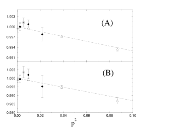
Let us now look at scaling corrections in the one-particle spectrum. In the continuum limit we expect $\omega(\overline{p})\to\sqrt{m^{2}+\overline{p}^{2}}$, and $Z(\overline{p})\to Z$. In Fig. 3.3 we plot the ratios $\omega(\overline{p})/\sqrt{\overline{p}+m^{2}}$ (graph (A)), and $Z(\overline{p})/Z(0)$ (graph (B)). Both this quantities all well described by the same form, see Ref. [83]:

$$\frac{\omega(\overline{p})}{\sqrt{\overline{p}^{2}+m^{2}}} \simeq 1-c_{\omega}\overline{p}^{2}\,,$$ (3.3.19)

$$\frac{Z(\overline{p})}{Z(0)} \simeq 1-c_{Z}\overline{p}^{2}\,.$$ (3.3.20)

The fitting lines in Fig. 3.3 have been obtained using $c_{\omega}=0.07$ and $c_{Z}=0.13$. The fitting form in Eqs. (3.3.19) and (3.3.20) follows from the general behavior of scaling corrections. Let us consider, for instance, the ratio $Z(\overline{p})/Z(0)$. Since the continuum limit of this quantity is equal to one, it behaves as follows:

$$\frac{Z(\overline{p})}{Z(0)}=1+\frac{1}{L^{2}}\Delta_{Z}(mL,\overline{p}L;L)+O(L^{-4})\,,$$ (3.3.21)

with $\Delta_{Z}(\dots;L)$ weakly (logarithmically) depending upon $L$, at $mL$ and $\overline{p}L$ fixed. Since $Z(0)/Z(0)=1$ and $Z(\overline{p})$ is even in $\overline{p}$, it follows that $\Delta_{Z}(mL,\overline{p}L;L)=\Delta^{(1)}_{Z}(mL;L)(\overline{p}L)^{2}+O(\overline{p}^{4})$, whence

$$\frac{Z(\overline{p})}{Z(0)}=1+\Delta^{(1)}_{Z}(mL;L)\overline{p}^{2}+O(\overline{p}^{4})\,,$$ (3.3.22)

which coincides with Eq. (3.3.20). Our three lattices (A), (B) and (C) have approximatively the same physical size $mL$. Because of the logarithmic dependence of $\Delta^{(1)}_{Z}(mL;L)$ upon $L$, the fitting coefficients $c_{\omega}$ and $c_{Z}$ should not be independent of the lattice at $mL$ fixed. However our statistical errors are too large to detect this weak dependence. Finally, let us notice that the behavior described in Eqs. (3.3.19) and (3.3.20) can be recovered in lattice perturbation theory [48]. It is easy to obtain $c_{\omega}=1/12+O(g_{L}^{2})$ (one-loop perturbation theory) and $c_{Z}=1/6+O(g_{L})$ (tree-level perturbation theory). Both these results are in rough agreement with our numerical data. We conclude that for the two largest lattices the spectrum scales at the error-bar level. Instead, for lattice (A) there are tiny (and essentially under control) scaling corrections. These corrections are so small (at most 1%) that we can neglect them in the following discussion.

One can also investigate asymptotic scaling, i.e. the dependence of $\omega(\overline{p})$ and $Z$ on $g_{L}$. The dependence of $\omega(\overline{p})$ can be determined from Eq. (2.8.11). There exists also an exact prediction for $Z$, including the non-perturbative constant [85, 86]. However, as is well known, lattice perturbation theory is not predictive at these values of the correlation length, and indeed, the perturbative four-loop predictions show large discrepancies compared to the numerical data. The agreement is instead quite good [87, 86] if one uses the improved coupling $g_{E}$ defined in Eq. (2.8.7).

	lattice (A)		lattice (B)		lattice (C)
$\overline{p}$	$\omega(\overline{p})$	$Z(\overline{p})$	$\omega(\overline{p})$	$Z(\overline{p})$	$\omega(\overline{p})$	$Z(\overline{p})$
$0$	$0.145393(40)$	$1.6593(8)$	$0.073327(55)$	$1.3563(18)$	$0.036963(34)$	$1.1295(14)$
$2\pi/L$	$0.175380(40)$	$1.6582(8)$	$0.088244(67)$	$1.3557(21)$	$0.044348(35)$	$1.1284(13)$
$4\pi/L$	$0.243657(74)$	$1.6510(13)$	$0.12263(15)$	$1.3591(42)$	$0.061456(66)$	$1.1292(21)$
$6\pi/L$	$0.326327(192)$	$1.6378(32)$	$0.16415(32)$	$1.3499(86)$	$0.082494(109)$	$1.1336(35)$

Table 3.3: The one-particle spectrum and the field normalization for lattices (A), (B), (C).

3.3.3 Non-Perturbative Renormalization of the Lattice Energy-Momentum Tensor

Figure 3.4: Corrections to scaling for the renormalization constant of the energy-momentum tensor, cf. Eq. (3.3.25). The circles correspond the numerical results obtained on lattice (B). The dashed line is the best fitting curve of the form $\zeta(\overline{p})=\widehat{\zeta}_{0}+\widehat{\zeta}_{1}\overline{p}^{2}$.

In this Section we want to compute non-perturbatively the renormalization constant $Z^{L(2,0)}_{TT}$ of the lattice energy-momentum tensor, see Eq. (2.5.1). In general, given an operator $\cal O$ on the lattice, we define its matrix element by

$$\langle\overline{p},a|\hat{\cal O}|\overline{q},b\rangle\equiv N\sqrt{4\omega(\overline{p})\omega(\overline{q})}\lim_{t\to\infty}\widehat{C}^{ab}_{\cal O}(\overline{p},\overline{q};2t).$$ (3.3.23)

For $\overline{\partial}_{\mu}\mbox{\boldmath$\sigma$}\cdot\overline{\partial}_{\nu}\mbox{\boldmath$\sigma$}$ the matrix elements can be obtained from the results given in Tables 3.1 and 3.2. The matrix elements of $(\overline{\partial}_{\mu}\mbox{\boldmath$\sigma$})^{2}$ are dominated by the mixing with the identity operator and thus, in order to define the renormalized operator for $\mu=\nu$, we should perform a non-perturbative subtraction of the large $1/a^{2}$ term, which is practically impossible. Therefore, we only compute the renormalized operator for $\mu\not=\nu$, which amounts to determining the constant $Z^{L,(2,0)}_{TT}$. This constant is obtained by requiring

$$\langle\overline{p},a|T_{01,0}|\overline{p},b\rangle=\,2i\,\overline{p}\sqrt{\overline{p}^{2}+m^{2}}\,\delta^{ab}.$$ (3.3.24)

In practice, we first compute an effective (momentum-dependent) renormalization constant

$$\zeta(\overline{p})\equiv{2\,\overline{p}\,\omega(\overline{p})\,g_{L}\over{\rm Im}\,\langle\overline{p},a|(\overline{\partial}_{0}\mbox{\boldmath$\sigma$}\cdot\overline{\partial}_{1}\mbox{\boldmath$\sigma$})|\overline{p},a\rangle},$$ (3.3.25)

which, in the continuum limit, becomes independent of $\overline{p}$ and converges to $Z^{L(2,0)}_{TT}$. Using the data of Table 3.1, on lattice (B), we obtain $\zeta(\overline{p})=1.040(8)$, $1.048(6)$, $1.059(7)$ for $\overline{p}=2\pi/L$, $4\pi/L$, $6\pi/L$ respectively.

Corrections to scaling are expected to produce the following dependence upon the external momentum: $\zeta(\overline{p})=\zeta_{0}(m)+\zeta_{1}(mL;m)\overline{p}^{2}+O(\overline{p}^{4})$. In Fig. 3.4 we report the numerical results for $\zeta(\overline{p})$, together with the best fitting curve of the form $\zeta(\overline{p})=\widehat{\zeta}_{0}+\widehat{\zeta}_{1}\overline{p}^{2}$. Clearly the scaling corrections are small: we can estimate $Z^{L(2,0)}_{TT}=1.05(2)$ on this lattice. This compares very well with the result of one-loop lattice perturbation theory given in Eq. (2.5.26), which yields $Z^{L(2,0)}_{TT}\simeq 1.044357$, and with the result of “improved” (sometimes called “boosted”) perturbation theory in terms of the coupling $g_{E}$, cf. Eq. (2.8.7), $Z^{L(2,0)}_{TT}=1.052471(3)$ (the error is due to the error on $g_{E}$).

3.3.4 OPE for the Scalar Product of Currents

In this Section we consider the product $j_{0,0}^{ab}j_{1,x}^{ab}$ averaged over rotations. Using Eq. (3.1.1), we have in the continuum scheme

$$\frac{1}{2}\,\overline{j_{0,0}^{ab}j_{1,x}^{ab}}=\left[{1\over 4}W_{2}(r/2)+W_{3}(r/2)+W_{4}(r/2)\right]{1\over g}\left[T_{01}(0)\right]_{\overline{MS}}\,.$$ (3.3.26)

Notice that, since the currents are exactly conserved, both on the lattice and in the continuum, there is no need to make a distinction between lattice and $\overline{\rm MS}$ -renormalized operators. All other contributions vanish after the angular average. Using the results of Sec. 3.1.1 we have at one loop in the $\overline{\rm MS}$ scheme

$$\frac{1}{2}\,\overline{j_{0,0}^{ab}j_{1,x}^{ab}}=\,\left[1-{N-2\over 2\pi}g\left(\log\left({{\mu}r\over 2}\right)+\gamma-{5\over 4}\right)+O(g^{2})\right]{1\over g}\left[T_{01}(0)\right]_{\overline{MS}},$$ (3.3.27)

where $\mu$ is the renormalization scale and $\gamma$ Euler’s constant. We will not use this form of the OPE expansion, but instead the RG-improved Wilson coefficients. Thus, cf. Sec. 2.7, we write

$$\frac{1}{2}\,\overline{j_{0,0}^{ab}j_{1,x}^{ab}}=W_{RGI}(\overline{g}(\Lambda_{\overline{\rm MS}}r))\left[T_{01}(0)\right]_{\overline{MS}},$$ (3.3.28)

where

$$W_{RGI}(\overline{g})=\frac{1}{\overline{g}}\left[1+{5(N-2)\over 8\pi}\overline{g}\right],$$ (3.3.29)

and $\overline{g}(\Lambda_{\overline{\rm MS}}r)$ is the running coupling constant defined by

$$\lambda_{{\overline{\rm MS}}}(\overline{g})=\,\Lambda_{{\overline{\rm MS}}}{re^{\gamma}\over 2}.$$ (3.3.30)

This expression coincides with the one of Sec. 2.7, see Eq. (2.7.12), apart from the factor $e^{\gamma}/2$ which has been inserted for future convenience. Using the perturbative expression (2.7.13), we can also rewrite (3.3.29) as

$$W_{RGI}(r)={N-2\over 2\pi}z+\left[{1\over 2\pi}\log z+\frac{5(N-2)}{8\pi}\right]\,,$$ (3.3.31)

where $z=-\log(\Lambda_{{\overline{\rm MS}}}re^{\gamma}/2)$.

We will also use the lattice Wilson coefficients, see Sec. 3.1.2. Using the one-loop results of Sec. 3.1.2 and the general expressions reported in Sec. 2.7, proceeding as before, we obtain the prediction

$$\frac{1}{2}\,\overline{j_{0,0}^{L,ab}j_{1,x}^{L,ab}}=U(g_{L})W^{L}_{RGI}(\overline{g}_{L}(\Lambda_{L}r))T^{L}_{01,0},$$ (3.3.32)

where, at one loop,

$$W^{L}_{RGI}(\overline{g}_{L}) = \frac{1}{\overline{g}_{L}}\left[1+\left({5N-2\over 8\pi}-\frac{1}{4}\right)\overline{g}_{L}\right],$$ (3.3.33)

$$U(g_{L}) = 1+\left(\frac{1}{\pi}-\frac{1}{4}\right)g_{L},$$ (3.3.34)

and $\overline{g}_{L}(\Lambda_{L}r)$ is the running coupling constant defined by

$$\lambda_{L}(\overline{g}_{L})=\,\Lambda_{L}\,re^{\gamma}\sqrt{8},$$ (3.3.35)

where $\Lambda_{L}$ is the lattice $\Lambda$-parameter, see Sec. 2.7.

Finally we shall test perturbation theory in the “improved” expansion parameter $g_{E}$ defined in Eq. (2.8.7). The OPE becomes:

$$\frac{1}{2}\,\overline{j_{0,0}^{L,ab}j_{1,x}^{L,ab}}=U(g_{E})W^{E}_{RGI}(\overline{g}_{E}(\Lambda_{E}r))T^{L}_{01,0},$$ (3.3.36)

where

$$W^{E}_{RGI}(\overline{g}_{E}) = \frac{1}{\overline{g}_{E}}\left[1+\left({5(N-2)\over 8\pi}-\frac{1}{8}\right)\overline{g}_{E}\right]\ ,$$ (3.3.37)

$U(\cdot)$ is the same as in Eq. (3.3.34), and $\overline{g}_{E}(\Lambda_{E}r)$ is the running coupling constant defined by

$$\lambda_{E}(\overline{g}_{E})=\,\Lambda_{E}\,re^{\gamma}\sqrt{8},$$ (3.3.38)

where $\Lambda_{E}$ is the $\Lambda$-parameter (2.8.9).

We have tested the validity of the OPE by considering matrix elements between one-particle states. The matrix elements of the product of the currents can be determined in terms of $G^{(s)}(t,x;\overline{p},\overline{q};2t_{s})$, since

$$\frac{1}{2}\,\langle\overline{p},c|\mbox{\boldmath$j$}_{0,(0,0)}\cdot\mbox{\boldmath$j$}_{1,(t,x)}|\overline{q},c\rangle=N\sqrt{4\omega(\overline{p})\omega(\overline{q})}\lim_{t_{s}\to\infty}\widehat{G}^{(s)}(t,x;\overline{p},\overline{q};2t_{s}).$$ (3.3.39)

In Fig. 3.5 we report the angular average of ${\rm Im}\ \widehat{G}^{(s)}(t,x;\overline{p},\overline{p};2t_{s})$ for lattices (A) and (B): here $t_{s}=6$, $10$ for the two lattices respectively. In Figs. 3.6, 3.7, and 3.8 we compare these numerical data with the predictions of perturbation theory.

In Fig. 3.6 we use continuum RG-improved perturbation theory in the $\overline{\rm MS}$ scheme. In this case, the matrix element of the energy-momentum tensor is immediately computed: $\langle\overline{p},a|T_{01}|\overline{p},b\rangle=2i\overline{p}\omega(\overline{p})\delta^{ab}$. Therefore, we consider the ratio

$$R(r)=\frac{1}{2}{{\rm Im}\langle\overline{p},c|\overline{\mbox{\boldmath$j$}_{0,(0,0)}\cdot\mbox{\boldmath$j$}_{1,(t,x)}}|\overline{p},c\rangle\over 2\overline{p}\omega(\overline{p})W_{RGI}(\overline{g}(\Lambda_{\overline{\rm MS}}r))},$$ (3.3.40)

which should approach 1 in the short-distance limit. In Fig. 3.6 we present several determinations of $R(r)$ that differ in the way in which the running coupling constant $\overline{g}(\Lambda_{\overline{\rm MS}}r)$ and the $\overline{\rm MS}$ coupling $g$ are determined.

There are several different methods that can be used to compute the $\overline{\rm MS}$ coupling $g$ and the strictly related $\overline{g}(\Lambda_{\overline{\rm MS}}x)$. They have been compared in detail in Sec. 2.8. It turned out that the finite-size scaling method proposed by Lüscher [60, 61] and what we call “the RG-improved perturbative method” are essentially equivalent, see, e.g., Table 2.1. Therefore, we can use either of them, obtaining completely equivalent results. In Fig. 3.6 we have used the finite-size scaling method to be consistent with what we would do in QCD. Elsewhere, we have used the RG improved perturbative method because of its simplicity.

The first step in the computation of $R(r)$ is the determination of $\overline{g}(\Lambda_{\overline{\rm MS}}r)$. This is obtained as follows: we fix $\mu/m$, and using the finite-size scaling results reported in Table 2.1, we compute $g_{\overline{\rm MS}}(\mu)$. Then, using Eq. (2.8.3) we determine $\Lambda_{\overline{\rm MS}}=\mu\lambda_{{\overline{\rm MS}}}(g_{\overline{\rm MS}})$ at $l$-loops. Finally, $\overline{g}(\Lambda_{\overline{\rm MS}}r)$ is obtained either by solving Eq. (3.3.30), again using Eq. (2.8.3) for $\lambda_{\overline{\rm MS}}(\overline{g})$ appearing in the right-hand side, or by using Eq. (2.7.13). As we discussed in Sec. 2.8, the final result should be independent of the chosen value of $\mu/m$ and therefore we can evaluate the systematic error on $\overline{g}(\Lambda_{\overline{\rm MS}}x)$ by considering different values of $\mu/m$. If we fix $m/\mu=0.00071$, cf. first row of Table 2.1, we have $\overline{g}(\Lambda_{\overline{\rm MS}}x)=1.498$, $2.206$, $3.363$ respectively for $mx=0.2$, $0.5$, $0.8$, while if we fix $m/\mu=0.1033$, cf. 10th row of Table 2.1 in App. 2.8, we have $\overline{g}(\Lambda_{\overline{\rm MS}}x)=1.490$, $2.185$, $3.273$ at the same distances. The dependence is tiny and, as expected, it increases for larger values of $mx$. In practice, it does not play any role, the main source of error being instead the truncation of the OPE coefficients. Notice that the independence on $\mu$ is obvious if we use the RG-improved perturbative method.

Let us now describe the various graphs appearing in Fig. 3.6. In graphs (A) and (B) we fix $\mu=m/0.00071$ and then, using the results presented in Table 2.1, cf. first row, we obtain $g_{{\overline{\rm MS}}}(\mu)=0.587016$. We then compute $\Lambda_{{\overline{\rm MS}}}(\mu,g_{{\overline{\rm MS}}})$ using the four-loop expression (2.8.3) with $l=4$. Finally, the Wilson coefficient is given by (3.3.31): in graph (A) we use the leading term only, while in graph (B) we include the next-to-leading one.

In graphs (C) and (D) we compute $\Lambda_{{\overline{\rm MS}}}$ as in (A) and (B), choosing a different scale, $\mu=m/0.1033$, cf. $10^{\rm th}$ row of Table 2.1. Then we compute $\overline{g}(x)$ by solving numerically Eq. (3.3.30) using the four-loop expression (2.8.3) with $l=4$. Finally, the Wilson coefficient is obtained using Eq. (3.3.29). While in graph (C) we keep only the leading term $1/\overline{g}(x)$, in graph (D) we use the complete expression.

Finally, graphs (E) and (F) are identical to graph (D) except that $\Lambda_{{\overline{\rm MS}}}$ and $\overline{g}(x)$ are computed using the two-loop expression (2.8.3) with $l=2$. The two graphs correspond to different choices of $\mu$: $\mu=m/0.00071$ (graph (E)) and $\mu=m/0.1033$ (graph (F)).

Comparing the different graphs, we immediately see that the choice of scale $\mu$ and the order of perturbation theory used for $\Lambda_{\overline{\rm MS}}$ (two loops or four loops) are not relevant with the present statistical errors. Much more important is the role of the Wilson coefficients. If one considers only the leading term (graphs (A) and (C)) there are indeed large discrepancies and in the present case one would obtain estimates of the matrix elements with an error of 50–100%. Inclusion of the next-to-leading term—this amounts to considering one-loop Wilson coefficients and two-loop anomalous dimensions—considerably improves the results, and now the discrepancy is of the order of the statistical errors, approximately 10%. For the practical application of the method, it is important to have criteria for estimating the error on the results. It is evident that the flatness of the ratio of the matrix element by the OPE prediction is not, in this case, a good criterion: The points in graph (A) show a plateau—and for a quite large set of values of $r$—even if the result is wrong by a factor of two. However, this may just be a peculiarity of the case we consider, in which the $r$-dependence of the data and of the OPE coefficients is very weak. On the other hand, the comparison of the results obtained using different methods for determining $\overline{g}(x)$ seems to provide reasonable estimates of the error bars. For instance, if only the leading term of the Wilson coefficients were available, we could have obtained a reasonable estimate of the error by comparing graphs (A) and (C).

In Fig. 3.7 we consider lattice RG-improved perturbation theory, computing

$$R^{\rm latt}(r)=\frac{1}{2}{{\rm Im}\,\langle\overline{p},c|\overline{\mbox{\boldmath$j$}_{0,(0,0)}\cdot\mbox{\boldmath$j$}_{1,(t,x)}}|\overline{p},c\rangle\over U(g_{L})W_{RGI}^{L}(\bar{g}_{L}){\rm Im}\,\langle\overline{p},c|T^{L}_{10}|\overline{p},c\rangle}.$$ (3.3.41)

In graph (A) we use $g_{L}$ as an expansion parameter. We compute $\Lambda_{L}$ using the value of the mass gap $m^{-1}=13.632(6)$ and Eq. (2.8.11), with the non-perturbative constant (2.8.12). Then, we determine $\overline{g}_{L}(\Lambda^{\rm latt}r)$ by solving numerically (3.3.35) and using for $\lambda_{L}(\overline{g}_{L})$ appearing in the left-hand side its truncated four-loop expression (2.8.3). Finally, we use Eq. (3.3.33) for the Wilson coefficient. The results are quite poor: there is a downward trend as a function of $r$ and the data are far too low. Naive lattice perturbation theory is unable to provide a good description of the numerical data.

The results improve significantly if we use the improved coupling $g_{E}$: The estimates obtained using this coupling, graphs (B), (C), (D), are not very different from those obtained using $\overline{\rm MS}$ continuum perturbation theory. Graph (B) has been obtained exactly as graph (A), except that in this case we used $g_{E}$ as an expansion parameter. The $\Lambda$-parameter is defined in (2.8.9), $m/\Lambda_{E}$ in (2.8.10), and the relevant Wilson coefficient is given in Eq. (3.3.37). Graphs (C) and (D) are analogous to graph (B). The difference is in the determination of $\Lambda_{E}$. We do not compute it non-perturbatively by using the mass gap but we determine it directly from the perturbative expression (2.8.9). In this case we use the perturbative expression truncated at four loops (C) and two loops (D).

In Figs. 3.6 and 3.7 we have checked the validity of the OPE on lattice (B). If one has in mind QCD applications this is quite a large lattice since $\xi^{\rm exp}\approx 14$. For this reason, we have tried to understand if the nice agreement we have found survives on a smaller lattice, by repeating the computation on lattice (A). The results are reported in Fig. 3.8. Graphs (A) and (B) should be compared with graph (D) of Fig. 3.6. In (A) we compute $\Lambda_{{\overline{\rm MS}}}$ from Eq. (2.8.1), with the non-perturbative constant (2.8.2) and $m^{-1}=6.878(3)$. Then, we compute $\overline{g}(x)$ solving numerically Eq. (3.3.30) using the four-loop expression (2.8.3) with $l=4$. The Wilson coefficient is obtained from Eq. (3.3.29). In (B) we repeat the same calculation as in Fig. 3.6 graph (D) at the scale $\mu=m/0.00071$. In (C) and (D) we repeat the calculation of graph (B) using the two-loop and the three-loop $\beta$-function for the determination of the coupling $\overline{g}$. In all graphs (B), (C), (D) we use the result $m^{-1}=6.878(3)$.

Graphs (A) and (B) show a nice flat behavior and for $2\mathrel{\hbox to0.0pt{\lower 3.0pt\hbox{$\mathchar 536\relax$}\hss}\raise 2.0pt\hbox{$\mathchar 316\relax$}}r\mathrel{\hbox to0.0pt{\lower 3.0pt\hbox{$\mathchar 536\relax$}\hss}\raise 2.0pt\hbox{$\mathchar 316\relax$}}\xi$, the ratio $R(r)$ is approximately 1 with 2–3% corrections (notice that the vertical scale in Figs. 3.6 and 3.8 is different): The OPE works nicely even on this small lattice. (A) and (B) differ in the method used in the determination of the $\overline{\rm MS}$ coupling. As we explained in App. 2.8 and it appears clearly from the two graphs, the effect is very small. Graph (C)—and to a lesser extent graph (D)—shows instead significant deviations: Clearly, $\overline{g}(\Lambda_{\overline{\rm MS}}x)$ must be determined using four-loop perturbative expansions in order to reduce the systematic error to a few percent. Notice that such discrepancies are probably present also for lattice (B): however, in this case, the statistical errors on $R(r)$ are large—approximately 5-6% (for $\overline{p}=2\pi/L$ and $\overline{p}=4\pi/L$) and 9% (for $\overline{p}=6\pi/L$)—and thus they do not allow to observe this effect.

As a further check we considered matrix elements between states of different momentum. In Fig. 3.9 we report the angular average of ${\rm Im}\ \widehat{G}^{(s)}(t,x;0,\overline{p};20)$ for lattice (B). In Fig. 3.10 we compare the numerical data with the OPE prediction, by considering

$$S(r)=\frac{1}{2}{{\rm Im}\,\langle 0,c|\overline{\mbox{\boldmath$j$}_{0,(0,0)}\cdot\mbox{\boldmath$j$}_{1,(t,x)}}|\overline{p},c\rangle\over W^{RGI}(\bar{g}){\rm Im}\langle 0,c|T_{01}^{\rm latt}|\overline{p},c\rangle},$$ (3.3.42)

where $T_{\mu\nu}^{\rm latt}$ is defined in Eq. (2.5.1) and $Z_{TT}^{L,(2,0)}$ is computed in Sec. 3.3.3. In Fig. 3.10 we report $S(r)$ for lattice (B). The Wilson coefficients are computed as in graph (A) of Fig. 3.8, using $m^{-1}=13.636(10)$. The numerical data are again well described by the OPE prediction for a quite large set of values of $r$.

3.3.5 OPE for the Antisymmetric Product of Currents

In this Section we consider the antisymmetric product of two currents and compare our numerical results with the perturbative predictions. With respect to the previous case, we have here a better knowledge of the perturbative Wilson coefficients—some of them are known to two loops—and moreover we have an exact expression for the one-particle matrix elements of the current $j_{\mu,x}$. Indeed, we have [89, 83]:

$$\langle\overline{p},c|j^{ab}_{\mu,(t,x)}|\overline{q},d\rangle=-i(p_{\mu}+q_{\mu})\,G(k)\,(\delta^{ac}\delta^{bd}-\delta^{ad}\delta^{bc})\,e^{i(p-q)\cdot x},$$ (3.3.43)

where $p\cdot x\equiv p_{0}t+p_{1}x$, $p_{\mu}\equiv(i\sqrt{\overline{p}^{2}+m^{2}},\overline{p})$, $k\equiv\frac{1}{2}\sqrt{(p_{0}-q_{0})^{2}+(p_{1}-q_{1})^{2}}$, and, for $N=3$,

$$G(k)=\frac{\theta}{2\tanh\theta/2}\cdot\frac{\pi^{2}}{\pi^{2}+\theta^{2}},$$ (3.3.44)

where the rapidity variable $\theta$ is defined by $k=m\sinh\theta/2$.

We first consider the product $(j^{ac}_{\mu,(0,0)}j^{bc}_{\nu,(t,x)}-j^{bc}_{\mu,(0,0)}j^{ac}_{\nu,(t,x)})$ for $\mu=\nu=1$ and $x=0$. The OPE of such a product can be determined from Eq. (3.1.16). Using the results of App. 3.2, we have for $t\to 0$,

$$\sum_{c}j^{ac}_{1,(0,0)}j^{bc}_{1,(t,0)}-j^{bc}_{1,(0,0)}j^{ac}_{1,(t,0)}={1\over t}W_{RGI}\left(\overline{g}(\Lambda_{\overline{\rm MS}}t)\right)\left(j_{0}^{ab}(0)+{t\over 2}\partial_{0}j_{0}^{ab}(0)\right),$$ (3.3.45)

where, at two loops,

$$W_{RGI}(\overline{g})={N-2\over 2\pi}+{N-2\over 4\pi^{2}}\overline{g},$$ (3.3.46)

and $\overline{g}(\Lambda_{\overline{\rm MS}}t)$ is defined in Eq. (3.3.30). We also consider the angular average of the product of the currents for $\mu=0$ and $\nu=1$. Using the results of Sec. 3.1.1, we have for $r\to 0$

$$\hskip-28.45274pt{\cal I}^{ab}(r)\equiv\overline{j^{ac}_{0,(0,0)}j^{bc}_{1,(t,x)}-j^{bc}_{0,(0,0)}j^{ac}_{1,(t,x)}}=$$ (3.3.47)

$$\hskip-28.45274pt\qquad-\,{3(N-2)\over 16\pi}\,[\partial_{0}j_{1}^{ab}(0)+\partial_{1}j_{0}^{ab}(0)]+{1\over 2\overline{g}}\left(1+{N-6\over 4\pi}\overline{g}\right)\,[\partial_{0}j_{1}^{ab}(0)-\partial_{1}j_{0}^{ab}(0)]\,.$$

Again, we have tested the validity of the OPE by considering matrix elements between one-particle states. The matrix elements of the product of the currents are obtained from

$$\sum_{abc}\langle\overline{p},a|j^{(ac)}_{(0,0),\mu}j^{(bc)}_{(t,x),\nu}-j^{(bc)}_{(0,0),\mu}j^{(ac)}_{(t,x),\nu}|\overline{q},b\rangle=\,N\sqrt{4\omega(\overline{p})\omega(\overline{q})}\lim_{t_{s}\to\infty}\widehat{G}^{(a)}_{\mu\nu}(t,x;\overline{p},\overline{q};2t_{s}).$$ (3.3.48)

In Fig. 3.11 we show a plot of ${\rm Re}\,\widehat{G}^{(a)}_{11}(t,x;\overline{p},-\overline{p};2t_{s})$ obtained on lattice (B) for $\overline{p}=2\pi/L$ and $t_{s}=10$, and in Fig. 3.12 we show the angular average of ${\rm Im}\,\widehat{G}^{(a)}_{01}(t,x;\overline{p},0;2t_{s})$ on the same lattice and again for $t_{s}=10$. Comparing these graphs with those for the scalar product of the currents, one sees that the matrix elements show here a larger variation with distance, and thus this should provide a stronger test of the validity of the OPE.

In Fig. 3.13 we compare the results for ${\rm Re}\,\widehat{G}^{(a)}_{11}(t,x;\overline{p},-\overline{p};2t_{s})$ with the OPE perturbative predictions. Here, as always in this Section, we use the RG-improved perturbative method to compute $\overline{g}$, using the four-loop expression for the $\beta$ function. As we explained at length in the previous Section, no significant difference is observed if one uses the finite-size scaling method, or improved lattice perturbation theory.

In graphs (A) and (B) we show the combination

$$V(t)\equiv\frac{1}{2}\,\xi^{\rm exp}\,\left[\widehat{G}^{(a)}_{11}(t,0;\overline{p},-\overline{p};2t_{s})-\widehat{G}^{(a)}_{11}(-t,0;\overline{p},-\overline{p};2t_{s})\right]\,,$$ (3.3.49)

for two different values of $\overline{p}$. In the scaling limit $V(t)$ is a function of $\overline{p}\xi^{\rm exp}$ and of $t/\xi^{\rm exp}$. As it can be seen from the graphs our results show a very nice scaling: The data corresponding to the three different lattices clearly fall on a single curve. In the same graphs we also report the OPE prediction (3.3.45), i.e.

$$V^{\rm OPE}(t)\equiv 2N\omega(\overline{p}){\xi^{\rm exp}\over t}W_{RGI}(\overline{g}(\Lambda_{\overline{\rm MS}}t))\langle\overline{p},a|j^{ab}_{0}(0)|-\overline{p},b\rangle.$$ (3.3.50)

Note that $\langle\overline{p},a|\partial_{0}j^{ab}_{0}|-\overline{p},b\rangle=0$, so that the corrections due to higher-order terms in the OPE expansion are of order $t$. In graph (A) and (B) we use only the one-loop Wilson coefficient for $W_{RGI}(\overline{g})$. There is a good agreement between the OPE prediction and the numerical data: quite surprisingly the agreement extends up to 2 lattice spacings.

To better understand the discrepancies, in graphs (C) and (D) we report $V(t)-V^{\rm OPE}(t)$. In graphs (C1) and (C2) we use the one-loop Wilson coefficient, and in (D1) and (D2) the two-loop Wilson coefficient given in Eq. (3.3.46). The numerical data refer to lattice (A) for (C1) and (D1) and to lattice (B) for (C2) and (D2). There is clearly agreement, although here deviations are quantitatively somewhat large, since $V(t)$ is strongly varying. Let us consider for instance the data obtained on lattice (B) for $\overline{p}=2\pi/L$. If we evaluate the matrix element of the Noether current using the numerical estimate of $V(t)$ with $t=3,4,5,6$ we obtain the result with a systematic error of $2\%,14\%,32\%,27\%$ respectively.

In Fig. 3.14 we compare the angular average of ${\rm Im}\,\widehat{G}^{(a)}_{01}(t,x;\overline{p},0;2t_{s})$ (cf. Fig. 3.12) with the OPE prediction, by defining

$$Y(r)={\langle\overline{p},c|{\cal I}^{ab}(r)|0,c\rangle\over\langle\overline{p},c|{\cal I}^{OPE,ab}(r)|0,c\rangle},$$ (3.3.51)

where ${\cal I}^{OPE,ab}(r)$ is the OPE one-loop prediction (3.3.5). Here we use the form-factor prediction (3.3.43) for the matrix elements of the currents, but no significant difference would have been observed if the matrix elements of the currents had been determined numerically. Use of the form-factor prediction allows only a reduction of the statistical errors and thus gives the opportunity for a stronger check of the OPE. Again we observe a nice agreement and a very large window in which the data are well described by perturbative OPE. The systematic error is below the statistical one (which is approximately $10\%$) as soon as $r>2$.

3.4 First Answers

From the examples of short-distance products studied in this Chapter we can draw some first conclusions.

We considered products of the type $j(x)j(0)$. In most of the cases the leading term of the OPE was of order $r^{0}$ (with $r=|x|$), and the first correction, after averaging over rotations, was of order $r^{2}$. In these cases, we can make the following statements, which are valid within the statistical accuracy of our numerical simulations (about $5\div 10\%$, depending upon the particular example):

• We extracted one-particle matrix elements of the type $\langle\overline{p}|j(x)j(0)|\overline{q}\rangle$ from well chosen four-point correlation functions. These correlation functions show a nice scaling behavior as soon as $r\mathrel{\hbox to0.0pt{\lower 3.0pt\hbox{$\mathchar 536\relax$}\hss}\raise 2.0pt\hbox{$\mathchar 318\relax$}}2a$. On general grounds we would expect scaling corrections of order $1/r^{2}$ (among the others). Such scaling corrections cannot be seen in our data. The only relevant lattice artifacts occur at $r\mathrel{\hbox to0.0pt{\lower 3.0pt\hbox{$\mathchar 536\relax$}\hss}\raise 2.0pt\hbox{$\mathchar 316\relax$}}2a$. This is easily understood if we remember that the lattice currents $j^{L,ab}_{\mu,x}$ and $j^{L,cd}_{\nu,0}$ have a spatial extension of one lattice spacing, see Eq. (2.5.36). The lattice artifacts at $r\mathrel{\hbox to0.0pt{\lower 3.0pt\hbox{$\mathchar 536\relax$}\hss}\raise 2.0pt\hbox{$\mathchar 316\relax$}}2a$ are due to contacts between the two operators $j^{L,ab}_{\mu,x}$ and $j^{L,cd}_{\nu,0}$.

  Such a good scaling behavior allows to use the OPE on rather coarse lattices, e.g. on lattice (A) which has a correlation length $\xi^{\exp}=6.878(2)$.

• Power corrections (i.e. terms of order $r^{2}$) are negligible for $r\mathrel{\hbox to0.0pt{\lower 3.0pt\hbox{$\mathchar 536\relax$}\hss}\raise 2.0pt\hbox{$\mathchar 316\relax$}}\xi$. Indeed we did not find evidence for them in our numerical results.

• The running coupling $\overline{g}(\Lambda r)$ can be accurately determined. This determination makes use of the four-loop beta function, and of the lambda parameter. In the $O(N)$ non-linear $\sigma$-model, the lambda parameter can be computed either with the finite-size method, or by using the exact prediction for the mass gap. In QCD there exists no exact prediction fixing the lambda parameter in terms of some low-energy quantity. However, the finite-size method has already given a precise determination of $\Lambda_{QCD}$ for the quenched theory.

  In our case we can compute $\overline{g}(\Lambda r)$ with a few percent accuracy, over all the range $r\mathrel{\hbox to0.0pt{\lower 3.0pt\hbox{$\mathchar 536\relax$}\hss}\raise 2.0pt\hbox{$\mathchar 316\relax$}}\xi$.

• The perturbative computation of the Wilson coefficients seems to be the weakest point of the whole procedure. The use of the leading-log approximation gives grossly inexact (by more than $50\%$) results in most of the cases considered. The next-to-leading-log approximation (which requires the computation of one-loop Wilson coefficients and two-loop anomalous dimensions) yields results with about a $5\%$ accuracy. These statements are valid if a “well-behaved” renormalization scheme (e.g. $\overline{\rm MS}$ ) is adopted. They seem to hold also if improved lattice perturbation theory is used. Naive lattice perturbation theory gives much worser results.

• The use of different resummation methods for the Wilson coefficients seems to give a realistic idea of the systematic error involved in their perturbative calculation.

These conclusions should be perhaps modified if the leading Wilson coefficient has a power-like diverging behavior ($W(r)\sim 1/r$). We studied a single case of this type, see Sec. 3.3.5. In this case we were able to compute the relevant Wilson coefficient up to two-loop order. Nevertheless, the agreement between the OPE prediction and the numerical results was not good as in the other examples.

Figure 3.5: Estimates of $\widehat{G}^{(s)}(t,x;\overline{p},\overline{p};2t_{s})$ averaged over rotations on lattice (A) (upper graph, here $t_{s}=10$) and (B) (lower graph, $t_{s}=6$). Circles, filled squares, and triangles correspond to $\overline{p}=2\pi/L$, $4\pi/L$, and $6\pi/L$ respectively.

Figure 3.6: The scalar product of two Noether currents compared with the OPE prediction: graphs of $R(r)$, cf. (3.3.40), obtained using $\overline{\rm MS}$ RG-improved perturbation theory. Circles, filled squares, and triangles correspond to $\overline{p}=2\pi/L$, $4\pi/L$, and $6\pi/L$ respectively. The data are for lattice (B), $\xi^{\rm exp}=13.636(10)$.

Figure 3.7: The scalar product of two Noether currents compared with the OPE prediction: graphs of $R^{\rm latt}(r)$, cf. (3.3.41), obtained using RG-improved perturbation theory in the coupling $g_{L}$ and in the improved coupling $g_{E}$. Circles, filled squares, and triangles correspond to $\overline{p}=2\pi/L$, $4\pi/L$, and $6\pi/L$ respectively. The data are for lattice (B), $\xi^{\rm exp}=13.636(10)$.

Figure 3.8: The scalar product of two Noether currents compared with the OPE prediction: graphs of $R(r)$, cf. (3.3.40), obtained using $\overline{\rm MS}$ RG-improved perturbation theory. Circles, filled squares, and triangles correspond to $\overline{p}=2\pi/L$, $4\pi/L$, and $6\pi/L$ respectively. The data are for lattice (A), $\xi^{\rm exp}=6.878(3)$. Notice the change of vertical scale compared to Figs. 3.6, 3.7.

Figure 3.9: Estimates of $\widehat{G}^{(s)}(t,x;\overline{p},0;20)$ averaged over rotations on lattice (B). Circles, filled squares, and triangles correspond to $\overline{p}=2\pi/L$, $4\pi/L$, and $6\pi/L$ respectively.

Figure 3.10: The scalar product of two Noether currents compared with the OPE prediction: graphs of $S(r)$, cf. (3.3.42), obtained using $\overline{\rm MS}$ RG-improved perturbation theory. Circles, filled squares, and triangles correspond to $\overline{p}=2\pi/L$, $4\pi/L$, and $6\pi/L$ respectively. The data are for lattice (B), $\xi^{\rm exp}=13.636(10)$.

Figure 3.11: Estimate of $\widehat{G}^{(a)}_{11}(t,x;\overline{p},-\overline{p};20)$ on lattice (B). Here $\overline{p}=2\pi/L$.

Figure 3.12: Angular average of $\widehat{G}^{(a)}_{01}(t,x;\overline{p},0;20)$ on lattice (B). Circles, filled squares, and triangles correspond to $\overline{p}=2\pi/L$, $4\pi/L$, and $6\pi/L$ respectively.

Figure 3.13: Antisymmetric product of two Noether currents for $x=0$ and $t\neq 0$: in graphs (A) and (B) we report estimates of $V(t)$, cf. (3.3.49), and of the OPE prediction $V^{\rm OPE}(t)$, cf. Eq. (3.3.50), The numerical data correspond to $\overline{p}=2\pi/L$ (graph (A)) and $\overline{p}=4\pi/L$ (graph (B)). Stars, diamonds, and circles refer to lattices (A), (B), (C) respectively. In graphs (C) and (D) we show $V(t)-V^{\rm OPE}(t)$. Empty circles refer to $\overline{p}=2\pi/L$ while filled squares to $\overline{p}=4\pi/L$.

Figure 3.14: The antisymmetric product of two Noether currents compared with the OPE prediction: graphs of $Y(r)$, cf. (3.3.51), obtained using $\overline{\rm MS}$ RG-improved perturbation theory. The circles, filled square, and triangles correspond to $\overline{p}=2\pi/L$, $4\pi/L$, and $6\pi/L$ respectively. The data are for lattice (B), $\xi^{\rm exp}=13.636(10)$.

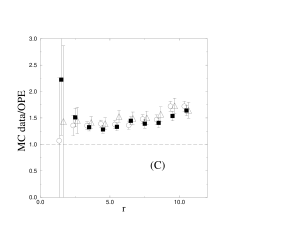
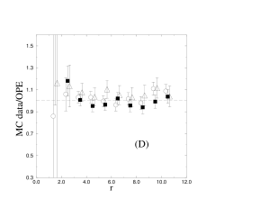
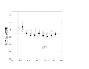
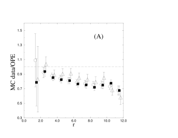
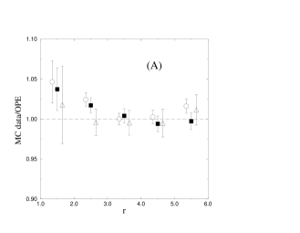
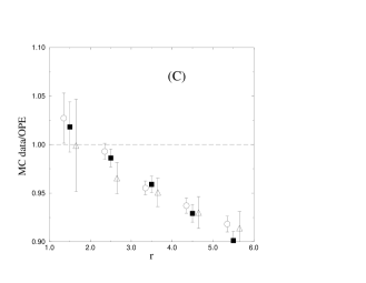
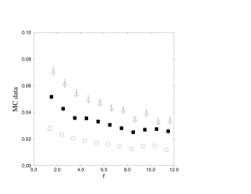
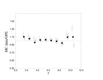
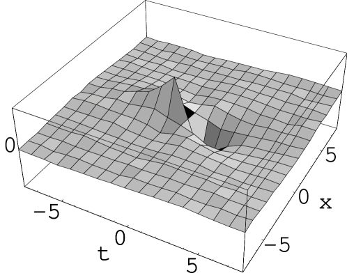
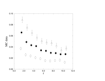
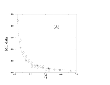
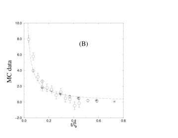
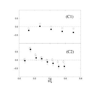
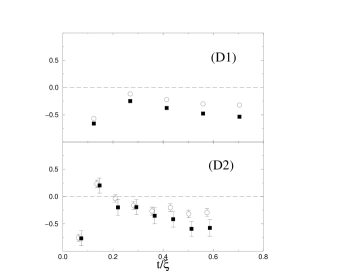
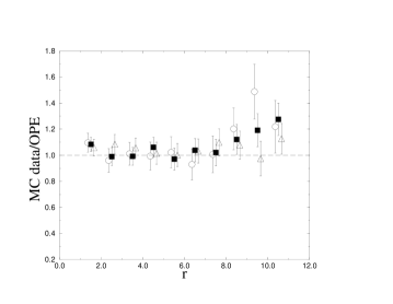
Chapter 4 Operator Product Expansion for Elementary Fields

In this Chapter we shall consider the short-distance expansion of the product of two elementary fields for the $O(N)$ non-linear $\sigma$-model. The motivation for such a study is twofold.

From a numerical point of view, the task is simpler than in the previous Chapter. Computing the product of two fields implies fewer operations than computing the product of two Noether currents. This implies a significative speed up in the algorithms and, as a consequence, much better numerical data. We will be able to discuss finer issues than in the previous Chapter, such as lattice artifacts and next-to-leading terms in the OPE.

Unlike Noether currents, elementary fields require a non-trivial renormalization. This makes the exercise slightly more complicated from a conceptual point of view. We shall be forced to consider the intricacies of renormalization and to compare various (perturbative and non-perturbative) renormalization methods.

As in the previous Chapter, we shall focus on matrix elements between one-particle states. Generally speaking, we shall consider the following OPE:

$$\langle\overline{p}|\sigma(x)\sigma(-x)|\overline{p}\rangle\sim W_{\cal O}(x)\langle\overline{p}|{\cal O}|\overline{p}\rangle+\sum_{\cal Q}W_{\cal Q}(x)\langle\overline{p}|{\cal Q}|\overline{p}\rangle\,,$$ (4.0.1)

where, once more, we neglected $O(N)$ indices. They will be specified in Sec. 4.4. In the above equation ${\cal O}$ is the leading term of the OPE. The corresponding Wilson coefficient $W_{\cal O}(x)$ is of order $r^{0}$ or $r$ (we recall that $r=|x|$), depending upon the specific example. In the cases we considered, ${\cal O}$ does not mix with any other operator (it renormalizes multiplicatively). The other terms, denoted generically as ${\cal Q}$, are power corrections of relative order $r^{2}$. The operators ${\cal Q}$ have a non-trivial mixing structure.

We evaluated the left-hand side of Eq. (4.0.1) in lattice simulations for $r\mathrel{\hbox to0.0pt{\lower 3.0pt\hbox{$\mathchar 536\relax$}\hss}\raise 2.0pt\hbox{$\mathchar 316\relax$}}\xi$. Notice that the separation between the two field operators on the left-hand side of Eq. (4.0.1) is $2x$. This means that, in this Chapter, we are probing larger distances than in the previous one. We expect that power corrections, i.e. the ${\cal Q}$ terms in Eq. (4.0.1), will not be negligible on such distances.

In this Chapter we mimic what would be done in a physical (QCD) application of the OPE method. We fit the numerical results for the l.h.s. of Eq. (4.0.1), using the r.h.s. as fitting form, and keep the matrix elements $\langle\overline{p}|{\cal O}|\overline{p}\rangle$ and $\langle\overline{p}|{\cal Q}|\overline{p}\rangle$ as fitting parameters. Finally we compare the results for $\langle\overline{p}|{\cal O}|\overline{p}\rangle$ with some independent prediction, either numerical or analytical, for the same quantity.

We restrict the fit to the window $\rho\leq|x|\leq R$, and study the dependence of the results upon the window. In particular we shall focus on the outer limit $R$. We learned in the previous Chapter that the principal source of error, in comparing the OPE with lattice simulations, is the perturbative truncation of the Wilson coefficients. This systematic error depends upon $R$, and in particular vanishes as $R/\xi\to 0$ because of asymptotic freedom. The crucial point is that we cannot easily take the limit $R/\xi\to 0$ because of lattice artifacts (which force us to consider $R\gg 1$) and of finite-size effects (for avoiding them, we must take $\xi\ll L$, $L$ being the linear size of the lattice).

We shall also consider the evaluation of the matrix elements $\langle\overline{p}|{\cal Q}|\overline{p}\rangle$ of the non-leading operators in the OPE. It turns out that a distinction must be made among these operators. Those which do not mix with the leading one (${\cal O}$) can be fixed through Eq. (4.0.1), adopting a perturbative determination of the Wilson coefficients. Nevertheless the computation is, in practice, quite difficult. The determination of the other operators, those that mix with ${\cal O}$, is instead impossible, even from a theoretical point of view. Such a calculation would require a non-perturbative knowledge of the leading Wilson coefficient $W_{\cal O}(x)$.

This Chapter is organized as follows. In Sec. 4.1 we recall some well-known properties of perturbative expansions in quantum field theory. We discuss the consequences of these properties on our non-perturbative renormalization method. In Sec. 4.2 we write the structure of the OPE for two elementary fields, including $O(r^{2})$ terms, and we list the perturbative results for the Wilson coefficients. In Sec. 4.3 we show how to solve the RG equation if a resonance occurs in the anomalous dimensions matrix, cf Sec. 2.7. In Sec. 4.4 we explain the details of the fitting procedure, and we present our numerical results. Finally we summarize our conclusions in Sec. 4.5.

4.1 Perturbative Expansions and OPE

As we explained above, in this Chapter we shall keep track of the next-to-leading terms in the OPE. Our interest is twofold. First of all this may improve the determination of the leading operator. Moreover we want to understand if it is possible to estimate next-to-leading operators.

It turns out that there is some theoretical difficulty in estimating next-to-leading operators in the OPE when they mix with the leading one. This theoretical difficulties are related to the diseases of perturbative expansions, namely to renormalons. In this Section we try to describe these difficulties.

The Section is divided in two parts. In the first one we review some well-known facts concerning the perturbative series of renormalizable asymptotically-free theories. The intent is mainly pedagogical. Rather than making general statements, we look at simple examples taken from the $O(N)$ non-linear $\sigma$-model at large $N$. This has been an important toy model for the study of such problems. For a complete review on renormalons we refer to [90]. In the second part of this Section we discuss the possibility of evaluating the matrix elements of next-to-leading operators which mix with the leading one.

4.1.1 The Limits of Perturbative Expansions

For our discussion it is convenient to introduce the widespread language of Borel transforms. Perturbation theory yields physical quantities in the form of asymptotic series:

$$F(g)\sim\sum_{n=0}^{\infty}F_{n}g^{n}\,.$$ (4.1.1)

In order to recover $F(g)$ from the r.h.s. of Eq. (4.1.1) one needs, in general, additional informations beyond (all) the coefficients $F_{n}$. These informations usually concern the analyticity properties of $F(g)$. A simple example is the case in which $F(g)$ is analytic in a neighborhood of $g=0$. Then, $F(g)$ is obtained by summing the r.h.s. of Eq. (4.1.1) for $|g|$ smaller than the convergence radius and by analytic continuation outside.

Unfortunately this case is not realized in any non-trivial field-theoretical example.

The next simpler situation is realized in several interesting cases (e.g. $\phi^{4}_{d}$ theory with $d<4$) and is described by the hypothesis of the Nevalinna-Sokal theorem [91]:

• $F(g)$ is analytic inside a disc ${\cal K}(\rho)$ of radius $\rho>0$ and center $g_{0}$ with ${\rm Re}(g_{0})=\rho$ and ${\rm Im}(g_{0})=0$.

• The remainder $R_{M}(g)\equiv F(g)-\sum_{n=0}^{M-1}F_{n}g^{n}$ satisfies the bound

  $$|R_{M}(g)|<A\mu^{M}M!|g|^{M}\quad\quad\forall\quad g\in{\cal K}(\rho)\,.$$ (4.1.2)

When the previous hypothesis are realized, the function $F(g)$ is uniquely determined by the coefficients $F_{n}$ through the following construction. One defines the Borel transform of the series (4.1.1) as the formal series given below

$$F_{\cal B}(z)\sim\sum_{n=0}^{\infty}\frac{F_{n}}{n!}z^{n}\,.$$ (4.1.3)

Under the hypotheses I and II it can be proved that the sum on the r.h.s. of Eq. (4.1.3) converges for $|z|<\delta$, $\delta>0$. We can promote $F_{\cal B}(z)$ to the status of an analytic function. Moreover it can be proved that $F_{\cal B}(z)$ is analytic inside the strip $\{{\rm Im}(z)<\delta^{\prime},{\rm Re}(z)>0\}$ and that the integral

$${\widetilde{F}}(g)\equiv\frac{1}{g}\int_{0}^{\infty}\!dz\,F_{\cal B}(z)\,e^{-z/g}$$ (4.1.4)

is finite and equal to $F(g)$ for $g\in{\cal K}(\rho)$.

The physically interesting case of four-dimensional non-abelian gauge theories does not fit in the above picture. In this case there is no exact result about the properties of perturbative expansions. Here we recall the standard picture, which is based on heuristic calculations. The large-order behavior of the perturbative coefficients is $F_{n}\sim\mbox{const.}(\beta_{0}/2)^{n}\Gamma(n+1+2\beta_{1}/\beta_{0}^{2})$, where $-\beta_{0}$ and $-\beta_{1}$ are the first two coefficients of the beta-function, see Eq. (2.1.10). This behaviour is compatible with the hypothesis II. However, the analiticity region of $F(g)$ is a wedge of zero opening angle with the tip at the origin. The essential ingredients for the above picture are renormalizability and asymptotic freedom. As a consequence similar statements hold for the two-dimensional $O(N)$ non-linear $\sigma$-model.

In order to study the concepts outlined above in a simple model we shall consider the $O(N)$ nonlinear $\sigma$-model in the limit $N\to\infty$. In this Section we fix the field and coupling-constant renormalizations by requiring:

$$\Gamma^{(2)}(p)_{ab}=Z^{-1}\left[m^{2}+p^{2}+O(p^{4})\right]\,\delta^{ab}\equiv Z^{-1}\Gamma_{R}^{(2)}(p)_{ab}\,,$$ (4.1.5)

where $\Gamma^{(2)}(p)_{ab}$ is the two-point vertex function. It is moreover convenient to define the running coupling at the scale $\mu^{2}$ by using the renormalization-group equation $\mu\frac{\partial g(\mu)}{\partial\mu}=\beta(g(\mu))$. At leading order in $1/N$, $\beta(g)=-g^{2}/2\pi$, whence

$$g(\mu)=\frac{4\pi}{\log\mu^{2}/m^{2}}+O(1/N)\,.$$ (4.1.6)

We start with a simple example of physical observable, and consider its perturbative expansion. We define the effective coupling $\hat{g}(p)$ as follows in terms of the four-point vertex function $\Gamma^{(4)}(p_{1},p_{2},p_{3},p_{4})_{abcd}$  :

$$\Gamma^{(4)}(p_{1},p_{2},p_{3},p_{4})_{abcd} = \delta^{ab}\delta^{cd}\Gamma(p_{1},p_{2}|p_{3},p_{4})+\delta^{ac}\delta^{bd}\Gamma(p_{1},p_{3}|p_{2},p_{4})+$$

$$+\delta^{ad}\delta^{bc}\Gamma(p_{1},p_{4}|p_{2},p_{3})\,,$$

$$\Gamma(p/2,p/2|-p/2,-p/2) \equiv -Z^{-2}\frac{\hat{g}(p)}{N}(p^{2}+m^{2})\,.$$ (4.1.7)

Being a renormalization group invariant quantity, $\hat{g}(p)$ will be a function of $p^{2}/m^{2}$. It can be rewritten as a function of the the running coupling $g(p)$ at the scale $p^{2}$, see Eq. (4.1.6). The leading term in the $1/N$ expansion of $\hat{g}(p)$ is given by

$$\hat{g}(p)=4\pi\frac{\sqrt{1+4e^{-4\pi/g(p)}}}{1+e^{-4\pi/g(p)}}\left\{\log\left[\frac{\sqrt{1+4e^{-4\pi/g(p)}}+1}{\sqrt{1+4e^{-4\pi/g(p)}}-1}\right]\right\}^{-1}+O(1/N)\,.$$ (4.1.8)

Let us make a few observation concerning this very simple result:

1. For small positive $g(p)$ we have $\hat{g}=g+(g-g^{2}/2\pi)e^{-4\pi/g}+O(e^{-8\pi/g})$. The “perturbative” part of this expansion is trivial; it is obviously analytic in the whole complex plane. Nevertheless it does not determine $\hat{g}(p)$ uniquely. The next terms are of order $e^{-4\pi/g(p)}=m^{2}/p^{2}$. These are the so-called “power corrections”.

2. The singularity structure of $\hat{g}(p)$ is nontrivial, including:

   1. Simple poles at $\frac{4\pi}{g}=(2n+1)i\pi$ with $n\in\mathbb{Z}$. These poles are of “kinematical” origin: they appear because we factored out the term $(p^{2}+m^{2})$ in the definition (4.1.1) of $\hat{g}(p)$.

   2. Branching points at $\frac{4\pi}{g}=\log 4+(2n+1)i\pi$, $n\in\mathbb{Z}$. These singularities were predicted on general grounds by ’t Hooft in Ref. [92]. They are the traces of the two-particle threshold at $p^{2}=-4m^{2}$.

3. The function on the r.h.s. of Eq. (4.1.8) does not satisfies the hypotheses of the Nevalinna-Sokal theorem. If they were satisfied, we could sum the perturbative series using the Borel procedure obtaining the wrong result $\hat{g}(p)=g(p)$. Indeed, although the function is analytic in any disc ${\cal K}(\rho)$ with $\rho<4\pi/\log 4$, it does not satisfy the bound in Eq. (4.1.2) for any $M\geq 1$. In fact, for $M>1$, we get $R_{M}(g)=\hat{g}(g)-g$ and we remark that $\hat{g}(g)$ is periodic along the circles $1/g=1/g_{0}+i\theta$ with $-\infty<\theta<+\infty$ These circles pass through the origin $g=0$ and belong to the disc ${\cal K}(\rho)$ for $g_{0}<\rho$. Therefore, we can approach the origin through one of these circles. The bound (4.1.2) is violated because of the periodicity of $\hat{g}(g)$.

Let us now consider a less straightforward computation. The self-energy is defined as follows:

$$\Gamma^{(2)}_{R}(p;m^{2})\equiv p^{2}+m^{2}+\frac{1}{N}\Sigma(p;m^{2})\,.$$ (4.1.9)

The leading term in the $1/N$ expansion of $\Sigma(p;m^{2})$ is given by

$$\Sigma(p;m^{2})=\int\frac{d^{2}q}{(2\pi)^{2}}\left[\frac{q^{2}+m^{2}}{(p+q)^{2}+m^{2}}\right]_{(2)}\hat{g}(q)+O(1/N)\,,$$ (4.1.10)

where $[F(p,q)]_{(n)}$ denotes zero momentum subtraction up to the $n^{\rm th}$ order in the external momentum $p$. The integral in Eq. (4.1.10) has been considered in Ref. [93]. One obtains, as a byproduct of its computation, the whole perturbative series for $\Sigma(p;m^{2})$ which reads:

$$\Sigma(p;m^{2}) \sim p^{2}\left\{\log\frac{g(p)}{4\pi}+{\rm const.}-\frac{g(p)}{2\pi}+\right.$$

$$\phantom{p^{2}\left\{\right.}\left.+\sum_{n=1}^{\infty}n!\left[(1+(-1)^{n})\,\zeta(n+1)-2\right]\left(\frac{g(p)}{4\pi}\right)^{n+1}\right\}\,,$$

where $\zeta(z)\equiv\sum_{k=1}^{\infty}k^{-z}$ is the Riemann zeta function. Let us quote some simple remarks:

1. The series on the r.h.s. of Eq. (4.1.1) has zero radius of convergence. The coefficients have the general large order behavior $\Sigma_{n}\sim{\rm const.}\,[1-(-1)^{n}](\beta_{0}/2)^{n}\Gamma(n+1)$.

2. The function $\Sigma(p;m^{2})$ does not satisfy the hypothesis of the Nevalinna-Sokal theorem. If they were satisfied the Borel transform of the series in Eq. (4.1.1) would be analytic on the real axis. Indeed we obtain (neglecting the $\log g(p)/4\pi$ and the constant):

   $$\Sigma^{\rm pert}_{\cal B}(z)=-\frac{p^{2}}{4\pi}\left[\frac{2}{1-z/4\pi}+\psi(1+z/4\pi)+\psi(1-z/4\pi)+2\gamma\right\}\,,$$ (4.1.12)

   which has simple poles at $z=4n\pi$ with $n\in\mathbb{Z}$, $n\neq 0$. Singularities occurring within this pattern are usually denoted as “renormalons”.

3. One can “resum” the series (4.1.1) through the integral (4.1.4) by assigning a prescription on each singularities of $\Sigma^{\rm pert}_{\cal B}(z)$. Examples of such prescriptions are: take the Cauchy principal value at each pole; move slightly upward (downward) in the complex planes all the poles; move the pole at $z=4n\pi$ to $z_{\epsilon}=4n\pi+i(-1)^{n}\epsilon$, and so on. Notice that, since the first pole is at $z=4\pi$ these prescriptions yield resummations which differ by terms of relative order $\exp(-4\pi/g(p))=m^{2}/p^{2}$.

The last of these observations is often rephrased by saying that the perturbative expansion fixes physical quantities up to an ambiguity of order $m^{2}/p^{2}$. This is the “standard wisdom” on the problem and is by no means self-evident. Indeed we could add to a given resummation a term of the type $\exp(-4\pi t/g(p))=(m^{2}/p^{2})^{t}$ without modifying its asymptotic expansion.

However it is commonly believed that the correct physical quantity can be recovered by assigning a prescription at the renormalon singularities. We could associate to any perturbative expansion a family of “minimally ambiguous” resummations, each one corresponding to a well-defined prescription at renormalon singularities. Any two of these resummed expansions differ by terms of order $m^{2}/p^{2}$. The correct resummation lies among them but, in order to recover it, some non-perturbative input is required.

4.1.2 The Definition of Composite Operators

Let us now consider a simple example of OPE:

$${\cal A}(x){\cal B}(-x)\sim W_{\cal O}(r){\cal O}+W_{\cal Q}(r)r^{2}{\cal Q}+O(r^{4})\,.$$ (4.1.13)

For sake of simplicity we considered the Wilson coefficients to be rotationally invariant, i.e. to depend upon $x$ uniquely through its modulus $r$. Such a behavior can be enforced by averaging over rotations. Moreover we made explicit the power-like $r$ dependence of the Wilson coefficients. Both $W_{\cal O}(r)$ and $W_{\cal Q}(r)$ are of order $r^{0}$. Finally let ${\cal O}$ and ${\cal Q}$ have the same (internal and Lorentz) symmetries. As a consequence they will mix under renormalization.

We suppose the renormalized operators ${\cal A}$ and ${\cal B}$ on the l.h.s. of Eq. (4.1.13) to be non-perturbatively known. Hereafter we shall focus on the RGI operators ${\cal A}_{RGI}$, ${\cal B}_{RGI}$, ${\cal O}_{RGI}$, ${\cal Q}_{RGI}$, and the corresponding Wilson coefficients $W_{{\cal O},RGI}$, $W_{{\cal Q},RGI}$. With a slight abuse of notation we shall drop the subscripts $RGI$ in this Subsection.

As usual, everything we know about the Wilson coefficients $W_{\cal O}(r)$ ($W_{\cal Q}(r)$) is their $l$-loop (respectively, $m$-loop) perturbative expansions. If we resum the perturbative series using the renormalization group, see Sec. 2.7, we obtain:

$$W^{(l)}_{\cal O}(r)=\overline{g}(r)^{\Gamma_{\cal O}}\sum_{k=0}^{l}W_{{\cal O},k}\,\overline{g}(r)^{k}\,,$$ (4.1.14)

and an analogous formula for $W^{(m)}_{\cal Q}(x)$.

Notice that Eq. (4.1.13) allows to define the composite operator ${\cal O}$ regardless of the precise value of $l\geq 0$:

$${\cal O}(x)\equiv\lim_{\eta\to 0}\frac{{\cal A}(x+\eta){\cal B}(x-\eta)}{W^{(l)}_{\cal O}(|\eta|)}\,.$$ (4.1.15)

Both the left-hand and right-hand sides of the above equation must be interpreted as inserted in a correlation function. This correlation function must be taken with elementary fields $\sigma^{a_{1}}(y_{1}),\dots,\sigma^{a_{n}}(y_{n})$ at space-time points $y_{i}$ distinct from $x$: $\langle(\,\cdot\,)\,\sigma^{a_{1}}(y_{1})\dots\sigma^{a_{n}}(y_{n})\rangle$ ($y_{i}\neq x$). Apart from this specification Eq. (4.1.15) is an exact definition because of asymptotic freedom. The $\eta\to 0$ limit is approached with corrections of relative order $|\log\Lambda\eta|^{-l-1}$. Equation (4.1.15) is the theoretical basis of the non-perturbative renormalization method studied in this thesis.

Let us now take a step further and see whether Eq. (4.1.13) can be used to define the next-lo-leading operator ${\cal Q}$. The naive approach would be to fix ${\cal O}$ from Eq. (4.1.15), and then subtract its contribution from the OPE (4.1.13). In other words one would define ${\cal Q}$ through the following short distance limit:

$$\lim_{\eta\to 0}\frac{{\cal A}(x+\eta){\cal B}(x-\eta)-W^{(l)}_{\cal O}(|\eta|){\cal O}(x)}{\eta^{2}W^{(m)}_{\cal Q}(|\eta|)}\,.$$ (4.1.16)

This procedure is equivalent to using Eq. (4.1.13) as a fitting form, restricting the fit to the window $\rho\leq r\leq R$ and considering the $1\ll\rho,R\ll\xi$ regime. This is what we do in Sec. 4.4.

The problem with Eq. (4.1.16) is evident: the $\eta\to 0$ limit diverges. The $\eta\to 0$ behavior of the ratio in Eq. (4.1.16) is easily obtained using Eq. (4.1.13):

$$\frac{W_{\cal O}(|\eta|)-W^{(l)}_{\cal O}(|\eta|)}{\eta^{2}W^{(m)}_{\cal Q}(|\eta|)}{\cal O}(x)\sim|\log\Lambda\eta|^{\widehat{\Gamma}}\eta^{-2}{\cal O}(x)\,.$$ (4.1.17)

where $\widehat{\Gamma}=\Gamma_{\cal O}-\Gamma_{\cal Q}-l-1$.

The problem we encountered do not disappear if we push the perturbative calculation of Wilson coefficients to high orders. Let us suppose, for instance, that we know the coefficients $W_{{\cal O},k}$ for any $k$, see Eq. (4.1.14). The series (4.1.14) with $l=\infty$ will diverge, as explained in Sec. 4.1.1. Nevertheless we can try to sum it, i.e. to find a function $W^{(\infty)}_{\cal O}(\overline{g}(r))$ whose asymptotic expansion for $\overline{g}\to 0$ coincides with the perturbative one. We can moreover require $W^{(\infty)}_{\cal O}(\overline{g}(r))$ to have the minimum possible ambiguity. This prescription should be understood in the sense explained in the previous Subsection.

Even if we have such a minimally ambiguous Wilson coefficient $W^{(\infty)}_{\cal O}(\overline{g}(r))$, we are left with a great freedom. This freedom correspond to the choice of the prescription at the renormalon singularities. It produces an ambiguity of order $\Lambda^{2}r^{2}$.

Let us now repeat the construction outlined in Eq. (4.1.16) using the new Wilson coefficient $W^{(\infty)}_{\cal O}(\overline{g}(r))$. We get:

$$\frac{{\cal A}(x+\eta){\cal B}(x-\eta)-W^{(\infty)}_{\cal O}(|\eta|){\cal O}(x)}{\eta^{2}W^{(m)}_{\cal Q}(|\eta|)}\approx\frac{W_{\cal O}(|\eta|)-W^{(\infty)}_{\cal O}(|\eta|)}{\eta^{2}W^{(m)}_{\cal Q}(|\eta|)}{\cal O}(x)+\frac{W_{\cal Q}(|\eta|)}{W^{(m)}_{\cal Q}(|\eta|)}{\cal Q}(x)\,.$$

(4.1.18)

According to a conjecture due to Parisi [94, 95, 96], the ambiguities in the perturbative series are strictly related to the power corrections in the OPE. In our case we get:

$$W^{(\infty)}_{\cal O}(r)-W_{\cal O}(r)={\rm const.}\,(\Lambda r)^{2}|\log\Lambda r|^{-\Gamma_{\cal Q}}[1+O(|\log\Lambda r|^{-1})]\,.$$ (4.1.19)

Using this formula we can further elaborate Eq. (4.1.18), obtaining

$$\lim_{\eta\to 0}\frac{{\cal A}(x+\eta){\cal B}(x-\eta)-W^{(\infty)}_{\cal O}(|\eta|){\cal O}(x)}{\eta^{2}W^{(m)}_{\cal Q}(|\eta|)}={\cal Q}(x)+{\rm const.}\,{\cal O}(x)\,.$$ (4.1.20)

Even if we know the whole perturbative series for the leading Wilson coefficient, we cannot fix the next-to-leading operator from the OPE (4.1.13). The renormalon ambiguity in the leading Wilson coefficient is accompanied by the ambiguity of the additive renormalization of the next-to-leading operator. David [97, 98, 99] studied this phenomenon in the $O(N)$ nonlinear $\sigma$-model at large $N$.

Our discussion does not exclude the possibility of estimating the next-to-leading operator ${\cal Q}$ from the OPE (4.1.13). Nevertheless such a calculation cannot be accomplished by naively substituting the coefficients $W_{\cal O}(x)$ and $W_{\cal Q}(x)$ by their perturbative truncation. A clever and accurate definition of the Wilson coefficients is required. This definition should be matched with the appropriate definition for the composite operator ${\cal Q}$.

4.2 Perturbative Calculation of the Wilson Coefficients

In order to apply the OPE renormalization method, we have to compute the OPE of two elementary fields in perturbation theory.

The product of two fields can be decomposed in terms of irreducible representations of $O(N)$. We get a scalar, an antisymmetric rank-2 tensor, and a symmetric traceless rank-2 tensor:

$$\sigma^{a}(x)\sigma^{b}(-x) = \frac{\delta^{ab}}{N}\mbox{\boldmath$\sigma$}(x)\cdot\mbox{\boldmath$\sigma$}(-x)+\frac{1}{2}\left[\sigma^{a}(x)\sigma^{b}(-x)-\sigma^{b}(x)\sigma^{a}(-x)\right]+$$ (4.2.1)

$$+\frac{1}{2}\left[\sigma^{a}(x)\sigma^{b}(-x)+\sigma^{b}(x)\sigma^{a}(-x)-\frac{2\delta^{ab}}{N}\mbox{\boldmath$\sigma$}(x)\cdot\mbox{\boldmath$\sigma$}(-x)\right]\,.$$

It is convenient to introduce the following notation for the symmetrized and antisymmetrized products: $\sigma^{[a}(x)\sigma^{b]}(y)=\sigma^{a}(x)\sigma^{b}(y)-\sigma^{b}(x)\sigma^{a}(y)$, and $\sigma^{\{a}(x)\sigma^{b\}}(y)=\sigma^{a}(x)\sigma^{b}(y)+\sigma^{b}(x)\sigma^{a}(y)$. As we explained in the previous Chapter, the form of OPE is dictated by $O(N)$ symmetry and Lorentz invariance. Let us write it explicitly up to $O(x^{2})$ terms:

$$\mbox{\boldmath$\sigma$}(x)\cdot\mbox{\boldmath$\sigma$}(-x) = F^{(0)}_{0}(x)\mbox{\boldmath$1$}+F^{(0)}_{1}(x)T_{\mu\rho}+$$ (4.2.2)

$$+F^{(0)}_{2}(x)\left[(\partial\mbox{\boldmath$\sigma$})^{2}\right]_{\overline{MS}}+F^{(0)}_{3}(x)\left[\alpha\right]_{\overline{MS}}+O(x^{4})\,,$$

$$\sigma^{[a}(x)\sigma^{b]}(-x) = 2gF^{(1)}_{0}(x)\,j^{ab}_{\mu}+O(x^{3})\,,$$ (4.2.3)

$$\frac{1}{2}\sigma^{\{a}(x)\sigma^{b\}}(-x)-\hskip 56.9055pt$$ (4.2.4)

$$-\frac{\delta^{ab}}{N}\mbox{\boldmath$\sigma$}(x)\cdot\mbox{\boldmath$\sigma$}(-x) = F^{(2)}_{0}(x)\left[S_{0}\right]_{\overline{MS}}+\sum_{k=1}^{7}F^{(2)}_{k}(x)\left[S_{k}\right]_{\overline{MS}}+O(x^{4})\,,$$

where we defined

$$S^{ab}_{0}\equiv\sigma^{a}\sigma^{b}-\frac{1}{Z}\frac{\delta^{ab}}{N}\,.$$ (4.2.5)

The symmmetric traceless dimension 2 operators $S_{1},\dots,S_{7}$ are defined in Eqs. (2.3.24)–(2.3.30). All the operators on the right-hand sides of Eqs. (4.2.2)–(4.2.4) are understood at the space-time position $x=0$. For sake of simplicity we dropped the Lorentz indices of the Wilson coefficients in Eqs. (4.2.2)–(4.2.4). In Eq. (4.2.4) we neglected the Lorentz indices also on the operators $S_{1}$, $S_{2}$ and $S_{5}$. The indices can be restored without ambiguity. Summation over repeated indices is understood.

The Wilson coefficients $F^{(n)}_{i}(x)=F^{(n)}_{i}(x;\mu,g)$ can be computed in perturbation theory. We computed the leading coefficient $F^{(n)}_{0}$ at two-loop order, and the next-to-leading coefficients $F_{i}^{(n)}$, $i\geq 1$ at one-loop order. Using the results for the anomalous dimensions given in Sec. 2.4, we are able to resum the $F^{(n)}_{0}$ at next-to-next-to-leading log, and the $F^{(n)}_{i}$, $i\geq 1$ at next-to-leading log order. The outcomes of the resummation procedure are given in Secs. 4.3 and 4.4.

Let us begin from the scalar sector, see Eq. (4.2.2). In this case the leading Wilson coefficient is known at three-loop order [100, 101]. Since the field anomalous dimensions are known at four-loop order [43, 44], see Sec. 2.1, we can resum this coefficient at (next-to-)³leading log order, cf. Eq. (4.4.24). For greater convenience of the reader, we give below a complete list of the perturbative results:

$$F^{(0)}_{0}(x;\mu,g) = 1-\frac{N-1}{2\pi}g\left(\gamma+\log\mu r\right)+\frac{N-1}{8\pi^{2}}g^{2}\left(\gamma+\log\mu r\right)^{2}+$$

$$+g^{3}\left\{\frac{(N-1)(N-3)}{48\pi^{3}}(\gamma+\log\mu r)^{3}-\frac{(N-1)(N-2)}{16\pi^{3}}(\gamma+\log\mu r)^{2}-\right.$$

$$\left.-\frac{3(N-1)(N-2)}{32\pi^{3}}(\gamma+\log\mu r)+\frac{(N-1)(N-2)}{32\pi^{3}}\left(\zeta(3)-\frac{3}{2}\right)\right\}+O(g^{4})\,,$$

$$F^{(0)}_{1}(x;\mu,g) = -2gx_{\mu}x_{\rho}\left[1-\frac{1}{2\pi}g(\gamma+\log\mu r)+O(g^{2})\right]\,,$$ (4.2.7)

$$F^{(0)}_{2}(x;\mu,g) = -x^{2}\left[1-\frac{1}{4\pi}g+O(g^{2})\right]\,,$$ (4.2.8)

$$F^{(0)}_{3}(x;\mu,g) = x^{2}\left[-\frac{N-1}{2\pi}g\left(\gamma+\log\mu r-\frac{1}{2}\right)+O(g^{2})\right]\,.$$ (4.2.9)

Next we consider the antisymmetric sector, see Eq. (4.2.3). Here we limit ourselves to the leading term of the OPE:

$$F^{(1)}_{0}(x;\mu,g) = -x_{\mu}\left[1-\frac{1}{2\pi}g(\gamma+\log\mu r)-\frac{N-3}{8\pi^{2}}g^{2}(\gamma+\log\mu r)^{2}+\right.$$

$$\phantom{2x_{\mu}\left[\right.}\left.+\frac{N-2}{4\pi^{2}}g^{2}(\gamma+\log\mu r)-\frac{N-2}{16\pi^{2}}g^{2}+O(g^{3})\right]\,.$$

In Sec. 4.4.8 we shall also consider the power corrections (of relative order $r^{2}$) to this leading behavior. Since we did not compute them in perturbation theory, even in leading-log approximation, we shall adopt a “phenomenological” point of view. We shall add all the terms with the correct dimension and Lorentz symmetry, neglecting any logarithmic $x$ dependence. This gives the feeling of how power corrections do affect the estimates on the leading operator $j^{ab}_{\mu}$.

Finally we must consider rank-2 symmetric traceless $O(N)$-tensors, see Eq. (4.2.3). The list of Wilson coefficients is given below:

$$F^{(2)}_{0}(x;\mu,g) = 1+\frac{1}{2\pi}g\left(\gamma+\log\mu r\right)+\frac{N-1}{8\pi^{2}}g^{2}(\gamma+\log\mu r)^{2}+O(g^{3})\,,$$ (4.2.11)

$$F^{(2)}_{1}(x;\mu,g) = x_{\mu}x_{\rho}\left[-1+\frac{1}{2\pi}g\left(\gamma+\log\mu r\right)+O(g^{2})\right]\,,$$ (4.2.12)

$$F^{(2)}_{2}(x;\mu,g) = x_{\mu}x_{\rho}\left[1+\frac{1}{2\pi}g\left(\gamma+\log\mu r\right)+O(g^{2})\right]\,,$$ (4.2.13)

$$F^{(2)}_{3}(x;\mu,g) = x^{2}\left[-\frac{1}{2\pi}g\left(\gamma+\log\mu r-\frac{1}{2}\right)+O(g^{2})\right]\,,$$ (4.2.14)

$$F^{(2)}_{4}(x;\mu,g) = x^{2}\left[O(g^{2})\right]\,,$$ (4.2.15)

$$F^{(2)}_{5}(x;\mu,g) = x_{\mu}x_{\rho}\left[\frac{1}{\pi}g\left(\gamma+\log\mu r\right)+O(g^{2})\right]\,,$$ (4.2.16)

$$F^{(2)}_{6}(x;\mu,g) = x^{2}\left[O(g^{2})\right]\,,$$ (4.2.17)

$$F^{(2)}_{7}(x;\mu,g) = x^{2}\left[\frac{1}{2\pi}g\left(\gamma+\log\mu r-\frac{1}{2}\right)+O(g^{2})\right]\,.$$ (4.2.18)

In Sec. 4.4 we shall compute, among the other things, the renormalization constant for the dimension zero symmetric traceless operator $S_{0}^{ab}$, see Eq. (4.2.5). In order to obtain a non-perturbative estimate, we shall consider its two-point function, and apply an “OPE-inspired” procedure. The first step in this procedure consists in computing perturbatively the OPE for two operators $S_{0}^{ab}$. The structure of the OPE is the following

$$\sum_{ab}\left[S_{0}^{ab}\right]_{\overline{MS}}\!(x)\left[S_{0}^{ab}\right]_{\overline{MS}}\!(-x)=\frac{N-1}{N}\,E(x;\mu,g)+O(x^{2})\,.$$ (4.2.19)

We computed this Wilson coefficient at three-loop order in perturbation theory:

$$E(x;\mu,g) = 1-\frac{N}{\pi}g\,(\gamma+\log\mu r)+\frac{N(N+2)}{4\pi^{2}}g^{2}(\gamma+\log\mu r)^{2}+$$

$$+g^{3}\left\{-\frac{N(N+2)}{6\pi^{3}}(\gamma+\log\mu r)^{3}-\frac{N(N-2)}{8\pi^{3}}(\gamma+\log\mu r)^{2}\right.$$

$$\phantom{+g^{3}\left\{\right.}\left.-\frac{3N(N-2)}{16\pi^{3}}(\gamma+\log\mu r)-\frac{N(N-2)}{32\pi^{3}}[3-2\zeta(3)]\right\}\,.$$

4.3 Solution of the RG Equations

Solving the RG equations for the Wilson coefficients $F^{(2)}_{1},\dots,F^{(2)}_{7}$ of the dimension 2 symmetric traceless operators, see Eq. (4.2.4), deserves some unexpected technical difficulty. We anticipated this difficulty, namely a resonance in the RG equations, already in Sec. 2.7. Here we describe in detail how to proceed if such a case occurs. In fact, we did not find any reference to this problem in textbooks. We study the concrete example we encountered, and refer to [57] for a general treatment of the subject.

The first step consists in choosing the most convenient basis of operators. We shall adopt the basis of operators of definite spin $\{Q^{(1)R}_{\mu\nu},\dots,Q^{(7)R}\}$ defined in Section 2.4.3, see Eqs. (2.4.25)–(2.4.31). The corresponding Wilson coefficients ${\cal F}^{(2)}_{1}(x;\mu,g),\dots,{\cal F}^{(2)}_{7}(x;\mu,g)$ are easily computed using the results of Section 4.2, see Eqs. (4.2.11)–(4.2.18). In order to avoid the complications due to the tensor structure of the Wilson coefficients, we shall adopt the following convention. Among the mentioned composite operators, $Q^{(1)R}_{\mu\nu}$, $Q^{(3)R}_{\mu\nu}$ and $Q^{(4)R}_{\mu\nu}$ have spin 2, while $Q^{(2)R}$, $Q^{(5)R}$, $Q^{(6)R}$ and $Q^{(7)R}$ are Lorentz scalars. We give to the last ones two Lorentz indices in the obvious way: $Q^{(i)R}_{\mu\nu}\equiv Q^{(i)R}\delta_{\mu\nu}$ for $i=2,5,6,7$. We can now write all the Wilson coefficients in the form ${\cal F}^{(2)}_{i}(x;\mu,g)=x_{\mu}x_{\nu}{\cal F}^{(2)}_{i}(\mu r,g)$. Dropping the common factor $x_{\mu}x_{\nu}$, we get:

$${\cal F}^{(2)}_{1}(\mu r;g) = -2+O(g^{2})\,,$$ (4.3.1)

$${\cal F}^{(2)}_{2}(\mu r;g) = -1-\frac{1}{2\pi}g\left(\gamma+\log\mu r-2\right)+O(g^{2})\,,$$ (4.3.2)

$${\cal F}^{(2)}_{3}(\mu r;g) = \frac{1}{\pi}g\left(\gamma+\log\mu r\right)+O(g^{2})\,,$$ (4.3.3)

$${\cal F}^{(2)}_{4}(\mu r;g) = 1+\frac{1}{2\pi}g\left(\gamma+\log\mu r\right)+O(g^{2})\,,$$ (4.3.4)

$${\cal F}^{(2)}_{5}(\mu r;g) = \frac{1}{2}+\frac{1}{4\pi}g\left(\gamma+\log\mu r-2\right)+O(g^{2})\,,$$ (4.3.5)

$${\cal F}^{(2)}_{6}(\mu r;g) = \frac{1}{2\pi}g+O(g^{2})\,,$$ (4.3.6)

$${\cal F}^{(2)}_{7}(\mu r;g) = \frac{1}{2\pi}g\left(\gamma+\log\mu r-1\right)+O(g^{2})\,.$$ (4.3.7)

The anomalous dimension matrix for the Wilson coefficients ${\cal F}^{(2)}_{1}(\mu r;g),\dots,{\cal F}^{(2)}_{7}(\mu r;g)$ is $\gamma_{W}^{(2,2)}(g)=[\gamma^{(2,2)}(g)]^{T}+\gamma(g)$, where $\gamma^{(2,2)}(g)$ is given at two-loop order by Eqs. (2.4.42)–(2.4.59). Because of the form (2.4.40) of $\gamma^{(2,2)}(g)$, we obtain the following structure for $\gamma_{W}^{(2,2)}(g)$:

$$\gamma_{W}^{(2,2)}(g)=\left(\begin{array}[]{ccc}\gamma^{W}_{AA}(g)&0&0\\ \gamma^{W}_{BA}(g)&\gamma^{W}_{BB}(g)&0\\ \gamma^{W}_{CA}(g)&0&\gamma^{W}_{CC}(g)\end{array}\right)\,,$$ (4.3.11)

where we splitted the seven dimensional matrix as $3\oplus 2\oplus 2$ (in other words $\gamma^{W}_{AA}(g)$ is a $3\times 3$ matrix, while both $\gamma^{W}_{BB}(g)$ and $\gamma^{W}_{CC}(g)$ are $2\times 2$).

From Eq. (4.3.11) it follows that the Wilson coefficients ${\cal F}^{(2)}_{1}(\mu r;g)$, ${\cal F}^{(2)}_{2}(\mu r;g)$, and ${\cal F}^{(2)}_{3}(\mu r;g)$ satisfy a “reduced” RG equation with anomalous dimensions matrix $\gamma^{W}_{AA}(g)$. Recall that all the operators of our basis except $\{[Q^{(1)}_{\mu\nu}]_{R},[Q^{(2)}]_{R},[Q^{(3)}_{\mu\nu}]_{R}\}$ have vanishing matrix element between on-shell states of equal momentum. As we shall see in the next Section, we focused on such matrix elements in our numerical simulations. We can therefore limit ourselves to considering the “reduced” RG equation for ${\cal F}^{(2)}_{1}(\mu r;g)$, ${\cal F}^{(2)}_{2}(\mu r;g)$, and ${\cal F}^{(2)}_{3}(\mu r;g)$.

We can further simplify the task, noticing that, while $[Q^{(1)}_{\mu\nu}]_{R}$ and $[Q^{(3)}_{\mu\nu}]_{R}$ are spin 2 operators, $[Q^{(2)}]_{R}$ is a scalar and thus renormalizes multiplicatively. This observation was already made in Sec. 2.4.3, see Eq. (2.4.40). The computation of the RG improved Wilson coefficient for $[Q^{(2)}]_{R}$ is straightforward, and is accomplished along the lines of Sec. 2.7. The final result for the renormalization group invariant Wilson coefficient reads

$${\cal F}_{RGI,2}^{(2)}(\overline{g})=\overline{g}^{1/(N-2)}\left[-1+\frac{N-5}{2\pi(N-2)}\overline{g}+O(\overline{g}^{2})\right]\,.$$ (4.3.12)

Let us consider now the calculation of the Wilson coefficients of $[Q^{(1)}_{\mu\nu}]_{R}$ and $[Q^{(3)}_{\mu\nu}]_{R}$. It is convenient to write these two coefficients as a column vector: $\widehat{\cal F}^{(2)}(\mu r;g)\equiv$ $[{\cal F}^{(2)}_{1}(\mu r;g),$ ${\cal F}^{(2)}_{3}(\mu r;g)]^{T}$. Since this vector satisfies a RG equation, see Sec. 2.7, we can write it as follows:

$$\widehat{\cal F}^{(2)}(\mu r;g)=U(g)\widehat{\cal F}_{RGI}^{(2)}(\overline{g}(\Lambda_{{\overline{\rm MS}}}r))\,.$$ (4.3.13)

The $2\times 2$ matrix $U(g)$ satisfies the equation:

$$g\frac{\partial U(g)}{\partial g}=-\Gamma(g)U(g)\,,$$ (4.3.14)

with

$$\Gamma(g)=\frac{g}{\beta(g)}\left[\begin{array}[]{cc}\gamma^{(2,2)}_{W,11}(g)&\gamma^{(2,2)}_{W,13}(g)\\ \gamma^{(2,2)}_{W,31}(g)&\gamma^{(2,2)}_{W,33}(g)\end{array}\right]\,.$$ (4.3.17)

We are interested in calculating $\widehat{\cal F}_{RGI}^{(2)}(\overline{g}(\Lambda_{{\overline{\rm MS}}}x))$. This can be done by solving Eq. (4.3.14) for $U(g)$, and by using Eq. (4.3.13), where $\widehat{\cal F}^{(2)}(\mu r;g)$ is substituted by its perturbative expansion, see Eqs. (4.3.1) and (4.3.3).

Thanks to the perturbative results presented in Sec. 2.4.3, we can write the first two terms of the asymptotic expansion $\Gamma(g)\sim\sum_{k=0}^{\infty}\Gamma_{k}g^{k}$:

$$\Gamma_{0}=\frac{1}{N-2}\left[\begin{array}[]{cc}0&0\\ -1&N-1\end{array}\right]\,,\quad\Gamma_{1}=\frac{1}{8\pi(N-2)}\left[\begin{array}[]{cc}-(N-3)&-4(N-4)\\ 6N-7&4(3N-5)\end{array}\right]\,.$$ (4.3.22)

In Section 2.7 we wrote the solution of Eq. (4.3.14) as:

$$U(g)\sim\left(\sum_{k=0}^{\infty}U_{k}g^{k}\right)\,g^{-\Gamma_{0}}\,,\quad U_{0}=1\,.$$ (4.3.23)

In computing $g^{-\Gamma_{0}}$ the eigenvalues of $\Gamma_{0}$ are needed. In the case at hand a simple calculation yields:

$$\Gamma_{0}^{({\rm I})}=\frac{N-1}{N-2}\,,\quad\Gamma_{0}^{({\rm II})}=0\,.$$ (4.3.24)

For $N>3$, the solution of Eq. (4.3.14) admits indeed the asymptotic expansion (4.3.23). The coefficients $U_{k}$ are obtained by plugging the expansion (4.3.23) into Eq. (4.3.14) and matching the terms on the two sides order-by-order in $g$. The relevant formulae at one-loop order have been given in Section 2.7. In general we obtain the following recursive equation for the coefficients $U_{k}$:

$$k\,U_{k}-U_{k}\Gamma_{0}+\Gamma_{0}U_{k}=-\sum_{l=0}^{k-1}\Gamma_{l}U_{k-l}\,.$$ (4.3.25)

This equation can be easily solved with respect to $U_{k}$ if we adopt the basis which diagonalizes $\Gamma_{0}$. Let us take $\Gamma_{0}=V\Gamma_{D}V^{-1}$, with $\Gamma_{D}={\rm diag}(\Gamma_{D,1},\Gamma_{D,2},\dots)$. In other words, $V$ is the change of basis which diagonalizes $\Gamma_{0}$, and $\Gamma_{D,1}$, $\Gamma_{D,2},\dots$ are the eigenvalues. In this basis we get

$$(V^{-1}U_{k}V)_{ij}=-\frac{(V^{-1}\sum_{l=0}^{k-1}\Gamma_{l}U_{k-l}V)_{ij}}{k-\Gamma_{D,i}+\Gamma_{D,j}}\,.$$ (4.3.26)

For $N=3$ the solution cannot be written in the form (4.3.23). The two eigenvalues $\Gamma_{0}^{({\rm I})}=2$ and $\Gamma_{0}^{({\rm II})}=0$ differ by a non-zero integer, and Eq. (4.3.26) becomes meaningless for $k=2$ (the denominator vanishes). The novel feature of the correct solution is that it contains terms of the type $g^{-2+k}\log g$, rather than simply $g^{-2+k}$ as prescribed by Eq. (4.3.23). Since we carried out our simulations for the $O(3)$ model, hereafter we shall focus on the particular case $N=3$.

Since the vanishing denominator appears in Eq. (4.3.26) only for $k=2$, we expect that one-loop calculations will not be affected by the resonance. Nevertheless, it is instructive to proceed as in the general case. The idea [57] is to transform Eq. (4.3.14) into an equivalent one without a resonance. In the new equations we will have two degenerate eigenvalues, rather than two eigenvalues differing by a non-zero integer. The transformation is accomplished through appropriate changes of variables (the so-called shearing transformations).

We start by writing the matrix $\Gamma(g)$ as

$$\Gamma(g)=\left[\begin{array}[]{cc}g\phi_{11}(g)&g\phi_{12}(g)\\ -1+g\phi_{21}(g)&2+g\phi_{22}(g)\end{array}\right]\,,$$ (4.3.29)

with $\phi_{ij}(g)=\phi_{ij}(0)+\phi^{\prime}_{ij}(0)g+\dots$, and apply the following transformation

$$U(g)=\widehat{U}(g)X(g)\,,\quad\widehat{U}(g)=\left[\begin{array}[]{cc}2&\phi_{12}(0)/g\\ 1&1/g^{2}+\phi_{12}(0)/2g\end{array}\right]\,.$$ (4.3.32)

The newly defined matrix $X(g)$ satisfies the equation:

$$g\frac{\partial X(g)}{\partial g}=-\Omega(g)X(g)\,,\quad\Omega(g)\equiv\widehat{U}(g)^{-1}\Gamma(g)\widehat{U}(g)+g\widehat{U}(g)^{-1}\frac{\partial\widehat{U}(g)}{\partial g}\,,$$ (4.3.33)

which looks quite similar to our starting point Eq. (4.3.14), but now the resonance has disappeared. In fact

$$\Omega(0) = \left[\begin{array}[]{cc}0&\Omega_{12}(0)\\ 0&0\end{array}\right]\,,$$ (4.3.36)

$$\Omega_{12}(0) = \frac{1}{2}\left[\phi_{11}(0)\phi_{12}(0)+\phi_{12}^{2}(0)-\phi_{12}(0)\phi_{22}(0)+\phi^{\prime}_{12}(0)\right]\,,$$ (4.3.37)

and, as promised, the two eigenvalues are now degenerate. The “miraculous” matrix $\widehat{U}(g)$ given in Eq. (4.3.32) can be constructed through a step-by-step procedure described in [57]. Alternatively it can be obtained by imposing the degeneracy of eigenvalues in the new differential equation (4.3.33).

Notice that, since we know $\Gamma(g)$ only to $O(g)$, see Eq. (4.3.22), we cannot compute $\Omega_{12}(0)$. Using in Eq. (4.3.37) the known values of $\phi_{ij}(0)$, see Eq. (4.3.22), we get $\Omega_{12}(0)=\phi^{\prime}_{12}(0)-3/8\pi^{2}$.

The solution of Eq. (4.3.33) has the form

$$X(g)\sim\left(\sum_{k=0}^{\infty}X_{k}g^{k}\right)\,g^{-\Omega(0)}\,,\quad g^{-\Omega(0)}=\left[\begin{array}[]{cc}1&-\Omega_{12}(0)\log g\\ 0&1\end{array}\right]\,.$$ (4.3.40)

The coefficients $X_{k}$ can be computed by plugging this expression into Eq. (4.3.33). Using the boundary condition $X_{0}=1$ we get

$$X_{1}=\left[\begin{array}[]{cc}-1/4\pi&*\\ 0&-7/4\pi\end{array}\right]\,,\quad X_{2}=\left[\begin{array}[]{cc}*&*\\ 0&*\end{array}\right]\,,\quad X_{3}=\left[\begin{array}[]{cc}*&*\\ -3/2\pi&*\end{array}\right]\,,$$ (4.3.47)

where we marked with a star ($*$) the entries which cannot be computed using our two-loop perturbative results, see Eq. (4.3.22).

The RG invariant Wilson coefficient $\widehat{\cal F}_{RGI}^{(2)}(g)$ is obtained by using Eq. (4.3.13) and the perturbative prediction for $\widehat{\cal F}_{RGI}^{(2)}(g)$, see Eqs. (4.3.1) and (4.3.3). The final result is (for greater convenience of the reader we write here also the coefficient (4.3.12) for $N=3$):

$${\cal F}_{RGI,1}^{(2)}(\overline{g}) = -1-\frac{1}{2\pi}\overline{g}+O(\overline{g}^{2}\log\overline{g})\,,$$ (4.3.48)

$${\cal F}_{RGI,2}^{(2)}(\overline{g}) = -\overline{g}-\frac{1}{\pi}\overline{g}^{2}+O(\overline{g}^{3})\,,$$ (4.3.49)

$${\cal F}_{RGI,3}^{(2)}(\overline{g}) = \overline{g}^{2}+\frac{1}{4\pi}\overline{g}^{3}+O(\overline{g}^{4})\,.$$ (4.3.50)

Notice that, as expected, the non-analytic term $\overline{g}^{2}\log\overline{g}$ appears only in a two-loop calculation. Moreover, this term is present only in the coefficient ${\cal F}_{RGI,1}^{(2)}(\overline{g})$.

4.4 Numerical Results

In this Chapter we shall face a more involved task than in the previous one. We do not know the renormalized matrix elements on the right-hand side of Eq. (4.0.1), and we would like to compute them using the OPE method.

We shall proceed as follows:

1. We compute numerically a matrix element of the type $\langle 1|\sigma^{a}_{x}\sigma^{b}_{-x}|2\rangle$ from properly chosen lattice correlation functions. This step yields a function $G_{L}(x)$.

2. We compute the field-renormalization constant $Z_{L}$.

3. We fit the function $G_{L}(x)$ using the form $\sum_{\cal O}W^{(l_{\cal O})}_{\cal O}(x)\widehat{\cal O}$ and keeping the numbers $\widehat{\cal O}$ as parameters of the fit. The function $W^{(l_{\cal O})}_{\cal O}(x)$ is an $l_{\cal O}$-loop truncation of the Wilson coefficient $W_{\cal O}(x)$ . We restrict the fit to the region $\rho\leq r\leq R$, with $r=|x|$. The outcomes of this step are the best fitting parameters $\widehat{\cal O}(\rho,R)$ together with an estimate of the statistical and systematic uncertainties.

4. We look for some range of $\rho$ and $R$ (in the regime $\rho,R\mathrel{\hbox to0.0pt{\lower 3.0pt\hbox{$\mathchar 536\relax$}\hss}\raise 2.0pt\hbox{$\mathchar 316\relax$}}\xi$) such that $\widehat{\cal O}(\rho,R)$ remains constant within the above-mentioned uncertainties: $\widehat{\cal O}(\rho,R)\approx\widehat{\cal O}^{*}$.

5. The $\langle 1|\,\cdot\,|2\rangle$ matrix element of the renormalized operator ${\cal O}$ is obtained by taking into account the renormalization of the bare lattice fields $\sigma_{x}$ and $\sigma_{-x}$: $\langle 1|{\cal O}|2\rangle_{OPE}=Z_{L}^{-1}\widehat{\cal O}^{*}$.

Figure 4.1: The first two perturbative coefficients $W_{1}^{\zeta}$ and $W_{2}^{\zeta}$, see Eq. (4.4.2), for various Wilson coefficients. Here $N=3$. Continuous (dotted, dash-dotted) lines refer to the leading term of the OPE in the scalar (antisymmetric, symmetric) sector. Vertical lines correspond to $\zeta e^{\gamma}=1$.

The above procedure is quite general. Let us now specify some of the details. In step 3 we use a minimum-squares fit. As it stands, step 2 is rather undefined and could be accomplished using different methods. The calculation of $Z_{L}$ will be the object of Sec. 4.4.4. We shall use once more the OPE. This will provide us with a further check of our approach.

There is some ambiguity in choosing the perturbative truncation of the Wilson coefficients in step 3. We shall proceed as follows. We can define a one-parameter family of running couplings $\overline{g}_{\zeta}(x)$, through the following equation

$$\Lambda_{{\overline{\rm MS}}}xe^{\gamma}\zeta=\lambda_{{\overline{\rm MS}}}(\overline{g}_{\zeta}(x))\,,$$ (4.4.1)

where $\lambda_{{\overline{\rm MS}}}(g)$ is defined as in Eq. (2.7.10). $\zeta$ is a positive real number which parametrizes the family of couplings. The solution of Eq. (4.4.1) can be written as a series in inverse powers of $z=-\log(\Lambda_{{\overline{\rm MS}}}xe^{\gamma}\zeta)$. The knowledge of the beta function at four-loop order [42, 43, 44] allows us to write this series up to the order $z^{-4}$ (cf. Eq. (2.7.13) for the first three terms of this expansion). This truncated series defines the coupling $\overline{g}^{(4)}_{\zeta}(x)$. In the step 3 of our procedure we shall use the RGI coefficients (see Sec. 2.7) expanded in terms of $\overline{g}_{\zeta}(x)$. They have, in general, the form

$$W^{(l),\zeta}_{RGI}(\overline{g}_{\zeta}(x))=\overline{g}_{\zeta}(x)^{\Gamma}\sum_{k=0}^{l}W_{k}^{\zeta}\,\overline{g}_{\zeta}(x)^{k}\,.$$ (4.4.2)

Moreover, we shall substitute the coupling $\overline{g}_{\zeta}(x)$ with its four-loop approximation $\overline{g}^{(4)}_{\zeta}(x)$ defined above. This completely specifies our truncation of the Wilson coefficients for a given $\zeta$.

The perturbative coefficients $W_{k}^{\zeta}$ depend upon $\zeta$. They can be expressed, for a generic $\zeta$, in terms their values at $\zeta=1$. The connection is obtained, up to three-loop order, using the following formulae

$$W^{\zeta}_{0} = W^{1}_{0}\,,$$ (4.4.3)

$$W^{\zeta}_{1} = W^{1}_{1}+\Gamma c_{1}(\zeta)W^{1}_{0}\,,$$ (4.4.4)

$$W^{\zeta}_{2} = W^{1}_{2}+(\Gamma+1)c_{1}(\zeta)W^{1}_{1}+\left[\Gamma c_{2}(\zeta)+\frac{1}{2}\Gamma(\Gamma-1)c_{1}^{2}(\zeta)\right]W^{1}_{0}\,,$$ (4.4.5)

$$W^{\zeta}_{2} = W^{1}_{3}+(\Gamma+2)c_{1}(\zeta)W^{1}_{2}+\left[(\Gamma+1)c_{2}(\zeta)+\frac{1}{2}\Gamma(\Gamma+1)c_{1}^{2}(\zeta)\right]W^{1}_{1}+$$ (4.4.6)

$$+\left[\Gamma c_{3}(\zeta)+\Gamma(\Gamma-1)c_{1}(\zeta)c_{2}(\zeta)+\frac{1}{6}\Gamma(\Gamma-1)(\Gamma-2)c_{1}^{3}(\zeta)\right]W^{1}_{0}\,,$$

where

$$c_{1}(\zeta) = -\beta_{0}\log\zeta\,,$$ (4.4.7)

$$c_{2}(\zeta) = \beta_{0}^{2}\log^{2}\zeta-\beta_{1}\log\zeta\,,$$ (4.4.8)

$$c_{3}(\zeta) = -\beta_{0}^{3}\log^{3}\zeta+\frac{5}{2}\beta_{0}\beta_{1}\log^{2}\zeta-\beta^{{\overline{\rm MS}}}_{2}\log\zeta\,.$$ (4.4.9)

The $\beta_{i}$ are the coefficients of the perturbative expansion of the beta-function, see Eq. (2.1.10).

Notice that we use RGI Wilson coefficients. Therefore the outcomes of the fit at step 3 will be the matrix element of RGI operators.

	$W_{1}^{\zeta}$	$W_{2}^{\zeta}$	$W_{3}^{\zeta}$
scalar	$0.1345764$	$-0.01204924$	$-0.007041306$
antisymmetric	$0.2264432$	$0.01704183$	$\ast$
symmetric	$-0.06728822$	$0.01281617$	$\ast$

Table 4.1: Perturbative coefficients, see Eq. (4.4.2), of the leading contribution to the OPE in the scalar, antisymmetric and symmetric sectors. Here $N=3$ and $\zeta e^{\gamma}=1$.

We defined a whole family of running couplings parametrized by $\zeta$. Which value of $\zeta$ do we choose? If we knew exactly the Wilson coefficient $W^{\zeta}_{RGI}(\overline{g})$ and the beta function, then this choice would not matter. By definition $W^{\zeta}_{RGI}(\overline{g}_{\zeta}(x))$ is independent of $\zeta$. However we must truncate the beta function to four-loop order and, in most cases, $W^{\zeta}_{RGI}(\overline{g})$ to two-loop order (for leading terms of the OPE), or one-loop order (for next-to-leading terms). This introduces a dependence upon $\zeta$ (mainly because of the truncation of $W^{\zeta}_{RGI}(\overline{g})$). Clearly, we must take $\zeta$ of order one for avoiding “large logarithms”. In order to have a more precise idea, we plot in Fig. 4.1 $W^{\zeta}_{1}$ and $W^{\zeta}_{2}$ for the Wilson coefficients $F^{(0)}_{0}$, $F^{(1)}_{0}$, and $F^{(2)}_{0}$. The perturbative expansions for the Wilson coefficients are given in Eqs. (4.2), (4.2) and (4.2.11). Their RGI counterparts are given by the general formulae of Sec. 2.7. In all the cases considered in Fig. 4.1, the coefficients $W^{\zeta}_{1}$ and $W^{\zeta}_{2}$ attain their minimum absolute value around $\zeta e^{\gamma}\approx 1$. This is a rather natural choice. We shall compute our perturbative Wilson coefficients (and, consequently, our estimates $\widehat{\cal O}(\rho,R)$ for the matrix elements) using the running coupling defined by $\zeta=e^{-\gamma}\approx 0.561459$. In Tab. 4.1 we give the numerical values (for $\zeta=e^{-\gamma}$ and $N=3$) of the first few perturbative coefficients $W^{\zeta}_{k}$ corresponding to $F^{(0)}_{0}$, $F^{(1)}_{0}$, and $F^{(2)}_{0}$. This gives a feeling of the range of validity of perturbation theory.

The above remarks suggest the following approach to the estimation of the systematic uncertainty on $\widehat{\cal O}(\rho,R)$. We shall repeat the calculation of $\widehat{\cal O}(\rho,R)$ for $\zeta$ varying in the range $1/\kappa\leq\zeta e^{\gamma}\leq\kappa$. This yields a $\zeta$-dependent result $\widehat{\cal O}_{\zeta}(\rho,R)$. We estimate the systematic error with the maximum deviation of $\widehat{\cal O}_{\zeta}(\rho,R)$ from the value taken at $\zeta e^{\gamma}=1$.

Again, the choice of $\kappa$ is rather arbitrary. In the following we take $\kappa=2$. The consistency of this choice can be checked by monitoring our estimates when the number of loops in the computation of the Wilson coefficients is varied, see in particular Sec. 4.4.4. A further check is obtained by studying cases where an alternative evaluation of the matrix element $\langle 1|{\cal O}|2\rangle$ is available.

We conclude these introductory remarks by explaining some notations which will be used in this Section. We shall attribute to any best fitting parameter $\widehat{\cal O}(\rho,R)$ two types of errors: a systematic error (as defined above) and a statistical one (one standard deviation). In order to present both of them we shall use the following convention. When writing a result we shall indicate in parentheses the statistical error, and in brackets the systematic one. For instance $1.00(2)[11]$ means $1.00$ with a statistical error of $\pm 0.02$, and a systematic error of $\pm 0.11$. In the graphs we shall often indicate by a vertical bar the systematic error, and by horizontal ticks on the bar the statistical one. We finally notice that statistical errors will be typically smaller than systematic ones.

4.4.1 The Observables

Most of the simulations where done on the same lattices (A), (B) and (C) employed in the previous Chapter. We shall be mainly concerned with the short-distance limit of (normalized) four-point functions. In order to study their scaling behavior, we added two more lattices to the ones already considered (also in these cases we use periodic boundary conditions):

1. Lattice of size $128\times 64$ with $g_{L}^{-1}=1.39838694$.

2. Lattice of size $512\times 256$ with $g_{L}^{-1}=1.66135987$.

We used the same cluster algorithm as in the previous Chapter. In order to obtain well decorrelated spin configurations, we evaluated the observables every 15 or (for the majority of the observables considered) 30 updatings.

In all our simulations we evaluated the standard energy per link

$$E=\frac{1}{2LT}\sum_{x,\mu}\langle\mbox{\boldmath$\sigma$}_{x}\cdot\mbox{\boldmath$\sigma$}_{x+\mu}\rangle$$ (4.4.10)

for each generated configuration. This quantity can be used for reweighting the Monte Carlo results at a different bare coupling. Moreover in applying improved (“boosted”) perturbation theory, we shall need the value of the improved coupling $g_{E}\equiv 4(1-E)/(N-1)$. We obtain the results $g_{E}=0.875644(17)$, $0.768119(18)$, $0.693083(17)$, respectively on lattices (A),(B), (C), averaging over $N_{\rm conf}=4\cdot 10^{5}$, $10^{5}$, $1.6\cdot 10^{4}$ independent configurations. On lattices (A’) and (C’) we obtained, respectively, $g_{E}=0.877004(16)$ and $g_{E}=0.692316(21)$ using $N_{\rm conf}=4.5\cdot 10^{5}$ and $N_{\rm conf}=10^{4}$ configurations. The precision of these computations can be easily increased but this is useless for our purposes.

On lattices (A’) and (C’) we computed the “wall-to-wall” correlation function $C(\overline{p};t)$, see Eq. (3.3.3) for momenta $\overline{p}=2\pi n/L$, $n=0,\dots,3$, and time separations $0\leq t\leq 40$ on lattice (A’) and $0\leq t\leq 100$ on lattice (C’). We generated $N_{\rm conf}\simeq 6\cdot 10^{6}$ independent configurations on lattice (A’), and $N_{\rm conf}=2.6\cdot 10^{5}$ independent configurations on lattice (C’).

Among the other things, we shall employ the OPE method for evaluating the renormalized matrix element of the symmetric traceless operator $\left[S^{ab}_{0}\right]_{\overline{MS}}$, see Eq. (4.2.5). In order to verify the result, we repeated this calculation using a different method. We computed the lattice matrix element and renormalized it in a successive step. In particular we evaluated the three point function (obviously we averaged over translations)

$$C^{(2)}(\overline{p},\overline{q};2t)\equiv\sum_{x_{1},x_{2}=1}^{L}e^{i\overline{p}x_{1}-i\overline{q}x_{2}}\sum_{a,b}\langle\sigma^{a}_{-t,x_{1}}\left(\sigma^{a}_{0}\sigma^{b}_{0}-\frac{\delta^{ab}}{N}\right)\sigma^{b}_{t,x_{2}}\rangle\,,$$ (4.4.11)

on lattices (A), (B) and (C) for $\overline{p}=\overline{q}=2\pi n/L$, $n=0,\dots,3$. We used $N_{\rm conf}=1.22\cdot 10^{6}$ configurations and $t=1,\dots,15$ on lattice (A), $N_{\rm conf}=3.2\cdot 10^{5}$ configurations and $t=5,\dots,20$ on lattice (B), $N_{\rm conf}=10^{5}$ configurations and $t=5,\dots,40$ on lattice (C). The corresponding normalized function $\widehat{C}^{(2)}(\overline{p},\overline{q};2t)$ is defined analogously to Eq. (3.3.6)

One possible approach to the computation of the renormalization constant $Z^{\cal O}_{L}$ for a lattice operator ${\cal O}$, consists in applying the OPE method to the corresponding two point function. We applied this strategy to the elementary field (${\cal O}=\sigma^{a}$), and to the symmetric traceless operator of dimension zero (${\cal O}=\sigma^{a}\sigma^{b}-\delta^{ab}/N$). We evaluated numerically the corresponding two-point functions:

$$G_{V}(t,x)\equiv\langle\mbox{\boldmath$\sigma$}_{0,0}\cdot\mbox{\boldmath$\sigma$}_{t,x}\rangle\,,\quad\quad G_{T}(t,x)\equiv\langle(\mbox{\boldmath$\sigma$}_{0,0}\cdot\mbox{\boldmath$\sigma$}_{t,x})^{2}\rangle-1/N\,.$$ (4.4.12)

We evaluated $G_{V}(t,x)$ ($G_{T}(t,x)$) from $N_{\rm conf}=3.05\cdot 10^{5}$ ($N_{\rm conf}=1.41\cdot 10^{6}$ resp.) independent configurations on lattice (A), $N_{\rm conf}=0.98\cdot 10^{5}$ ($N_{\rm conf}=3.59\cdot 10^{5}$ resp.) configurations on lattice (B), and $N_{\rm conf}=1.6\cdot 10^{4}$ ($N_{\rm conf}=1.9\cdot 10^{4}$ resp.) configurations on lattice (C). For $G_{V}(t,x)$ ($G_{T}(t,x)$) we considered $0\leq t,x\leq 9$, $17$, $34$ ($0\leq t,x\leq 7$, $14$, $28$ resp.) on lattices (A), (B) and (C).

In order to study the OPE of the product of two fields, we considered the following four-point correlation functions:

$$G^{(0)}(t,x;\overline{p},\overline{q};2t_{s}) = \sum_{x_{1},x_{2}}\langle(\mbox{\boldmath$\sigma$}_{t,x}\cdot\mbox{\boldmath$\sigma$}_{-t,-x})(\mbox{\boldmath$\sigma$}_{-t_{s},x_{1}}\cdot\mbox{\boldmath$\sigma$}_{t_{s},x_{2}})\rangle\,e^{i\overline{p}x_{1}-i\overline{q}x_{2}}\,,$$ (4.4.13)

$$G^{(1)}(t,x;\overline{p},\overline{q};2t_{s}) = \sum_{x_{1},x_{2}}\sum_{ab}\langle\sigma^{[a}_{t,x}\sigma^{b]}_{-t,-x}\,\sigma^{a}_{-t_{s},x_{1}}\sigma^{b}_{t_{s},x_{2}}\rangle\,e^{i\overline{p}x_{1}-i\overline{q}x_{2}}\,,$$ (4.4.14)

$$G^{(2)}(t,x;\overline{p},\overline{q};2t_{s}) = \frac{1}{2}\sum_{x_{1},x_{2}}\sum_{ab}\langle(\sigma^{\{a}_{t,x}\sigma^{b\}}_{-t,-x}-\frac{2\delta^{ab}}{N}\mbox{\boldmath$\sigma$}_{t,x}\cdot\mbox{\boldmath$\sigma$}_{-t,-x})\,\sigma^{a}_{-t_{s},x_{1}}\sigma^{b}_{t_{s},x_{2}}\rangle\,e^{i\overline{p}x_{1}-i\overline{q}x_{2}}\,.$$

We computed the above functions in Monte Carlo simulations as follows:

• ${\rm Re}\,G^{(0)}(t,x;\overline{p},\overline{p};2t_{s})$ using $N_{\rm conf}=2.57\cdot 10^{5}$ configurations on lattice (A), $N_{\rm conf}=4.64\cdot 10^{4}$ on lattice (B) and $N_{\rm conf}=9.6\cdot 10^{3}$ on lattice (C).

• ${\rm Re}\,G^{(1)}(t,x;\overline{p},\overline{p};2t_{s})$ using $N_{\rm conf}=4.35\cdot 10^{4}$ configurations on lattice (A), $N_{\rm conf}=7.8\cdot 10^{4}$ configurations on lattice (B), and $N_{\rm conf}=7.7\cdot 10^{3}$ configurations on lattice (C) and .

• ${\rm Re}\,G^{(2)}(t,x;\overline{p},\overline{p};2t_{s})$ using $N_{\rm conf}=2.3\cdot 10^{5}$ independent configurations on lattice (A), $N_{\rm conf}=7.1\cdot 10^{4}$ configurations on lattice (B), $N_{\rm conf}=5\cdot 10^{3}$ configurations on lattice (C). In order to verify the relevance of scaling corrections we computed the same function also on lattices (A’) ($N_{\rm conf}=3.6\cdot 10^{5}$) and (C’) ($N_{\rm conf}=8.6\cdot 10^{3}$).

In all the cases we consider $\overline{p}=2\pi n/L$ with $n=0,1,2$. Moreover $t_{s}=8,9,10$ and $|t|\leq 5,|x|\leq 5$ on lattice (A), $t_{s}=16,17,18$ and $|t|\leq 8,|x|\leq 8$ on lattice (B) $t_{s}=30,34$ and $|t|\leq 16,|x|\leq 16$ on lattice (C). Analogously to what is done in the previous Chapter, see Eq. (3.3.9), we define the normalized functions $\widehat{G}^{(l)}(t,x;\overline{p},\overline{q};2t_{s})$ with $l=0,1,2$, which have a finite limit for $t_{s}\to\infty$.

4.4.2 One-Particle States

	lattice (A’)		lattice (C’)
$\overline{p}$	$\omega(\overline{p})$	$Z(\overline{p})$	$\omega(\overline{p})$	$Z(\overline{p})$
$0$	$0.146401(39)$	$1.66247(82)$	$0.036597(32)$	$1.1242(12)$
$2\pi/L$	$0.176101(38)$	$1.65954(73)$	$0.044128(31)$	$1.1271(12)$
$4\pi/L$	$0.244063(75)$	$1.6504(13)$	$0.061256(56)$	$1.1260(23)$
$6\pi/L$	$0.32684(20)$	$1.6430(32)$	$0.08213(11)$	$1.1227(30)$

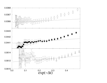
Table 4.2: The one-particle spectrum and the field normalization for lattices (A’) and (C’).

Figure 4.2: The asymptotic behavior of $\omega_{\rm eff}(\overline{p},t)$ as $t\to\infty$ on lattices (A’) (left) and (C’) (right). Empty circles refer to $\overline{p}=0$, filled squares to $\overline{p}=2\pi/L$ and triangles to $\overline{p}=6\pi/L$. The continuous lines are the best fitting curves of the form (3.3.18).

The one-particle spectrum $\omega(\overline{p})$ and the field normalization $Z(\overline{p})$ have been extracted from $C(\overline{p};t)$ on lattices (A’) and (C’) as explained in Sec. 3.3.2. For the relevant definitions see Eq. (3.3.13). The results of this computation are shown in Tab. 4.2. We verified that the effective quantities $\omega_{\rm eff}(\overline{p},t)$ and $Z_{\rm eff}(\overline{p},t)$ do not depend upon $t$ for $t\mathrel{\hbox to0.0pt{\lower 3.0pt\hbox{$\mathchar 536\relax$}\hss}\raise 2.0pt\hbox{$\mathchar 318\relax$}}\xi_{\rm exp}$. The values reported in Tab. 4.2 correspond to $t=8,\,24$ respectively on lattices (A’) and (C’).

In order to estimate the systematic error due to the fact that we use a finite value of $t$ we fitted $\omega_{\rm eff}(\overline{p},t)$ and $Z_{\rm eff}(\overline{p},t)$, taking into account the first correction to the $t\to\infty$ behavior. The procedure has been explained in the previous Chapter, see Sec. 3.3.2. The fitting form was of the type (3.3.18). The results of this fit are shown in Fig. 4.2. The corresponding estimates for the systematic errors on the values of $\omega(\overline{p}=0)$ quoted in Tab. 4.2 are about $0.3\div 0.4\cdot 10^{-4}$, on both lattices (A’) and (C’). In general we verified the systematic error to be of the same order as (or smaller than) the statistical one.

The exponential correlation length $\xi_{\rm exp}=m^{-1}$ obtained from the data of Tab. 4.2 is

$$\xi_{\rm exp}=6.831(2),\;27.325(24)\,,$$ (4.4.16)

respectively for lattices (A’) and (C’). Notice that $\xi_{\rm exp}({\rm C^{\prime}})\approx 2\xi_{\rm exp}({\rm B})$ and $\xi_{\rm exp}({\rm B})\approx 2\xi_{\rm exp}({\rm A^{\prime}})$ with deviations of (relative) order $10^{-3}$. Comparing the numerical results obtained on these three lattices, we can carefully verify the scaling of correlation functions.

4.4.3 Corrections to Scaling

Let us consider the normalized functions $\widehat{G}^{(l)}(t,x;\overline{p},\overline{q};\infty)$, where the on-shell limit $t_{s}\to\infty$ has been taken. We expect the quantity

$$\sqrt{4\omega(\overline{p})\omega(\overline{q})}Z_{L}^{-1}\widehat{G}^{(l)}(t,x;\overline{p},\overline{q};\infty)$$ (4.4.17)

to have a finite continuum limit, i.e. $g_{L}\to 0$ with $mx$, $mt$, $\overline{p}/m$ and $\overline{q}/m$ fixed. This limit is approached with $O(a^{2}\log^{p}a)$ corrections [103, 104, 105]. Renormalization group implies the following scaling form in the continuum limit:

$$\sqrt{4\omega(\overline{p})\omega(\overline{q})}\widehat{G}^{(l)}(t,x;\overline{p},\overline{q};\infty)=V(g_{L})\,{\cal G}^{(l)}(mt,mx;\overline{p}/m,\overline{q}/m)+O(m^{2},t^{-2},x^{-2},\overline{p}^{2},\overline{q}^{2})\,,$$

(4.4.18)

where

$$V(g_{L})=g_{L}^{-\gamma^{L}_{0}/\beta_{0}}\exp\left\{-\int_{0}^{g_{L}}\left[\frac{\gamma^{L}(z)}{\beta^{L}(z)}+\frac{\gamma^{L}_{0}}{\beta_{0}z}\right]\right\}\,.$$ (4.4.19)

Let us now fix $g_{L}$ and $g_{L}^{\prime}$ in such a way that $m(g_{L})/m(g_{L}^{\prime})=\theta$ is kept fixed. From Eq. (4.4.18), and using the fact that $\omega(\overline{p})\to\sqrt{m^{2}+\overline{p}^{2}}$ in the continuum limit, we get:

$$\frac{\widehat{G}^{(l)}(\theta t,\theta x;\overline{p},\overline{q};\infty|g_{L}^{\prime})}{\widehat{G}^{(l)}(t,x;\theta\overline{p},\theta\overline{q};\infty|g_{L})} = \theta\,U(g_{L},g^{\prime}_{L})+\mbox{corrections}\;,$$ (4.4.20)

$$U(g_{L},g^{\prime}_{L}) \equiv \exp\left\{-\int_{g_{L}}^{g_{L}^{\prime}}\!dz\left[\frac{\gamma^{L}(z)}{\beta^{L}(z)}\right]\right\}\,.$$ (4.4.21)

The r.h.s. of Eq. (4.4.20) is independent of $t$, $x$, $\overline{p}$, $\overline{q}$, and even of the particular ($l=0,1,2$) correlation function, up to $O(a^{2}\log^{p}a)$ lattice artifacts. Since we adopted lattice regularization, Eq. (4.4.20) is meaningful for some $t,x\in\mathbb{Z}$ only if $\theta$ is a rational number.

Figure 4.3: The scaling ratio (4.4.20) for $l=2$ and $\theta=2$, along the directions $x=0$ and $t=0$. We use lattices (A’) and (B) on the left, and lattices (B) and (C’) on the right. Empty circles ($\circ$) refer to $\overline{p}=0$, filled squares ($\blacksquare$) to $\overline{p}=2\pi/L$.

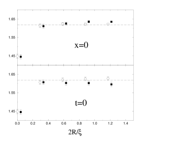
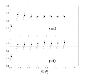
Let us now turn to the numerical results, which are shown in Fig. 4.3. We considered the ratio on the l.h.s. of Eq. (4.4.20) for $l=2$ and $\theta=2$. In the left column we use lattices (A’) and (B) (i.e. $1/g_{L}=1.39838694$ and $1/g_{L}^{\prime}=1.54$); in the right column lattices (B) and (C’) (i.e. $1/g_{L}=1.54$ and $1/g_{L}^{\prime}=1.66135987$). We used $\overline{p}=\overline{q}=2\pi n/L$, $n=0,1,2$. In Eq. (4.4.20) we have to extrapolate the normalized correlation function $\widehat{G}^{(l)}(\dots;2t_{s})$ for $t_{s}\to\infty$. We verified that the ratio on the left-hand side of Eq. (4.4.20) does not depend upon the chosen value of $t_{s}$ among the ones for which $\widehat{G}^{(2)}$ was computed, see Sec. 4.4.1. The data presented refer to $t_{s}=10,16,30$ respectively for lattices (A’), (B), (C’). In Fig. 4.3 we plot our numerical results for the ratio (4.4.20) along the directions $x=0$ and $t=0$.

The plots obtained with lattices (B) and (C’) (right column) show clear evidence of scaling at error bars level (about $1\div 2\%$ depending upon the chosen $t,x$ and $\overline{p}$) as soon as $(t,x)\neq(0,0)$. From Eq. (4.4.20), neglecting corrections to scaling we obtain the estimate $U(g_{L},g_{L}^{\prime})=0.83(2)$. Four-loop (three-loop, two-loop) lattice perturbation theory yields $U(g_{L},g_{L}^{\prime})=0.84251$ ($0.84807$, $0.85310$). Improved perturbation theory yields $U(g_{L},g_{L}^{\prime})=0.81666(6)$ ($0.81751(6)$, $0.81614(6)$).

Lattices (A’) (B) (Fig. 4.3 left column) show approximate scaling for $(t,x)\neq(0,0)$. The horizontal lines would imply $U(g_{L},g_{L}^{\prime})\sim 0.810(5)$ (we report the statistical error which is roughly independent of the particular $(t,s)$ point, rather than the systematic error due to scaling corrections). Four-loop (three-loop, two-loop) lattice perturbation theory yields $U(g_{L},g_{L}^{\prime})=0.79837$ ($0.80716$, $0.81570$). With improved perturbation theory we get $U(g_{L},g_{L}^{\prime})=0.77277(4)$ ($0.77420(4)$, $0.77217(4)$). Small scaling corrections could be suggested by the points around $t=4$ or $x=4$. This discrepancies are not completely significant from a statistical point of view (about $1\%$, while statistical errors are approximatively $0.5\%$).

Moreover, we remark that lattice perturbation theory gives unexpectedly good estimates for the constant $U(g_{L},g_{L}^{\prime})$ on lattices (B)-(C’). This is probably due to the fact that $U(g_{L},g_{L}^{\prime})$ is finite (indeed $U(g_{L},g_{L}^{\prime})\to 0$) in the continuum limit ($g_{L},g_{L}^{\prime}\to 0$ at $m(g_{L})/m(g_{L}^{\prime})=\theta$ fixed).

Notice that both using lattices (A’) and (B), and using lattices (B) and (C’), the relation $m(g_{L})/m(g_{L}^{\prime})=2$ is not exactly satisfied, the discrepancy being of order $10^{-3}$. In order to check whether our conclusion could be changed by a better tuning of the bare lattice couplings, we reweighted our numerical data on lattice (A’) at $g_{L}^{-1}=1.39791766$. At this coupling we get $\xi_{\rm exp}=6.816(2)$. The results for the scaling ratio (4.4.20) cannot be distinguished from the ones shown in Fig. 4.3.

In the following Subsections we shall use the OPE method for computing renormalization constants and renormalized matrix elements from lattice data. The results of the present Subsection give us a rough idea of the relevance of lattice artifacts in these computations. As soon as we avoid products of lattice fields at coincident points, we expect these errors to be about $1\%$ on lattice (A), and to be compatible with statistical uncertainties on lattices (B) and (C). We shall see that these effects are negligible with respect to other sources of error (in particular the systematic error due to the perturbative truncation of the Wilson coefficients). As explained at the beginning of this Section, we shall put a short distance cutoff $\rho$ on our fitting region (i.e. we take $\rho<r<R$). In order to avoid fields products at coincident points, we shall always consider $\rho>0$. Varying $\rho$ (in particular we considered $\rho=0.5$ and $\rho=1.5$, keeping $R>\rho+2$ fixed) does not change much the results of the fits. These small changes (always much smaller than estimated systematic errors) can be ascribed to asymptotic scaling corrections, rather than to scaling corrections. In particular, increasing $\rho$ produce an effect of the same sign as increasing $R$.

Motivated by this discussion, we shall present, in the following Subsections, the results obtained fixing $\rho=0.5$.

4.4.4 Field-Renormalization Constant

We can apply the OPE approach to the computation of the field-renormalization constant. The method can be easily extended to any other composite operator ${\cal A}$. In Sec. 4.4.6 we shall apply it to the symmetric traceless operator $S_{0}^{ab}$, see Eq. (4.2.5). The idea is to compute numerically a short distance product of the type

$$\langle 1|{\cal A}(x){\cal A}(-x)|2\rangle\sim W_{\cal O}(x)\langle 1|{\cal O}|2\rangle+\dots\,,$$ (4.4.22)

such that the matrix element on the right-hand side is known. Enforcing the validity of the OPE allows to compute the renormalization constant of $Z_{L,{\cal A}}$.

In this Subsection we want to compute the field-renormalization constant $Z_{L}$. We will apply the method described above with ${\cal A}=\sigma^{a}$. The simplest choice is to consider the two-point function. This is equivalent to choosing the states $\langle 1|$ and $|2\rangle$ in Eq. (4.4.22) to be the vacuum state. From Eq. (4.2.2) we obtain

$$\langle\mbox{\boldmath$\sigma$}_{RGI}(x)\cdot\mbox{\boldmath$\sigma$}_{RGI}(-x)\rangle={\cal F}^{(0)}_{RGI,0}(\overline{g}_{\zeta}(r);\zeta)+\widehat{\cal F}^{(0)}_{RGI,2}(\overline{g}_{\zeta}(r);\zeta)r^{2}\langle[(\partial\mbox{\boldmath$\sigma$})^{2}]_{RGI}\rangle+O(x^{4})\,,$$

(4.4.23)

where we used Eq. (2.3.16) to express the vacuum expectation value of the energy-momentum tensor in terms of $\langle(\partial\mbox{\boldmath$\sigma$})^{2}\rangle$, and Eq. (2.3.13) to eliminate the non-invariant operator $\alpha$. The RGI Wilson coefficients are obtained from Eqs. (4.2)–(4.2.9) using the formulae of Sec. 2.7:

$${\cal F}^{(0)}_{RGI,0}(\overline{g};1) = \overline{g}^{-(N-1)/(N-2)}\left\{1+\frac{N-1}{2\pi(N-2)}\overline{g}-\frac{(N-1)(N^{2}-6N+6)}{16\pi^{2}(N-2)^{2}}\overline{g}^{2}+\right.$$ (4.4.24)

$$+\frac{(N-1)}{192\pi^{3}(N-2)^{3}}[N^{4}(8\zeta(3)-7)+N^{3}(-54\zeta(3)+56)+$$

$$\quad\quad+6N^{2}(20\zeta(3)-29)+N(-88\zeta(3)+256)-148]\overline{g}^{3}\Bigg{\}}\,,$$

$$\widehat{\cal F}^{(0)}_{RGI,2}(\overline{g};1) = -\overline{g}^{-(N-1)/(N-2)}\left\{1+\frac{N^{2}-4N+5}{2\pi(N-2)}\overline{g}\right\}\,.$$ (4.4.25)

Figure 4.4: Monte Carlo data for the isovector correlation function, and OPE predictions. Different symbols refer to different lattices: empty triangles ($\triangle$) to lattice (A), filled circles ($\bullet$) to lattice (B) and stars ($\ast$) to lattice (C). The continuous (dotted) line is the best fitting curve including (not including) power corrections.

Figure 4.5: The results of the fit of the two-point function. In the left column (frames (A), (B) and (C)) we show ${\cal Z}(\rho,R)$, in the right column (frames (A’), (B’) and (C’)) ${\cal W}(\rho,R)$. Graphs (A) and (A’) refer to lattice (A), (B) and (B’) to lattice (B), (C) and (C’) to lattice (C). Different symbols correspond to different fitting form: stars ($\ast$) to Eq. (4.4.32) with power corrections; diamonds ($\Diamond$) to Eq. (4.4.32) without power corrections; dashed lines to Eq. (4.4.32) without power corrections and two-loop Wilson coefficient; continuous lines to Eq. (4.4.32) without power corrections and one-loop Wilson coefficient. In the first two cases we plot the value obtained at $\zeta e^{\gamma}=1$ and the systematic error bars, obtained by varying $\zeta$. In the other cases we show the maximum and the minimum values obtained in the chosen range of $\zeta$. Statistical errors are negligible in these plots and we do not report them.

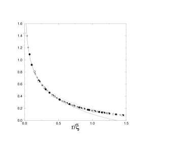
The lattice fields renormalize as follows, see Sec. 2.5,

$$\mbox{\boldmath$\sigma$}(x)=Z_{L}^{-1/2}(g,g_{L})\mbox{\boldmath$\sigma$}_{x}\,,$$ (4.4.26)

where we emphasized the dependence of $Z_{L}$ upon $g_{L}$ and $g$, i.e., in more physical terms, upon $\Lambda a$ and $\Lambda/\mu$. This dependence can be predicted using RG. In fact the following equations hold:

$$\left[\beta(g)\frac{\partial}{\partial g}+\gamma(g)\right]Z_{L} = 0\,,$$ (4.4.27)

$$\left[\beta_{L}(g)\frac{\partial}{\partial g_{L}}-\gamma_{L}(g_{L})\right]Z_{L} = 0\,.$$ (4.4.28)

These are simply the definitions of the continuum and lattice anomalous dimensions $\gamma(g)$ and $\gamma_{L}(g_{L})$. The general solution of the above equations reads

$$Z_{L}(g,g_{L})=\widehat{Z}\cdot g^{-\gamma_{0}/\beta_{0}}\exp\left[\int_{0}^{g}\!dx\left(\frac{\gamma(x)}{\beta(x)}+\frac{\gamma_{0}}{\beta_{0}x}\right)\right]\cdot g_{L}^{\gamma_{0}/\beta_{0}}\exp\left[-\int_{0}^{g_{L}}\!dx\left(\frac{\gamma_{L}(x)}{\beta_{L}(x)}+\frac{\gamma_{0}}{\beta_{0}x}\right)\right]\,.$$

(4.4.29)

The constant $\widehat{Z}$ is easily fixed. Noticing that $Z_{L}(g,g_{L})=1+O(g)$ and $g_{L}=g+O(g^{2})$, we obtain

$$\widehat{Z}=1\,.$$ (4.4.30)

As in the rest of this Chapter we have different attitudes towards different terms in Eq. (4.4.29). The lattice factor $g_{L}^{\gamma_{0}/\beta_{0}}\dots$ can be computed in perturbation theory. However, since lattice perturbation theory is not well behaved, we are interested in computing it non-perturbatively. The continuum factor $g^{-\gamma_{0}/\beta_{0}}\dots$ can be computed in perturbation theory too. In this case, we assume that we are interested in an energy scale $\mu$ which is high enough for making the perturbative calculation reliable (recall that $g(\mu)\to 0$ as $\mu\to\infty$).

Notice that adsorbing the continuum factor $g^{\gamma_{0}/\beta_{0}}\dots$ in the definition of $\sigma$ yields the (finite) RGI field operator $\mbox{\boldmath$\sigma$}_{RGI}(x)$. Motivated by the above discussion, we shall compute the renormalization constant $Z_{L,RGI}(g_{L})$, defined by: $\mbox{\boldmath$\sigma$}_{RGI}(x)=Z_{L,RGI}^{-1/2}(g_{L})\mbox{\boldmath$\sigma$}_{x}$. Its explicit RG expression is easily obtained from Eq. (4.4.29):

$$Z_{L,RGI}(g_{L})=g_{L}^{\gamma_{0}/\beta_{0}}\exp\left[-\int_{0}^{g_{L}}\!dx\left(\frac{\gamma_{L}(x)}{\beta_{L}(x)}+\frac{\gamma_{0}}{\beta_{0}x}\right)\right]\,.$$ (4.4.31)

Being written in terms of RGI fields, Eq. (4.4.23) gives access to $Z_{L,RGI}(g_{L})$. We use the following fitting form for the two point function:

$$G(t,x)={\cal F}^{(0)}_{RGI,0}(\overline{g}_{\zeta}(r/2);\zeta){\cal Z}+\widehat{\cal F}^{(0)}_{RGI,2}(\overline{g}_{\zeta}(r/2);\zeta)(mr/2)^{2}{\cal W}\,.$$ (4.4.32)

As always we restrict the fit to the region $\rho\leq r\leq R$. The parameter ${\cal Z}$ gives an estimate of $Z_{L,RGI}(g_{L})$. The parameter ${\cal W}$ could be called a “spin-wave” condensate. However we do not expect to be able to determine the value of $\langle[(\partial\mbox{\boldmath$\sigma$})^{2}]_{RGI}\rangle$ from it. In fact $(\partial\mbox{\boldmath$\sigma$})^{2}$ mixes with the identity operator and the remarks of Sec. 4.1.2 apply to this case. We should determine the Wilson coefficient ${\cal F}^{(0)}_{RGI,0}(\overline{g}_{\zeta}(r/2);\zeta)$ up to terms of order $m^{2}r^{2}$ for Eq. (4.4.23) to define $\langle[(\partial\mbox{\boldmath$\sigma$})^{2}]_{RGI}\rangle$ unambiguously.

For each case we repeated the fit with and without the power-correction term ${\cal W}$. This gives a feeling of how good is the truncation of the OPE in Eq. (4.4.23).

In Fig. 4.4 we present a scaling plot of Monte Carlo data for $G(t,x)$ together with the best fitting curves with and without power corrections. For sake of clarity we plotted only the values of $G(t,x)$ obtained along the time direction $(t,x)=(t,0)$, and along the diagonal $(t,x)=(t,t)$. We rescaled the data using the estimated values of $Z_{L,RGI}(g_{L})$, i.e. $\widehat{\cal Z}^{*}$, see Tab. 4.3 and discussion below. The data collapse on a single curve showing a clear evidence of scaling. The dotted curve (no power corrections) simply reports ${\cal F}^{(0)}_{RGI,0}(\overline{g}_{\zeta}(r/2);\zeta)$. In the continuous curve we add the power correction $\widehat{\cal F}^{(0)}_{RGI,2}(\overline{g}_{\zeta}(r/2);\zeta)(mr/2)^{2}\widehat{\cal W}^{*}/\widehat{\cal Z}^{*}$, with $\widehat{\cal W}^{*}$ and $\widehat{\cal Z}^{*}$ obtained on lattice (C).

In Fig. 4.5 we show the best fitting parameters ${\cal Z}(\rho,R)$ and ${\cal W}(\rho,R)$ on lattices (A), (B) and (C). In all the cases we kept $\rho=0.5$ fixed (this excludes only the point $(t,x)=(0,0)$ from the fit), and we varied $R$. Statistical errors are negligible in these plots and we do not report them.

The estimates ${\cal W}(\rho,R)$ are reported in frames (A’), (B’), (C’). These graphs do not allow any reliable evaluation of the expectation value $\langle[(\partial\mbox{\boldmath$\sigma$})^{2}]_{RGI}\rangle$. For $R\mathrel{\hbox to0.0pt{\lower 3.0pt\hbox{$\mathchar 536\relax$}\hss}\raise 2.0pt\hbox{$\mathchar 318\relax$}}0.7\,\xi_{\rm exp}$ systematic errors are of the same order as the estimate itself. For $R\mathrel{\hbox to0.0pt{\lower 3.0pt\hbox{$\mathchar 536\relax$}\hss}\raise 2.0pt\hbox{$\mathchar 316\relax$}}0.7\,\xi_{\rm exp}$ systematic errors begin to shrink but ${\cal W}(\rho,R)$ shows a strong $R$ dependence. Indeed ${\cal W}(\rho,R)$ seems to diverge as $R\to 0$. This can be easily understood if we assume that we are effectively fitting higher loops (which go as $r^{0}$ as $r\to 0$) with a term of the type ${\cal W}r^{2}$.

$\widehat{\cal Z}^{*}$ $\widehat{Z}_{4\,loop}\,\{\widehat{Z}_{3\,loop},\,\widehat{Z}_{2\,loop}\}$ $\widehat{Z}^{bpt}_{4\,loop}\,\{\widehat{Z}^{bpt}_{3\,loop},\,\widehat{Z}^{bpt}_{2\,loop}\}$ lattice (A) $0.67[1]$ $0.957\,\{0.916,\,0.861\}$ $1.075\,\{1.068,\,1.082\}$ lattice (B) $0.559[5]$ $0.918\,\{0.889,\,0.843\}$ $0.9990\,\{0.9944,\,1.0048\}$ lattice (C) $0.468[3]$ $0.924\,\{0.900,\,0.861\}$ $\,0.976\{0.973,\,0.981\}$

Table 4.3: The OPE result $\widehat{\cal Z}^{*}$ for the field-renormalization constant $Z_{L,RGI}(g_{L})$ and the corresponding perturbative estimates for the constant $\widehat{Z}$ defined in Eq. (4.4.33). We used lattice perturbation theory in the third column and improved (boosted) perturbation theory in the fourth column. These values should be compared with the exact result $\widehat{Z}=1$.

In graphs (A), (B), (C) we report the results for ${\cal Z}(\rho,R)$. The estimates obtained including the power-correction term in Eq. (4.4.32) show a quite mild $R$ dependence and very small systematic errors which are roughly $R$-independent. These values of ${\cal Z}(\rho,R)$ are not constant within systematic error bars. The reason is probably that the fitting parameter ${\cal W}$ mimics the effects of higher loops in ${\cal F}^{(0)}_{RGI,0}(\overline{g}_{\zeta}(r/2);\zeta)$ and reduces the scheme dependence of the result. The estimates obtained without power corrections show larger systematic errors and are flat within the systematic error bars. Systematic errors decrease as $R\to 0$.

In the same graphs we reported the analogous estimates (obtained without power corrections) with ${\cal F}^{(0)}_{RGI,0}(\overline{g}_{\zeta}(r/2);\zeta)$ computed in one-loop and two-loop perturbation theory. Our method to assess systematic errors seems to be consistent. Finally the difference between the results for ${\cal Z}(\rho,R)$ obtained with or without power corrections are quite small.

$R$ $R/\xi_{\rm exp}$ ${\cal Z}(\rho,R)[\mbox{syst. }\kappa=1.5]\,[\kappa=2]\,[\kappa=2.5]$ 3-loop 2-loop 1-loop $3.5$ $0.13$ $0.4726[14]\,[25]\,[33]$ $0.469[4]\,[8]\,[12]$ $0.46[2]\,[4]\,[5]$ $5.5$ $0.20$ $0.468[2]\,[3]\,[5]$ $0.464[5]\,[11]\,[16]$ $0.46[2]\,[4]\,[7]$ $7.5$ $0.28$ $0.464[3]\,[4]\,[7]$ $0.459[7]\,[13]\,[20]$ $0.45[3]\,[5]\,[8]$ $9.5$ $0.35$ $0.459[3]\,[6]\,[9]$ $0.453[8]\,[17]\,[26]$ $0.45[3]\,[6]\,[9]$ $15.5$ $0.57$ $0.447[6]\,[13]\,[21]$ $0.439[13]\,[28]\,[46]$ $0.43[4]\,[8]\,[13]$

Table 4.4: We compare different estimates of the systematic error on the field renormalization constant. Here we consider the data obtained on lattice (C) and use the fitting form (4.4.32) without power corrections.

We summarize our results for $Z_{L,RGI}(g_{L})$ in Tab. 4.3. The values of $\widehat{\cal Z}^{*}$ correspond to ${\cal Z}(\rho,R)$ at $R=2.5$, $3.5$, $5.5$ on lattices (A), (B) and (C). In the third column we compute the constant $\widehat{Z}$, see Eq. (4.4.29), using the relation

$$\widehat{Z}=Z_{L,RGI}(g_{L})\cdot g_{L}^{-\gamma_{0}/\beta_{0}}\exp\left[\int_{0}^{g_{L}}\!dx\left(\frac{\gamma_{L}(x)}{\beta_{L}(x)}+\frac{\gamma_{0}}{\beta_{0}x}\right)\right]\,$$ (4.4.33)

and four-loop (three-loop, two-loop) perturbation theory. In the last column we repeat the same calculation using improved perturbation theory. The results for $\widehat{Z}$ seem to scale well (i.e. they are approximatively $g_{L}$-independent) for the lattices (B) and (C). A little discrepancy remains for lattice (A). Nevertheless, even at four loops, the outcome of bare perturbation theory is about $7-8\%$ away from the correct value $\widehat{Z}=1$. Improved perturbation theory yields a better agreement. For the largest lattice the discrepancy is about the $2\%$, which is not too far from the estimated systematic error (approximatively the $1\%$).

Let us now try to judge our determination of systematic errors and in particular our choice of $\kappa$. We shall concentrate on lattice (C), since it allows to investigate a larger range of distances. In Tab. 4.4 we report the results for ${\cal Z}(\rho,R)$ and the corresponding systematic error for several values of $R$ and $\kappa$. The fitting form (4.4.32) without power correction was adopted. The Wilson coefficient was computed in three-loop, two-loop, and one-loop perturbation theory. If we look at a fixed value of $R$ in this table it seems that perturbation theory converges very well and that, fixing $\kappa=2$, we are overestimating the systematic errors: $\kappa=1.5$ could appear a more realistic choice. However if we vary $R$ and consider the systematic error obtained with $\kappa=1.5$ we realize that ${\cal Z}(\rho,R)$ is by no means flat. We deduce that $\kappa=2$ is not too cautious and gives a good (very rough) idea of the systematic errors.

4.4.5 Symmetric Operator

As we explained in Sec. 4.4.1, we are interested in computing the matrix elements of the bare lattice operator $\sigma^{a}\sigma^{b}-\delta^{ab}/N$ between one-particle states. In order to accomplish this task, we considered the three-point function $C^{(2)}(\overline{p},\overline{q};2t)$ defined in Eq. (4.4.11). The matrix element can be extracted from the corresponding normalized function $\widehat{C}^{(2)}(\overline{p},\overline{q};2t)$ as follows:

$$\langle\overline{p},c|\sigma^{a}\sigma^{b}-\frac{\delta^{ab}}{N}|\overline{q},d\rangle=T_{N}^{ab,cd}\sqrt{4\omega(\overline{p})\omega(\overline{q})}\lim_{t\to\infty}\widehat{C}^{(2)}(\overline{p},\overline{q};2t)\,,$$ (4.4.34)

where

$$T_{N}^{ab,cd}=\frac{N}{(N-1)(N+2)}\left(\delta^{ac}\delta^{bd}+\delta^{ad}\delta^{bc}-2\delta^{ab}\delta^{cd}/N\right)\,.$$ (4.4.35)

The numerical results for $\widehat{C}^{(2)}(\overline{p},\overline{p};2t)$ are constant (within statistical errors) for $t\mathrel{\hbox to0.0pt{\lower 3.0pt\hbox{$\mathchar 536\relax$}\hss}\raise 2.0pt\hbox{$\mathchar 318\relax$}}\xi_{\rm exp}$.

$\overline{p}$	lattice (A)	lattice (B)	lattice (C)
$0$	$0.7888(13)$	$0.5862(20)$	$0.4309(29)$
$2\pi/L$	$0.7877(20)$	$0.5855(26)$	$0.4311(36)$
$4\pi/L$	$0.7915(95)$	$0.573(12)$	$0.421(17)$
$6\pi/L$	$0.757(13)$	$0.581(19)$	$0.462(23)$

Table 4.5: The numerical estimates of $2\sqrt{\overline{p}^{2}+m^{2}}\,\widehat{C}^{(2)}(\overline{p},\overline{p};2t)$. For $\overline{p}=0,\dots,4\pi/L$, $t=9,18,36$ respectively on lattice (A), (B) and (C). For $\overline{p}=6\pi/L$, $t=7,14,28$ on the same lattices.

In Tab. we report the numerical estimates for $2\sqrt{\overline{p}^{2}+m^{2}}\,\widehat{C}^{(2)}(\overline{p},\overline{p};2t)$ obtained on lattices (A), (B) and (C), respectively for $t=9$ ($t=7$ for $\overline{p}=6\pi/L$), $18$ ($t=14$ for $\overline{p}=6\pi/L$) and $36$ ($t=28$ for $\overline{p}=6\pi/L$).

Figure 4.6: The asymptotic behaviour of $2\sqrt{\overline{p}^{2}+m^{2}}\,\widehat{C}^{(2)}(\overline{p},\overline{p};2t)$ on lattices (A) (left) and (C) (right). Empty circles refer to $\overline{p}=0$, and filled squares to $\overline{p}=2\pi/L$. Continuous and dashed lines are the best fitting curves of the form (4.4.37) for (respectively) $\overline{p}=0$ and $\overline{p}=2\pi/L$. For sake of clarity we show the data obtained on lattice (C) only for $t\leq 36$.

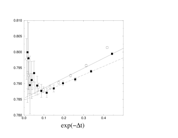
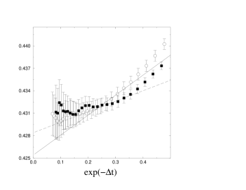
In order to verify the “contamination” due to higher states, we adopt the same method we used in the computation of the one-particle spectrum, see Sec. 3.3.2. The expected behaviour of $\widehat{C}^{(2)}(\overline{p},\overline{q};2t)$ in the large $t$ limit is

$$\widehat{C}^{(2)}(\overline{p},\overline{q};2t)=\widehat{C}^{(2)}(\overline{p},\overline{q};\infty)+D(\overline{p},\overline{q};t)e^{-\Delta(\overline{p})t}+D(\overline{q},\overline{p};t)e^{-\Delta(\overline{q})t}+\dots\,,$$ (4.4.36)

where we made the same approximations as for the spectrum, namely we neglected terms of order $e^{-\omega(\overline{p})T}$, and multi-particle states involving more than three particles. The gap $\Delta(\overline{p})$ is given by Eq. (3.3.17). In the thermodynamic ($L\to\infty$) limit, the coefficients $D(\overline{q},\overline{p};t)$ are slowly varying (power-like) functions of $t$. Analogously to what we did in Sec. 3.3.2, we shall neglect the $t$-dependence of the coefficients $D(\overline{q},\overline{p};t)$. We fitted our data using the form

$$2\sqrt{\overline{p}^{2}+m^{2}}\,\widehat{C}^{(2)}(\overline{p},\overline{p};2t)=\widehat{C}^{(2)}_{*}(\overline{p},\overline{q};\infty)+2D_{*}(\overline{p},\overline{p};t)e^{-\Delta(\overline{p})t}\,.$$ (4.4.37)

In Fig. 4.6 we plot $2\sqrt{\overline{p}^{2}+m^{2}}\,\widehat{C}^{(2)}(\overline{p},\overline{p};2t)$ versus $e^{-\Delta(\overline{p})t}$ on lattices (A) and (C) for $\overline{p}=2\pi n/L$, $n=0,\,1$. The estimated systematic error on the results of Tab. 4.5 is about $2\cdot 10^{-3}$,$2\cdot 10^{-3}$,$3\cdot 10^{-3}$,$6\cdot 10^{-2}$, respectively for $\overline{p}=0,\dots,6\pi/L$.

Notice that, for kinematical reasons, in the continuum limit $\langle\overline{p},c|\sigma^{a}\sigma^{b}-\delta^{ab}/N|\overline{p},d\rangle$ does not depend upon $\overline{p}$. The results of Tab. 4.5 verify this prediction within the statistical errors. The only statistically significant discrepancy occurs at $\overline{p}=6\pi/L$ on lattice (A). It is plausible to explain this discrepancy as a scaling correction.

4.4.6 Renormalization of the Symmetric Operator

Let us now come to the problem of renormalizing the lattice results obtained in the previous Section. This is a necessary step in order to check the results of Sec. 4.4.9, where we shall adopt the OPE method to compute the matrix elements of the renormalized operator $\left[S_{0}\right]_{\overline{MS}}$, see Eq. (4.2.5).

We have seen in Sec. 4.4.4 that improved (boosted) perturbation theory yields the field-renormalization constant with $1-2\%$ of systematic error on lattice (C). Now we have to compute the renormalization constant for the symmetric operator $S_{0}$. We shall use perturbation theory at first. Next, we shall switch to the OPE non-perturbative method, see Sec. 4.4.4, in order to have more reliable results. We shall see that, in this case, lattice perturbation theory (even if improved) does not give an approximation as good as it does for the field-renormalization constant.

We proceed as in Sec. 4.4.4. Let us consider an operator ${\cal O}$ renormalizing multiplicatively: $\left[{\cal O}\right]_{\overline{MS}}=Z_{L}^{\cal O}{\cal O}_{L}$. The corresponding RGI operator ${\cal O}_{RGI}$ is easily given in terms of its lattice counterpart: ${\cal O}_{RGI}=Z_{L,RGI}^{\cal O}{\cal O}_{L}$. RG considerations yield:

$$Z_{L,RGI}^{\cal O}=g_{L}^{\gamma_{0}/\beta_{0}}\exp\left[-\int_{0}^{g_{L}}\!dx\left(\frac{\gamma^{\cal O}_{L}(x)}{\beta_{L}(x)}+\frac{\gamma^{\cal O}_{0}}{\beta_{0}x}\right)\right]\,,$$ (4.4.38)

where $\gamma^{\cal O}_{L}(g)$ are the lattice anomalous dimensions of the operator ${\cal O}$, see Sec. 2.6.

	${\cal S}_{3\,loop}\,\{{\cal S}_{2\,loop}\}$	${\cal S}^{bpt}_{3\,loop}\,\{{\cal S}^{bpt}_{2\,loop}\}$
lattice (A)	$1.640(3)\,\{1.800(3)\}$	$1.302(2)\,\{1.277(2)\}$
lattice (B)	$1.674(6)\,\{1.809(6)\}$	$1.414(5)\,\{1.393(5)\}$
lattice (C)	$1.576(11)\,\{1.685(11)\}$	$1.402(9)\,\{1.384(9)\}$

Table 4.6: The perturbatively-renormalized matrix element of the RGI symmetric operator, see Eq. (4.4.39). While in the second column we use bare lattice perturbation theory, in the third we use the improved expansion parameter $g_{E}$.

In Tab. 4.6 we report the results for

$${\cal S}\equiv\frac{1}{N}\sum_{a,b}\langle\overline{p},a|\left[S^{ab}_{0}\right]_{RGI}|\overline{p},b\rangle\,,$$ (4.4.39)

obtained from the data of Tab. 4.5 using Eqs. (4.4.34) and (4.4.38). The lattice anomalous dimensions are known in three-loop perturbation theory [106]. The bare matrix element has been obtained from the $\overline{p}=0$ data at of Tab. 4.5.

Figure 4.7: Monte Carlo data for the isotensor correlation function, and OPE predictions. Empty triangles ($\triangle$) refer to lattice (A), filled circles ($\bullet$) to lattice (B), and stars ($\ast$) to lattice (C). The Monte Carlo data are rescaled using the non-perturbative renormalization constant, see Tab. 4.7, right column. The continuous line corresponds to the leading term of the OPE.

Figure 4.8: The $R$ dependence of the fitting parameter $\widehat{\cal Z}^{(2)}(\rho,R)$, see Eq. (4.4.43). The three graphs (A), (B) and (C) have been obtained, respectively, on lattices (A), (B) and (C). We used three-loop (diamonds, $\Diamond$), and two-loop (dashed lines) perturbation theory in the computation of the Wilson coefficient. In the first case we plot the value obtained at $\zeta e^{\gamma}=1$ and the systematic error bars. In the second one we show the maximum and the minimum values obtained in the chosen range of $\zeta$.

The renormalized matrix elements of Tab. 4.6 seem to scale quite well. The results obtained with improved perturbation theory change by $1\%$ when passing from lattice (B) to lattice (C). They converge well when the order of the perturbative calculation is increased from two to three loops.

However, we would like to have a nonperturbative control over the renormalization constant of $S_{0}$. We shall consider the two-point function of this operator and proceed as in Sec. 4.4.4. We shall limit ourselves to the first term of the OPE:

$$\sum_{ab}\left\langle\left[S^{ab}_{0}\right]_{RGI}\!(x)\left[S^{ab}_{0}\right]_{RGI}\!(-x)\right\rangle=\frac{N-1}{N}{\cal E}_{RGI}(\overline{g}_{\zeta}(r);\zeta)+O(r^{2})\,.$$ (4.4.40)

Using the perturbative result of Eq. (4.2), and the general formulae of Sec. 2.7, we get

$${\cal E}_{RGI}(\overline{g};1) = \overline{g}^{-2N/(N-2)}\left\{1+\frac{N}{\pi(N-2)}\overline{g}-\frac{N(N^{2}-8N+4)}{8\pi^{2}(N-2)^{2}}\overline{g}^{2}+\right.$$

$$+\frac{N}{96\pi^{3}(N-2)^{3}}[N^{4}(10\zeta(3)-7)+N^{3}(-64\zeta(3)+50)+$$

$$\hskip 21.33955pt+12N^{2}(11\zeta(3)-12)+N(-80\zeta(3)+264)-16(\zeta(3)+11)]\overline{g}^{3}\Bigg{\}}\,.$$

Let us recall our notation for the renormalization constants, focusing on the case at hand:

$$\left[\sigma^{a}\sigma^{b}-\frac{1}{Z}\frac{\delta^{ab}}{N}\right]_{RGI}=Z_{L,RGI}^{(0,2)}(g_{L})\left(\sigma^{a}_{x}\sigma^{b}_{x}-\frac{\delta^{ab}}{N}\right)\,.$$ (4.4.42)

Equations (4.4.40) and (4.4.42) motivate the following fitting form for the isotensor correlation function, see Eq. (4.4.12):

$$G_{T}(t,x)=\frac{N-1}{N}{\cal E}_{RGI}(\overline{g}_{\zeta}(r/2);\zeta){\cal Z}^{(2)}\,.$$ (4.4.43)

The fitting parameter ${\cal Z}^{(2)}$ gives an estimate of $Z_{L,RGI}^{(0,2)}(g_{L})^{-2}$. As in the other cases we use a fitting window $\rho\leq r\leq R$ to extract the best fitting parameter $\widehat{\cal Z}^{(2)}(\rho,R)$.

	$\widehat{\cal Z}^{(2),*}$	${\cal S}^{np}$
lattice (A)	$0.382[36]$	$1.277(2)[61]$
lattice (B)	$0.203[13]$	$1.300(4)[40]$
lattice (C)	$0.114[6]$	$1.275(8)[32]$

Table 4.7: The OPE estimates $\widehat{\cal Z}^{(2),*}$ for the constant $Z_{RGI,L}^{(0,2)}(g_{L})^{-2}$, and the corresponding non-perturbatively renormalized matrix element of the symmetric operator.

In Fig. 4.7 we show our Monte Carlo data for $G_{T}(t,x)$ in a scaling plot. The numerical results for $G_{T}(t,x)$ have been rescaled using the estimated renormalization constant $\widehat{\cal Z}^{(2),*}$, see Tab. 4.7 and discussion below. For sake of clarity we limit ourselves to showing the results obtained along the directions $(t,x)=(t,0)$ and $(t,x)=(t,t)$. Scaling is well verified on the three lattices. The continuous line corresponds to the leading OPE prediction $(N-1)/N\,{\cal E}_{RGI}(\overline{g}_{\zeta}(r/2);\zeta)$, with $\zeta e^{\gamma}=1$.

In Fig. 4.8 we show the $R$ dependence of the best fitting parameter $\widehat{\cal Z}^{(2)}(\rho,R)$ on lattices (A), (B) and (C). As in Sec. 4.4.4, we kept $\rho=0.5$ constant. In all the cases examined, the estimates $\widehat{\cal Z}^{(2)}(\rho,R)$ are flat within the systematic error bars as soon as $R\mathrel{\hbox to0.0pt{\lower 3.0pt\hbox{$\mathchar 536\relax$}\hss}\raise 2.0pt\hbox{$\mathchar 316\relax$}}\xi$. Notice that the estimated systematic errors on $\widehat{\cal Z}^{(2)}(\rho,R)$ are larger than in Sec. 4.4.4. This is not unexpected. In fact, in the present case, the Wilson coefficient is more strongly varying: as $\overline{g}\to 0$, ${\cal E}_{RGI}(\overline{g};\zeta)\sim\overline{g}^{-6}$, while ${\cal F}^{(0)}_{RGI,0}(\overline{g};\zeta)\sim\overline{g}^{-2}$ (these formulae hold for $N=3$). As a consequence, the parameter $\widehat{\cal Z}^{(2)}(\rho,R)$ is more strongly dependent upon the perturbative truncation than its counterpart $\widehat{\cal Z}(\rho,R)$.

In Tab. 4.7 we present our results for $Z_{L,RGI}^{(0,2)}(g_{L})^{-2}$, and the corresponding renormalized matrix elements for the symmetric operator, see Eq. (4.4.39). The values of $\widehat{\cal Z}^{(2),*}$ correspond to $\widehat{\cal Z}^{(2)}(\rho,R)$ at $R=1.5$, $2.5$, and $5.5$, respectively on lattices (A), (B) and (C). The renormalized matrix elements ${\cal S}^{np}$ are obtained computing the renormalization constant from $\widehat{\cal Z}^{(2),*}$, and using the bare lattice matrix elements of Tab. 4.5, $\overline{p}=0$. These results scale, i.e. they are $g_{L}$ independent, within systematic errors. Systematic errors get reduced as the lattice becomes finer. They are about the $3\%$ on lattice (C).

The results of Tab. 4.7 should be compared with the ones of Tab. 4.6 (we refer here to improved perturbation theory, i.e. to the rightmost column). In both cases we present the matrix element ${\cal S}$, defined in Eq. (4.4.39), and we use the bare lattice data of Tab. 4.5, obtained at $\overline{p}=0$. The only difference consists in the estimate of the renormalization constant. In both cases, looking at the two larger lattices, (B) and (C), the values of ${\cal S}$ show scaling (i.e. they are independent of $g_{L}$) at percent level. There is, however, a discrepancy between the determinations of Tab. 4.6 and of Tab. 4.7. This discrepancy is about the $10\%$ on lattice (C), and is not compatible with the systematic error of the OPE method.

A $10\%$ disagreement between improved perturbation theory and non-perturbative results is not unfrequent at these correlation lengths, see for instance Refs. [62, 87, 65]. Moreover the results of Tab. 4.7 agree with the ones obtained by applying the OPE method to the computation of the matrix element, see Sec. 4.4.9 and Tab. 4.10. This provides a strong check of the whole approach.

4.4.7 OPE in the Scalar Sector

In this Subsection we study the short-distance product of two elementary fields in the $O(N)$-scalar sector.

As a preliminary step, we rewrite the general form of the OPE, see Eq. (4.2.2), with two changes: we use RGI operators instead of $\overline{\rm MS}$ ones; we use operators with definite spin. Moreover,we focus on the $h\to 0$ limit of on-shell matrix elements. Using Eq. (2.3.16) for the trace of the energy-momentum tensor, we get (neglecting terms of order $r^{4}$):

$$\mbox{\boldmath$\sigma$}_{RGI}(x)\cdot\mbox{\boldmath$\sigma$}_{RGI}(-x) = {\cal F}^{(0)}_{RGI,0}(\overline{g}_{\zeta}(r);\zeta)\mbox{\boldmath{1}}+$$

$$\widehat{\cal F}^{(0)}_{RGI,1}(\overline{g}_{\zeta}(r);\zeta)x_{\mu}x_{\nu}\widehat{T}_{\mu\nu}+\widehat{\cal F}^{(0)}_{RGI,2}(\overline{g}_{\zeta}(r);\zeta)r^{2}\left[(\partial\mbox{\boldmath$\sigma$})^{2}\right]_{RGI}\,,$$

where $\widehat{T}_{\mu\nu}$ is the traceless energy-momentum tensor:

$$\widehat{T}_{\mu\nu}=T_{\mu\nu}-\frac{1}{2}\delta_{\mu\nu}\delta^{\alpha\beta}T_{\alpha\beta}\,.$$ (4.4.45)

The expressions for ${\cal F}^{(0)}_{RGI,0}$ and $\widehat{\cal F}^{(0)}_{RGI,2}$ have been already given in Sec. 4.4.4, see Eqs. (4.4.24) and (4.4.25). The last Wilson coefficient is easily obtained from Eq. (4.2.7):

$$\widehat{\cal F}^{(0)}_{RGI,1}(\overline{g};1)=-2\overline{g}^{-1/(N-2)}\left[1+\frac{N-1}{2\pi(N-2)}\overline{g}\right]\,.$$ (4.4.46)

We shall consider one-particle matrix elements of Eq. (4.4.7). Space-time symmetries impose several constraints on the matrix elements of the operators on the right-hand side. This yields a further check of our calculation. We adopt the following parametrization:

$$\langle\overline{p},a|\widehat{T}_{\mu\nu}|\overline{p},b\rangle = (2p_{\mu}p_{\nu}-p^{2}\delta_{\mu\nu})\delta^{ab}{\cal T}_{R}\,,$$ (4.4.47)

$$\langle\overline{p},a|[(\partial\mbox{\boldmath$\sigma$})^{2}]_{RGI}|\overline{p},b\rangle = -p^{2}{\cal E}_{R}\,,$$ (4.4.48)

where $p_{\mu}\equiv(i\sqrt{\overline{p}^{2}+m^{2}},\overline{p})$ and $p^{2}=p_{0}^{2}+p_{1}^{2}=-m^{2}$. Because of kinematical considerations both ${\cal T}_{R}$ and ${\cal E}_{R}$ do not depend upon $\overline{p}$. Moreover,invariance under space and time inversions implies that ${\cal T}_{R}$ and ${\cal E}_{R}$ are both real. Finally, e know the exact value of the expectation value of the energy-momentum tensor. Recalling the normalization (3.3.11) for one-particle states, we get ${\cal T}_{R}=1$.

Let us make a few elementary remarks concerning the status of the different terms appearing in Eq. (4.4.7). The operator $(\partial\mbox{\boldmath$\sigma$})^{2}$ has spin 0 and dimension 2. In the context of deep-inelastic scattering it would be called a “higher twist” . It mixes under renormalization with the identity operator. The Lorentz structure of the corresponding Wilson coefficients is the same: they are rotationally invariant. The remarks of Sec. 4.1.2 apply to this case. The matrix elements of $(\partial\mbox{\boldmath$\sigma$})^{2}$ cannot be determined from the expansion (4.4.7) unless we fix the coefficient ${\cal F}^{(0)}_{RGI,0}$ up to $O(r^{2})$. As a consequence, we do not expect to be able to compute the matrix elements of $(\partial\mbox{\boldmath$\sigma$})^{2}$, i.e. the parameter ${\cal E}$, see Eq. (4.4.48), with our method.

The traceless energy-momentum tensor $\widehat{T}_{\mu\nu}$ is instead a leading twist (spin 2, dimension 2) and can be determined from the expansion (4.4.7), although it is only a power correction. We could, for instance, consider the quantity:

$$S_{\mu\nu}(u)=\int\!\frac{d^{2}x}{2\pi x^{2}}\,\delta(x^{2}-u^{2})\left(2x_{\mu}x_{\nu}-x^{2}\delta_{\mu\nu}\right)\mbox{\boldmath$\sigma$}_{RGI}(x)\cdot\mbox{\boldmath$\sigma$}_{RGI}(-x)\,.$$ (4.4.49)

From Eq. (4.4.7), it is easy to derive the following OPE:

$$S_{\mu\nu}(u)=\frac{1}{4}u^{2}{\cal F}^{(0)}_{RGI,1}(\overline{g}_{\zeta}(u);\zeta)\widehat{T}_{\mu\nu}(0)\,,$$ (4.4.50)

where $\widehat{T}_{\mu\nu}$ appears as the leading contribution. In this particular case, however, we can use a more direct approach. Since the leading term of the expansion (4.4.7) is proportional to the identity operator, it cancels when considering connected correlation functions. In particular we could consider, see Eq. (4.4.13),

$$\widehat{G}^{(0)}_{c}(t,x;\overline{p},\overline{q};2t_{s})\equiv\widehat{G}^{(0)}(t,x;\overline{p},\overline{q};2t_{s})-G(2t,2x)\,.$$ (4.4.51)

From Eq. (4.4.7), it follows that $\widehat{G}^{(0)}_{c}(t,x;\overline{p},\overline{q};2t_{s})$ is of order $r^{2}$ as $r\to 0$ (here $r=\sqrt{x^{2}+t^{2}}$). Nevertheless, in the following we shall study the whole OPE (4.4.7), without eliminating the leading contribution.

Figure 4.9: The product of fields in the scalar sector (Monte Carlo results) and the OPE prediction (best fitting curves). We report $2\sqrt{\overline{p}^{2}+m^{2}}Z_{L}^{-1}\widehat{G}^{(0)}(t,x;\overline{p};2t_{s})$ on lattices (A) (empty triangles, $\triangle$), (B) (filled circles, $\bullet$) and (C) (stars, $\ast$). We consider $x=0$, $t\neq 0$ on the left, and $x\neq 0$, $t=0$ on the right. The dashed curves are obtained with the leading term of the OPE, the continuous curves include power corrections.

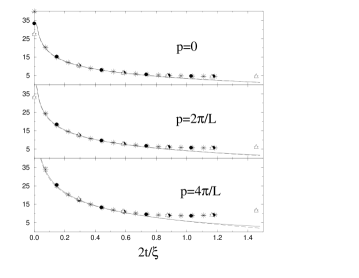
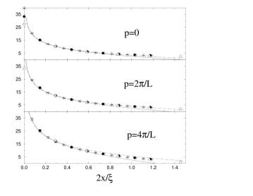
The one-particle matrix elements of the product on the l.h.s. of Eq. (4.4.7) can be obtained from the function $G^{(0)}(t,x;\overline{p},\overline{q};2t_{s})$, see Eq. (4.4.13). Indeed we know that

$$\langle\overline{p},a|\mbox{\boldmath$\sigma$}_{t,x}\cdot\mbox{\boldmath$\sigma$}_{-t,-x}|\overline{q},a\rangle=\sqrt{4\omega(\overline{p})\omega(\overline{q})}\lim_{t_{s}\to\infty}\widehat{G}^{(0)}(t,x;\overline{p},\overline{q};2t_{s})\,.$$ (4.4.52)

We computed $\widehat{G}^{(0)}(t,x;\overline{p},\overline{p};2t_{s})$ for different values of $t_{s}$ (with $t_{s}\mathrel{\hbox to0.0pt{\lower 3.0pt\hbox{$\mathchar 536\relax$}\hss}\raise 2.0pt\hbox{$\mathchar 318\relax$}}\xi_{\rm exp}$, see Sec. 4.4.1) and verified it to be independent of $t_{s}$ in that range. This is compatible with the findings of Secs. 4.4.2 and 4.4.5: the on-shell limit for one-particle states is reached, with a good approximation, at time separations $t_{s}\mathrel{\hbox to0.0pt{\lower 3.0pt\hbox{$\mathchar 536\relax$}\hss}\raise 2.0pt\hbox{$\mathchar 318\relax$}}\xi_{\rm exp}$. We evaluated the limit on the r.h.s. of Eq. (4.4.52) using the lowest value of $t_{s}$ in the range considered in our Monte Carlo calculations. In particular we use $t_{s}=8$ on lattice (A), $t_{s}=16$ on lattice (B) and $t_{s}=30$ on lattice (C). The same procedure will be applied in the next Sections. In Fig. 4.9 we compare the numerical results obtained in this manner with the OPE fit.

The parametrization in Eqs. (4.4.47), (4.4.48), and the OPE (4.4.7) imply the following fitting form:

$$2\sqrt{\overline{p}^{2}+m^{2}}{\rm Re}\,\widehat{G}^{(0)}(t,x;\overline{p},\overline{p};2t_{s}) = 2\sqrt{\overline{p}^{2}+m^{2}}L{\cal F}_{RGI,0}^{(1)}(\overline{g}_{\zeta}(r);\zeta){\cal Z}^{\prime}+$$

$$+\widehat{\cal F}^{(1)}_{RGI,1}(\overline{g}_{\zeta}(r);\zeta)(m^{2}+2\overline{p}^{2})(x^{2}-t^{2}){\cal T}+\widehat{\cal F}^{(1)}_{RGI,2}(\overline{g}_{\zeta}(r);\zeta)m^{2}r^{2}{\cal E}\,.$$

The renormalized parameters ${\cal T}_{R}$ and ${\cal E}_{R}$ are related to their unrenormalized counterparts ${\cal T}$ and ${\cal E}$ through the renormalization of the fields $\sigma$ on te l.h.s. of Eq. (4.4.7). In particular we can estimate ${\cal T}_{R}$ and ${\cal E}_{R}$ using, respectively, $Z_{L}^{-1}{\cal T}$ and $Z_{L}^{-1}{\cal E}$. The parameter ${\cal Z}^{\prime}$ give access to the field-renormalization constant $Z_{L}$, analogously to the parameter ${\cal Z}$ in Sec. 4.4.4.

In Fig. 4.9 we plot $2\sqrt{\overline{p}^{2}+m^{2}}Z_{L}^{-1}\widehat{G}^{(0)}(t,x;\overline{p};2t_{s})$ on lattice (A) ($t_{s}=8$), (B) ($t_{s}=16$) and (C) ($t_{s}=30$), versus the separation between $\sigma(x)$ and $\sigma(-x)$ in physical units: $2r/\xi_{\rm exp}$. This function should have a finite $a\to 0$ limit (at $2r/\xi_{\rm exp}$ fixed). We used the values of $Z_{L}$ estimated with the OPE method in Sec. 4.4.4, see Tab. 4.3, second column, and the results for $\xi_{\rm exp}$ of the previous Chapter, see Eq. (3.3.4). The results obtained on lattices (A), (B) and (C) collapse except for $r=0$, as expected. This fact indicates that we are in the scaling regime.

The best fitting curves shown in Fig. 4.9 have been obtained on lattice (C). We used a fitting window $\rho\leq r\leq R$, with $\rho=0.5$ and $R=7.5$. The fit is quite good for $2r/\xi\mathrel{\hbox to0.0pt{\lower 3.0pt\hbox{$\mathchar 536\relax$}\hss}\raise 2.0pt\hbox{$\mathchar 316\relax$}}0.6$. We used the fitting form (4.4.7) both with ${\cal Z}^{\prime}$, ${\cal E}$, ${\cal T}$ free, and with ${\cal Z}^{\prime}$ free and ${\cal E}={\cal T}=0$ (i.e. in this case we kept only the leading term of Eq. (4.4.7)). The difference between the two fitting procedure is hardly visible. The reason is that the first term in Eq. (4.4.7) is of order $L/\xi$ with respect to the other ones in the thermodynamic limit ($L\to\infty$ at fixed $g_{L}$).

Figure 4.10: The best fitting parameters $\widehat{\cal Z}^{\prime}(\rho,R)$ (graphs (A) and (A’)), $\widehat{\cal T}(\rho,R)$ (graph (B)) and ${\cal E}(\rho,R)$ (graph (C)) on lattice (B). Different symbols refer to different external momenta: $\overline{p}=0$ (empty circles) or $\overline{p}=2\pi/L$ (filled squares). The continuous horizontal lines in graphs (A), (A’) and (B) correspond to the prediction ${\cal Z^{\prime}}=Z_{L}$, ${\cal T}=Z_{L}$, with $Z_{L}\approx 0.559$ as estimated in Tab. 4.3.

Figure 4.11: As in Fig. 4.10 on lattice (C).

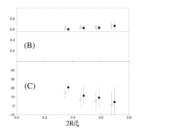
In Figs. 4.10 and 4.11 we study the dependence of the fit parameters upon $R$. Our aim is to understand whether a window for asymptotic scaling exists. We plot the best fitting values obtained with $\zeta e^{\gamma}=1$ together with the statistical and systematic uncertainties. For sake of clarity we limit ourselves to showing the results obtained with $\overline{p}=0,2\pi/L$ (the results for $\overline{p}=4\pi/L$ have larger statistical errors). In graphs (A), (B), (C) we used the fitting form (4.4.32) including power corrections. In (A’) we kept only the leading term of Eq. (4.4.32), i.e. ${\cal Z}^{\prime}$.

The remarks formulated in Sec. 4.4.4 can be repeated here. Statistical errors on our numerical data are, also in this case, quite small. Systematic errors on the leading operator are strongly reduced if power-correction terms are included in the fitting form. Nevertheless, as we already discussed in Sec. 4.4.4, this is a somewhat “spurious” effect.

4.4.8 OPE in the Antisymmetric Sector

We consider now the antisymmetric product of two elementary fields at short distances.

We start by rewriting the form of the OPE in terms of RGI operators, cf. Eq. (4.2.3):

$$\sigma^{[a}_{RGI}(x)\sigma^{b]}_{RGI}(-x) = -2x_{\mu}{\cal F}^{(1)}_{RGI}(\overline{g}_{\zeta}(r);\zeta)\,j^{ab}_{\mu}(0)\,,$$ (4.4.54)

where we neglected $O(r^{3})$ terms. Notice that the Noether current $j^{ab}_{\mu}$ is RGI (this happens for any regularization and any renormalization scheme). As a consequence we did not add any subscript to it. The Wilson coefficient is easily obtained from Eq. (4.2) using the formulae of Sec. 2.7:

$${\cal F}^{(1)}_{RGI}(\overline{g};1) = g^{-1/(N-2)}\left\{1+\frac{N-1}{2\pi(N-2)}\overline{g}-\frac{2N^{3}-13N^{2}+24N-14}{16\pi^{2}(N-2)^{2}}\overline{g}^{2}\right\}\,.$$

Before continuing we remark that the $O(N)$ symmetry fixes the normalization of the Noether current. This can be seen by considering the $O(N)$ charges $Q^{ab}$, and requiring that $Q^{ab}$ generates the $O(N)$ transformations:

$$Q^{ab}|\overline{p},c\rangle=\delta^{bc}|\overline{p},a\rangle-\delta^{ac}|\overline{p},b\rangle\,,\quad Q^{ab}\equiv\int_{-\infty}^{+\infty}\!\!\!dx\;j^{ab}_{0}(t,x)\,.$$ (4.4.56)

Using Lorentz invariance and the above condition we have:

$$\frac{1}{N}\sum_{a,b}\langle\overline{p},a|j^{ab}_{\mu}|\overline{p},b\rangle=-2ip_{\mu}(N-1)\,.$$ (4.4.57)

This identity allows a tight check of the expansion (4.4.54).

The OPE (4.4.54) is quite different from the other examples studied in this Chapter. Since there exists no dimension-zero antisymmetric operator, the leading term is of order $O(r|\log r|^{p})$. In the other cases we have a much weaker $r$ dependence: $O(|\log r|^{p})$.

Figure 4.12: Monte Carlo results and OPE fit for the product of fields in the antisymmetric sector. We report $2\sqrt{\overline{p}^{2}+m^{2}}Z_{L}^{-1}\widehat{G}^{(1)}(t,x;\overline{p};2t_{s})$ on lattices (A) (empty triangles, $\triangle$), (B) (filled circles, $\bullet$) and (C) (stars, $\ast$). We consider $x=0$, $t\neq 0$ on the left, and $x=t=r/\sqrt{2}$ on the right. The continuous curves are fits to the leading term of the OPE.

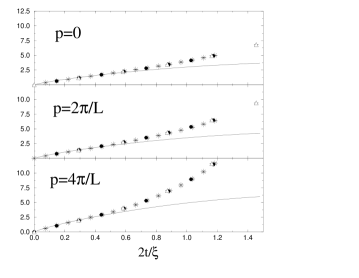
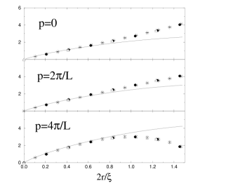
The one-particle matrix elements have been extracted as explained in the previous Subsection, see Eq. (4.4.52). We rewrite here the relevant equation in order to specify the correct normalization

$$\sum_{a,b}\langle\overline{p},a|\sigma^{[a}_{t,x}\sigma^{b]}_{-t,-x}|\overline{q},b\rangle=N\sqrt{4\omega(\overline{p})\omega(\overline{q})}\lim_{t_{s}\to\infty}\widehat{G}^{(1)}(t,x;\overline{p},\overline{q};2t_{s})\,.$$ (4.4.58)

In Fig. 4.12 we show the numerical results for the $\langle\overline{p}|\cdot|\overline{p}\rangle$ matrix elements. We plot the function $2\sqrt{\overline{p}^{2}+m^{2}}Z_{L}^{-1}{\rm Re}\,\widehat{G}^{(1)}(t,x;\overline{p},\overline{p};2t_{s})$ along the directions $(t,x)=(t,0)$ and $(t,x)=(t,t)$. In this case a plot along the direction $(t,x)=(0,x)$ would be trivial, since ${\rm Re}\,\widehat{G}^{(1)}(0,x;\overline{p},\overline{p};2t_{s})=0$. The non-perturbative results of Sec. 4.4.4, see Tab. 4.3, have been used to estimate $Z_{L}$.

The OPE (4.4.54) and the identity (4.4.57) imply the following fitting form

$$2\sqrt{\overline{p}^{2}+m^{2}}{\rm Re}\,\widehat{G}^{(1)}(t,x;\overline{p},\overline{p};2t_{s})=2\sqrt{\overline{p}^{2}+m^{2}}(N-1){\cal F}^{(1)}(\overline{g}_{\zeta}(r);\zeta)\,t\,{\cal Z}^{\prime\prime}\,,$$ (4.4.59)

where ${\cal Z}^{\prime\prime}$ is an estimate of the field-renormalization constant (analogously to ${\cal Z}$ in Sec. 4.4.4, and ${\cal Z}^{\prime}$ in Sec. 4.4.7). In Fig. 4.12 we show the best fitting curves of the form (4.4.59), as determined on lattice (C). We used a fitting window $\rho\leq r\leq R$ with $\rho=0.5$ and $R=7.5$. The collapse of the data obtained on different lattices indicates that scaling is well verified by our numerical results for $\widehat{G}^{(1)}$. Moreover, the fitting curves are in good agreement with numerical data up to $2r/\xi\sim 0.5$.

Figure 4.13: The best fitting parameter $\widehat{\cal Z}^{\prime\prime}(\rho,R)$ on lattice (B) (graphs (A) and (A’)), and lattice (C) (graphs (B) and (B’)). We use one-loop perturbation theory in graphs (A) and (B), and two-loop perturbation theory in (A’) and (B’). Different symbols refer to different external momenta: $\overline{p}=0$ (empty circles) or $\overline{p}=2\pi/L$ (filled squares). The horizontal lines correspond to the theoretical prediction ${\cal Z}^{\prime\prime}(\rho,R)=\widehat{\cal Z}^{*}$, see Tab. 4.3.

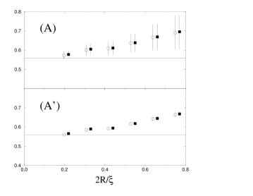
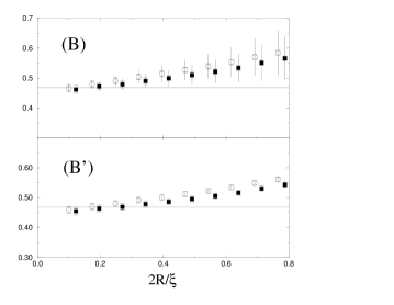
In Fig. 4.13 we study the $R$ dependence of the best fitting parameter $\widehat{\cal Z}^{\prime\prime}(\rho,R)$, keeping $\rho=0.5$ fixed. In graphs (A) and (B) we present the results obtained with the one-loop Wilson coefficient, which is given by dropping out the $O(\overline{g}^{2})$ term in Eq. (LABEL:WilsonAntiSymmetric). In graphs (A’) and (B’) we use the two-loop Wilson coefficient (LABEL:WilsonAntiSymmetric). The continuous lines refer to the field renormalization constant as computed in Sec. 4.4.4.

One-loop results, i.e. graphs (A) and (B), are almost flat within the systematic errors and agree with the prediction of Sec. 4.4.4 for the field-renormalization constant. Our estimate of the systematic errors seems to be quite good in this case.

$\widehat{\cal Z}^{\prime\prime}(\rho,R)$ $\widehat{\cal Z}^{*}$ $\overline{p}=0$ $\overline{p}=2\pi/L$ $\overline{p}=4\pi/L$ lattice (A) $0.791(2)[14]$ $0.787(1)[14]$ $0.783(4)[14]$ $0.67[1]$ lattice (B) $0.585(4)[4]$ $0.590(4)[4]$ $0.577(12)[4]$ $0.559[5]$ lattice (C) $0.480(10)[3]$ $0.469(11)[2]$ $0.484(26)[3]$ $0.468[3]$

Table 4.8: The field renormalization constant as computed from the numerical results in the antisymmetric sector with the fitting form (4.4.59). Notice that in this case we found no scaling window. We quote the best fitting parameters obtained with $R=2.5$ on lattices (A) and (B), and $R=3.5$ on lattice (C). For sake of comparison, we report in the fifth column the estimates of the field-renormalization constant obtained in Sec. 4.4.4, cf. Tab. 4.3.

Two-loop results, i.e. graphs (A’) and (B’) do not differ much from their one-loop counterparts, as far as the central value for $\widehat{\cal Z}^{\prime\prime}(\rho,R)$ (corresponding to $\zeta e^{\gamma}=1$) is concerned. However systematic errors are greatly reduced. They are much smaller than systematic errors obtained in the scalar or symmetric sectors with the same number of loops, at the same values of $R$. As a consequence the two-loop results for $\widehat{\cal Z}^{\prime\prime}(\rho,R)$ are no longer flat. Looking at Fig. 4.13, graphs (A’) and (B’), we cannot find any “scaling window”. Nevertheless, for small $R$, $\widehat{\cal Z}^{\prime\prime}(\rho,R)$ seems to converge to the field-renormalization constant computed in Sec. 4.4.4. In Tab. 4.8 we report the values of $\widehat{\cal Z}^{\prime\prime}(\rho,R)$ obtained with $R=2.5$ on lattices (A) and (B), and $R=3.5$ on lattice (C).

Figure 4.14: The best fitting parameters $\widehat{\cal Z}^{\prime\prime}(\rho,R)$ (graphs (A) and (A’)), $\widehat{\cal M}(\rho,R)$ (graph (B)) and $\widehat{\cal N}(\rho,R)$ (graph (C)) corresponding to the fitting form (4.4.60). These results have been obtained on lattice (C). We use one-loop perturbation theory for the leading Wilson coefficient in graphs (A), and two-loop perturbation theory in (A’), (B) and (C). Different symbols refer to different external momenta: $\overline{p}=0$ (empty circles) or $\overline{p}=2\pi/L$ (filled squares). The horizontal lines in (A) and (A’) correspond to the theoretical prediction ${\cal Z}^{\prime\prime}(\rho,R)=\widehat{\cal Z}^{*}$, see Tab. 4.3.

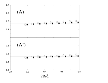
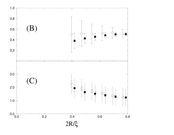
The discrepancy at larger values of $R$ can be attributed either to an imperfect evaluation of systematic errors (an unlucky numerical coincidence which makes them so small in this case), or to power-correction effects. In order to better understand the problem, we tried to fit the numerical data using the following “phenomenological” form:

$$2\sqrt{\overline{p}^{2}+m^{2}}{\rm Re}\,\widehat{G}^{(1)}(t,x;\overline{p},\overline{p};2t_{s}) = 2\sqrt{\overline{p}^{2}+m^{2}}(N-1){\cal F}^{(1)}(\overline{g}_{\zeta}(r);\zeta)\,t\,{\cal Z}^{\prime\prime}+$$ (4.4.60)

$$+(\overline{p}^{2}+m^{2}/4)\sqrt{\overline{p}^{2}+m^{2}}\,t(t^{2}-3x^{2})\,{\cal M}+$$

$$+m^{2}\sqrt{\overline{p}^{2}+m^{2}}\,t(t^{2}+x^{2})\,{\cal N}\,.$$

This fitting form is obtained as follows. We write down the $O(r^{3})$ terms of the OPE (4.4.54), and single out the Lorentz structure of the Wilson coefficients. The “reduced” Wilson coefficients depend logarithmically upon $r$ and are rotationally invariant. We make the crude approximation of neglecting this logarithmic $r$ dependence. Next, we single out the $\overline{p}$ dependence of the $\langle\overline{p}|\cdot|\overline{p}\rangle$ matrix elements of the composite operators of dimension 3. The $\overline{p}$ dependence can be easily deduced by using the space-time symmetries. It depends uniquely upon the spin of the composite operator. The result of this procedure has the form 4.4.60.

The functions multiplying ${\cal M}$ and ${\cal N}$ have the same dimension and Lorentz structure as the Wilson coefficients of the next-to-leading terms in the OPE (4.4.54). The parameters ${\cal M}$ and ${\cal N}$ correspond, respectively, to dimension 3, spin 3 operators, and to dimension 3, spin 1 operators.

Equation (4.4.60) can be considered, for what concerns power corrections, as a “naive” (i.e. not RG improved) tree-level approximation. Since power corrections in Eq. (4.4.60) do not have the correct $r\to 0$ limit, the parameters ${\cal M}$ and ${\cal N}$ do not give access to well-defined matrix elements. Anyway, by adopting the fitting form (4.4.60), we gain some insight into the role of power corrections for the determination of ${\cal Z}^{\prime\prime}$.

The results obtained on lattice (C) are shown in Fig. 4.14. Notice that $\widehat{\cal Z}^{\prime\prime}(\rho,R)$ is much flatter than in Fig. 4.14. The estimation at small $R$ does not change much and is compatible with the one of Sec. 4.4.4. For instance at $R=3.5$ on lattice (C) we get $\widehat{\cal Z}^{\prime\prime}(\rho,R)=0.459(11)[2]$ (here we quote the result at $\overline{p}=0$), cf. Tab. 4.8.

4.4.9 OPE in the Symmetric Sector

Our last example concerns the symmetric traceless product of two elementary fields at short distances.

We shall keep track of the $O(r^{2})$ power corrections in the OPE. As a consequence, we must take care of the non-trivial mixing between dimension-2 symmetric traceless operators, see Sec. 2.3.3. For this task, it is convenient to adopt the basis of operators with definite spin, see Eqs. (2.4.25)–(2.4.31).

For sake of clarity we shall restrict ourselves to the case of on-shell external states of equal total momentum. This allows two simplifications. We can eliminate the operators $Q^{R(6)}$ and $Q^{R(7)}$ since they vanish on shell, see Eqs. (2.3.60) and (2.3.60). We can eliminate $Q^{R(4)}_{\mu\nu}$ and $Q^{R(5)}$, which are total space-time derivatives. With these assumptions we get from Eq. (4.2.4)

$$\frac{1}{2}\sigma^{\{a}_{RGI}(x)\sigma^{b\}}_{RGI}(-x)-\frac{\delta^{ab}}{N}\mbox{\boldmath$\sigma$}_{RGI}(x)\cdot\mbox{\boldmath$\sigma$}_{RGI}(-x) = {\cal F}^{(2)}_{RGI,0}(\overline{g}_{\zeta}(r);\zeta)\,\left[S_{0}^{ab}\right]_{RGI}+$$ (4.4.61)

$$+\sum_{i=1}^{3}{\cal F}^{(2)}_{RGI,i}(\overline{g}_{\zeta}(r);\zeta)x^{\mu}x^{\nu}\left[Q^{(i)}_{\mu\nu}\right]_{RGI}\,,$$

where we used, once more, renormalization-group invariant operators. The coefficients ${\cal F}^{(2)}_{RGI,i}(\overline{g};1)$ for $i=1,2,3$ are given in Eqs. (4.3.48)-(4.3.50) for $N=3$. The coefficient of the leading term can be calculated from Eq. (4.2.11):

$${\cal F}^{(2)}_{RGI,0}(\overline{g};1)=\overline{g}^{1/(N-2)}\left[1-\frac{1}{2\pi(N-2)}\overline{g}+\frac{N^{2}-4N+6}{16\pi^{2}(N-2)^{2}}\overline{g}^{2}\right]\,.$$ (4.4.62)

We shall be interested in the $\langle\overline{p}|\cdot|\overline{p}\rangle$ matrix elements of Eq. (4.4.61). Analogously to Sec. 4.4.7, space-time symmetries constrain the matrix elements of the composite operators on the right-hand side of Eq. (4.4.61). Here we adopt the following parametrization:

$$\frac{1}{N}\sum_{ab}\langle\overline{p},a|\left[S_{0}^{ab}\right]_{RGI}|\overline{p},b\rangle = {\cal A}_{R}\,,$$ (4.4.63)

$$\frac{1}{N}\sum_{ab}\langle\overline{p},a|\left[Q^{(1)ab}_{\mu\nu}\right]_{RGI}|\overline{p},b\rangle = {\cal B}_{R}\,(p_{\mu}p_{\nu}-\frac{1}{2}\delta_{\mu\nu}p^{2})\,,$$ (4.4.64)

$$\frac{1}{N}\sum_{ab}\langle\overline{p},a|\left[Q^{(3)ab}_{\mu\nu}\right]_{RGI}|\overline{p},b\rangle = {\cal C}_{R}\,(p_{\mu}p_{\nu}-\frac{1}{2}\delta_{\mu\nu}p^{2})\,,$$ (4.4.65)

$$\frac{1}{N}\sum_{ab}\langle\overline{p},a|\left[Q^{(2)ab}_{\mu\nu}\right]_{RGI}|\overline{p},b\rangle = {\cal D}_{R}\,p^{2}\delta_{\mu\nu}\,.$$ (4.4.66)

The parameters ${\cal A}_{R},\dots,{\cal D}_{R}$ are real numbers and do not depend upon the external momentum $\overline{p}$.

Let us make some remarks concerning the expansion (4.4.61). The operator $Q^{(2)}_{\mu\nu}=Q^{(2)}\delta_{\mu\nu}$ is a higher-twist operator and mixes under renormalization with the dimension-zero operator $S^{ab}_{0}$. The warnings expressed in Sec. 4.1.2 apply also to this case.

Let us now consider the operators $Q^{(1)}_{\mu\nu}$ and $Q^{(3)}_{\mu\nu}$. Since their canonical dimension is equal to their spin (dimension$=$spin$=2$), they are leading twists. As a consequence, they can be determined unambiguously from the expansion (4.4.61). This can be done analogously to what we explained in Sec. 4.4.7 for $\widehat{T}_{\mu\nu}$, cf. Eq. (4.4.49).

There is, however, a practical difficulty in the determination of $Q^{(1)}_{\mu\nu}$ and $Q^{(3)}_{\mu\nu}$. For sake of clarity we refer to the case $N=3$. In this case ${\cal F}_{RGI,3}^{(2)}(\overline{g};1)$ (which is of order $\overline{g}^{2}$) is strongly suppressed with respect to ${\cal F}_{RGI,1}^{(2)}(\overline{g};1)$ (of order 1). In order to disentangle the two contributions in Eq. (4.4.61), we should compute ${\cal F}_{RGI,1}^{(2)}(\overline{g};1)$ at least to order $\overline{g}^{2}$. Since we have computed ${\cal F}_{RGI,1}^{(2)}$ and ${\cal F}_{RGI,3}^{(2)}$ to one-loop order, we do not expect to obtain a good determination of $Q^{(3)}_{\mu\nu}$. The best fitting ${\cal C}$ (see Eq. (4.4.65)) will mimic the higher-loop contributions in ${\cal F}_{RGI,1}^{(2)}(\overline{g};1)$.

This difficulty is however quite different from the one described in Sec. 4.1.2. In the present case it would be “sufficient” to push forward the perturbative calculation of ${\cal F}_{RGI,1}^{(2)}(\overline{g};1)$, and to perform numerical simulations at large enough correlation lengths, in order to solve the problem.

Figure 4.15: Monte Carlo results and OPE fit for the product of fields in the symmetric sector. We report $4\sqrt{\overline{p}^{2}+m^{2}}Z_{L}^{-1}\widehat{G}^{(2)}(t,x;\overline{p};2t_{s})$ on lattices (A) (empty triangles, $\triangle$), (B) (filled circles, $\bullet$) and (C) (stars, $\ast$). We consider $x=0$, $t\neq 0$ on the left, and $x\neq 0$, $t=0$ on the right. The dashed curves are obtained with the leading term of the OPE, the continuous curves include power corrections.

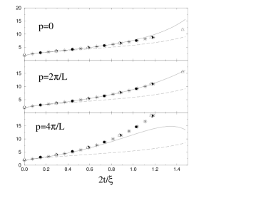
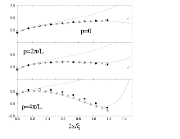
One-particle matrix elements have been extracted from the function $\widehat{G}^{(2)}(t,x;\overline{p},\overline{q};2t_{s})$ as explained in Secs. 4.4.7 and 4.4.8. The relation between one-particle matrix elements and the $t_{s}\to\infty$ limit of $\widehat{G}^{(2)}(t,x;\overline{p},\overline{q};2t_{s})$ is given by:

$$\frac{1}{2}\sum_{ab}\langle\overline{p},a|\sigma^{\{a}_{t,x}\sigma^{b\}}_{-t,-x}-\frac{2\delta^{ab}}{N}\mbox{\boldmath$\sigma$}_{t,x}\cdot\mbox{\boldmath$\sigma$}_{-t,-x}|\overline{q},b\rangle=N\sqrt{4\omega(\overline{p})\omega(\overline{q})}\lim_{t_{s}\to\infty}\widehat{G}^{(2)}(t,x;\overline{p},\overline{q};2t_{s})\,.$$

(4.4.67)

In Fig. 4.15 we present the results of this computation. We plot the function $4\sqrt{\overline{p}^{2}+m^{2}}Z_{L}^{-1}{\rm Re}\,\widehat{G}^{(2)}(t,x;\overline{p},\overline{p};2t_{s})$ along the directions $(t,x)=(t,0)$ and $(t,x)=(0,x)$. We used the non-perturbative estimates of $Z_{L}$ given in Sec. 4.4.4, see Tab. 4.3. Together with the numerical data we show the best fitting curves. The form of the fit is easily obtained from Eqs. (4.4.61) and (4.4.63)–(4.4.66):

$$2\sqrt{\overline{p}^{2}+m^{2}}\,{\rm Re}\,\widehat{G}^{(2)}(t,x;\overline{p},\overline{p};2t_{s}) = {\cal F}^{(2)}_{RGI,0}(\overline{g}_{\zeta}(r);\zeta){\cal A}-{\cal F}^{(2)}_{RGI,2}(\overline{g}_{\zeta}(r);\zeta)m^{2}r^{2}{\cal D}+$$

$$+{\cal F}^{(2)}_{RGI,1}(\overline{g}_{\zeta}(r);\zeta)(m^{2}/2+\overline{p}^{2})(x^{2}-t^{2}){\cal B}+$$

$$+{\cal F}^{(2)}_{RGI,3}(\overline{g}_{\zeta}(r);\zeta)(m^{2}/2+\overline{p}^{2})(x^{2}-t^{2}){\cal C}\,.$$

The curves in Fig. 4.15 are the best fitting curves obtained on lattice (C). For these curves we use a fitting window $\rho\leq r\leq R$, with $\rho=0.5$ and $R=8.5$. As usual we try two types of fit: with (continuous line) and without (dashed line) power corrections.

The fitting form which includes power corrections (i.e. the parameters ${\cal B}$, ${\cal C}$, ${\cal D}$, see Eq. (4.4.9)) describes very well the numerical data for $2r/\xi_{\rm exp}\mathrel{\hbox to0.0pt{\lower 3.0pt\hbox{$\mathchar 536\relax$}\hss}\raise 2.0pt\hbox{$\mathchar 316\relax$}}1$. At distances $2r/\xi_{\rm exp}\approx 1$ we expect both the OPE and the perturbative expansion to break down.

The fit without power corrections (which amounts to dropping the parameters ${\cal B}$, ${\cal C}$ and ${\cal D}$ in Eq. (4.4.9)) correctly captures the small-$r$ behaviour of $\widehat{G}^{(2)}(t,x;$ $\overline{p},\overline{p};2t_{s})$. The deviations from the numerical data become quite large as soon as $2r/\xi_{\rm exp}\mathrel{\hbox to0.0pt{\lower 3.0pt\hbox{$\mathchar 536\relax$}\hss}\raise 2.0pt\hbox{$\mathchar 318\relax$}}0.3$ and depend upon the direction. These deviations are mainly due to spin $2$ operators in the OPE (4.4.61). Such terms are effectively averaged out when considering a rotationally invariant fitting form (like the one without power corrections). As a consequence the best fitting value of ${\cal A}$ does not change very much whether or not power correction terms are included in the fitting form.

Figure 4.16: The renormalized fitting parameters $\widehat{\cal A}_{R}(\rho,R)$ (graphs (A) and (A’)), $\widehat{\cal B}_{R}(\rho,R)$ (graph (B)), $\widehat{\cal C}_{R}(\rho,R)$ (graph (C)), and $\widehat{\cal D}_{R}(\rho,R)$ (graph (D)). Empty circles and filled squares refer, respectively, to $\overline{p}=0$ and $\overline{p}=2\pi/L$. The dashed lines in graphs (A) and (A’) (${\cal A}_{R}=1.3$), and in graph (B) (${\cal B}_{R}=5$) are a guide for the eye. These data refer to lattice (B).

Figure 4.17: The same as in Fig. 4.16 on lattice (C).

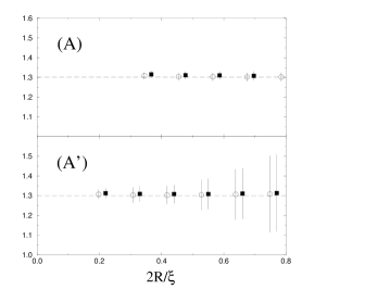
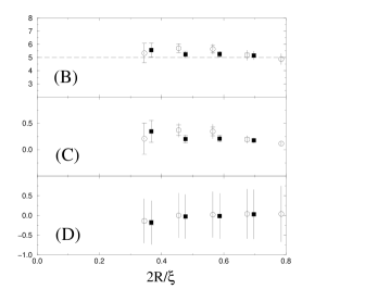
In Figs. 4.16 and 4.17 we report the best fitting parameters as a function of the fitting window $\rho\leq r\leq R$. We keep $\rho=0.5$ fixed and vary $R$. The kinematic scaling (independence of the parameters upon $\overline{p}$) is verified within the statistical error. The only exception is given by parameter ${\cal A}$ on lattice (A). However this effect is very small (about the $1.0\div 1.5\%$) and can be ascribed to scaling corrections.

In the majority of the cases, statistical errors on the fitting parameters are by far smaller than systematic ones. There are some exceptions to this rule. Consider for instance parameters ${\cal B}$ and ${\cal C}$ on lattices (B) and (C), see Figs. 4.16 and 4.17, graphs (B) and (C). As $R\to 0$ statistical errors become larger than systematic ones. The reason of this fact is quite simple. At small $R$ the contribution of power corrections vanishes. The corresponding fitting parameters are fixed essentially by statistical fluctuations.

Let us now come to the cautious remarks concerning the evaluation of $Q^{(2)}_{\mu\nu}$ and $Q^{(3)}_{\mu\nu}$ (i.e., respectively, the parameters ${\cal D}$ and ${\cal C}$) formulated at the beginning of this Section.

It is clear from Figs. 4.16 and 4.17, graphs (D), that any sound estimate of ${\cal D}$ is hopeless. The central value $\widehat{\cal D}(r,R)$ (obtained with $\zeta e^{\gamma}=1$) is approximatively zero (namely it is of order $10^{-1}\div 10^{-2}$), with systematic errors of order 1. This is true on all the lattices and for all the values of $R$ considered. Let us suppose to repeat the calculation by fixing a particular perturbative truncation of the Wilson coefficients. We shall obtain, in general, values of $\widehat{\cal D}(\rho,R)$ of order one. Nevertheless the results will depend strongly upon the chosen truncation. In our approach we can look at $\widehat{\cal D}_{\zeta}(\rho,R)$, which depends depends upon $\zeta$. As $\zeta$ is varied the neglected higher-loops contributions to ${\cal F}^{(2)}_{RGI,0}(\overline{g}_{\zeta}(r);\zeta)$ vary. The value of $\widehat{\cal D}_{\zeta}(\rho,R)$ determined by the fit mimics these higher-order terms.

A subtle point in the computation of ${\cal D}$ is the following. Suppose to choose a particular value of $R/\xi_{\rm exp}$ and a particular perturbative truncation of the Wilson coefficients, i.e., in our approach, a particular value of $\zeta$. Then compute $\widehat{\cal D}_{\zeta}(\rho,R)$ for several values of the bare coupling $g_{L}$. This amounts to choosing several values of the lattice spacing. It is not unlikely that the matrix elements of $Q^{(2)}_{\mu\nu}$ obtained in this way will have (roughly) the correct scaling with the lattice spacing. In other words one obtains $\widehat{\cal D}_{\zeta}(\rho,R)$ which is approximatively independent of $g_{L}$, instead of having a power-like dependence upon the lattice spacing. For example on lattices (A), (B) and (C) at $\zeta=1$ and $R/\xi_{\rm exp}=0.367$ we get, respectively, $\widehat{\cal D}=-0.308(4)$, $-0.238(5)$ and $-0.189(17)$ (the quoted values refer to $\overline{p}=0$ and the corresponding statistical error). This fact could led to the conclusion that a genuine physical (continuum) quantity has been estimated despite the theoretical warnings. The analysis in the previous paragraphs shows, however, that this estimate is unreliable.

Let us now consider the parameter ${\cal C}$, i.e. the operator $Q^{(3)}_{\mu\nu}$, whose $R$ dependence is shown in Figs. 4.16, 4.17, graphs (C). In the general discussion above, we stressed that, for a sound estimate of ${\cal C}$, a two-loop calculation of the Wilson coefficient ${\cal F}^{(2)}_{RGI,1}$ is needed. Here, we shall “guess” the two-loop result. This will provide us with an “instructive” estimate of ${\cal C}$.

From Tab. 4.1 we learn that (if $\zeta e^{\gamma}=1$ and $N=3$) one-loop coefficients are of order $10^{-1}$, while two-loop coefficients are of order $10^{-2}$. Let us suppose the same to be true for the unknown two-loop coefficient of ${\cal F}^{(2)}_{RGI,1}$. We can look at the values of $\widehat{\cal C}(\rho,R)$ presented in Figs. 4.16 and 4.17, graphs (C), as the sum of two contributions: the genuine matrix element of $Q^{(3)}_{\mu\nu}$, and a spurious contribution coming from the two-loop term of ${\cal F}^{(2)}_{RGI,1}$. Using the value of ${\cal B}$ given below (${\cal B}\approx 3$), we can estimate the spurious contribution to be about $10^{-2}\div 10^{-1}$. We can now subtract this contribution from the best fitting values $\widehat{\cal C}(\rho,R)$ reported in Figs. 4.16, 4.17, graphs (C). We obtain ${\cal C}$ of order $10^{-1}$: a conservative estimate is then ${\cal C}\mathrel{\hbox to0.0pt{\lower 3.0pt\hbox{$\mathchar 536\relax$}\hss}\raise 2.0pt\hbox{$\mathchar 316\relax$}}1$. It is interesting to notice that the systematic errors in Figs. 4.16, 4.17, graphs (C) are about $0.2\div 0.5$ for intermediate values of $2R/\xi$. They correctly signal the effects due to the perturbative truncation of the Wilson coefficients.

	$\widehat{\cal A}^{*}$			$\widehat{\cal B}*$
	$\overline{p}=0$	$\overline{p}=2\pi/L$	$\overline{p}=4\pi/L$	$\overline{p}=0$	$\overline{p}=2\pi/L$	$\overline{p}=4\pi/L$
lattice (A)	$0.91(0)[11]$	$0.90(0)[11]$	$0.90(1)[11]$	$3.14(3)[29]$	$3.16(2)[31]$	$3.26(5)[36]$
lattice (B)	$0.73(0)[2]$	$0.73(0)[2]$	$0.74(1)[2]$	$2.58(4)[35]$	$2.53(4)[36]$	$2.63(6)[37]$
lattice (C)	$0.60(1)[1]$	$0.61(1)[1]$	$0.57(4)[1]$	$2.1(1)[2]$	$2.2(1)[3]$	$2.4(2)[4]$

Table 4.9: The unrenormalized OPE estimates for the matrix elements of $\left[S_{0}\right]_{RGI}$ and $[Q^{(3)}_{\mu\nu}]_{RGI}$.

We shall now consider the leading operator $S_{0}$ (and the corresponding parameter ${\cal A}$). In Figs. 4.16 and 4.17, graphs (A), we report the values of $\widehat{\cal A}(\rho,R)$ obtained with the fitting form (4.4.9). In the graphs (A’) of the same figures, we repeat the fit using only the leading term of the OPE, i.e. we drop out the terms ${\cal B}$, ${\cal C}$ and ${\cal D}$ in Eq. (4.4.9).

The results for $\widehat{\cal A}(\rho,R)$ obtained including power corrections, reported in graphs (A), are flat within statistical errors (approximatively $2\%$) as soon as $2R/\xi_{\rm exp}\mathrel{\hbox to0.0pt{\lower 3.0pt\hbox{$\mathchar 536\relax$}\hss}\raise 2.0pt\hbox{$\mathchar 316\relax$}}1$. The estimates obtained without power corrections , see graphs (A’), coincide with the previous ones within systematic errors. Systematic errors are strikingly different between graphs (A) and (A’). This phenomenon was already remarked in Sec. 4.4.4. Here we limit ourselves to underline a consequence of this fact. The systematic error on the final evaluation of the parameter ${\cal A}$ (i.e. on $\widehat{\cal A}^{*}$) strongly depends upon the lattice spacing, i.e. upon the bare coupling $g_{L}$. For instance if we fix $R=3.5$ and $\overline{p}=0$ we get ${\cal A}=0.91[37]$, $0.73[4]$ and $0.60[1]$ respectively on lattices (A), (B) and (C). Obviously systematic errors can be reduced on coarser lattices by taking smaller values of $R$, but one cannot reduce $R$ below the lattice spacing.

As we did in the previous Subsections, we estimate the systematic error from the fit without power corrections. Our final results for parameter ${\cal A}$ are given in Tab. 4.9. Here we used $R=2.5$ on lattices (A) and (B) while $R=3.5$ on lattice (C).

Finally we consider the evaluation of the parameter ${\cal B}$ (i.e. of the matrix element of $Q^{(3)}_{\mu\nu}$). Here we cannot apply the same strategy as for ${\cal A}$, that is taking smaller values of $R/\xi$ as $\xi$ gets larger (ideally $R/\xi\to 0$ and $R\to\infty$). As we explained above, if $R/\xi$ is small, the statistical error on ${\cal B}$ becomes large. We shall keep $R/\xi_{\rm exp}$ roughly fixed. Moreover $R/\xi_{\rm exp}$ must be taken in the perturbative regime. In Tab. 4.9 we present the corresponding estimates of ${\cal B}$ obtained with $R=3.5$, $7$ and $13.5$, respectively on lattices (A),(B) and (C).

$\widehat{\cal A}_{R}^{*}$ $\widehat{\cal B}_{R}^{*}$ lattice (A) $1.359(25)[157]$ $4.68(4)[44]$ lattice (B) $1.303(7)[39]$ $4.62(7)[63]$ lattice (C) $1.286(26)[24]$ $4.4(3)[4]$

Table 4.10: The renormalized fitting parameters corresponding to the matrix elements of $\left[S_{0}\right]_{RGI}$ and $[Q^{(3)}_{\mu\nu}]_{RGI}$.

We want to have an idea of the soundness of the systematic error bars quoted in Tab. 4.9. A possible check consists in looking at the results for the parameter ${\cal A}$ when the corresponding Wilson coefficient ${\cal F}^{(2)}_{RGI,0}(\overline{g}_{\zeta}(r);\zeta)$ is truncated to one-loop order. Using the fitting form (4.4.9) without power corrections, $\overline{p}=0$, and the same values of $R$ as the ones used for Tab. 4.9, we obtain ${\cal A}=0.95(0)[13]$, $0.75(0)[3]$ and $0.61(1)[2]$, respectively on lattices (A), (B) and (C).

Finally, in Tab. 4.10, we report the renormalized parameters corresponding to the matrix elements of $S_{0}$ and $Q^{(1)}_{\mu\nu}$ . The bare values are taken from the $\overline{p}=0$ columns of Tab. 4.9. They have been renormalized using the field renormalization constant computed in Sec. 4.4.4, cf. Tab. 4.3. The results for $S_{0}$ can be compared with the ones of Secs. 4.4.5 and 4.4.6, reported in the rightmost column of Tab. 4.7. We recall that in Secs. 4.4.5 and 4.4.6, we adopted a completely different method for the computation of the renormalized matrix elements of $S_{0}$. The two calculations agree very well, yielding a strong consistency check of the OPE method.

4.5 More Answers

The investigations described in this Chapter allow us to complete the partial conclusions of Sec. 3.4.

In this Chapter we considered short distance products of the form $\sigma(x)\sigma(y)$. As in the previous Chapter, the leading behaviour of this product was of the type $r^{0}$ (where $r=|x-y|$) in most of our examples (the only exception being the antisymmetric sector, see Sec. 4.4.8). It seems that such a situation is more favorable and we shall focus on it at first. Here we can make tighter statements than in Sec. 3.4, thanks to the smaller statistical errors (a fraction of percent) reached in this Chapter.

• Corrections to scaling determine the ultimate accuracy achievable at a given value of the bare coupling. The product of two elementary fields scales quite well, as long as the field operators are kept on different lattice sites. We were not able to reveal unambiguously corrections to scaling on these observables. We obtained some indications of scaling corrections (at the level of $1\%$) on lattice (A’), at $\xi_{\rm exp}=6.831(2)$.

• Higher-twist operators, i.e. operators which require power subtractions to be renormalized, cannot be determined from the OPE (at least in our simple approach). There are strong theoretical reasons pointing to this conclusion, see Sec. 4.1.2. The results obtained with the OPE method give a concrete support to these theoretical reasons.

• Leading-twist operator can be determined (at least in theory) from the OPE. They can be classified according to their canonical dimension. Those with the lowest dimension yield the leading contribution to the OPE. In all our examples there was a unique leading operator. We were able to determine its matrix elements with a few percent accuracy. We used (next-to-)²leading-log Wilson coefficients and products $\sigma(x)\sigma(y)$ at distances $r/\xi\sim 0.2\div 0.3$ ($r=|x-y|$).

• Higher-dimensional (leading-twist) operators appear as power corrections in the OPE. They can be determined from the OPE, but this task presents some technical difficulties. As the dimension of the operators increases, their mixings become more and more complicated. Moreover, at small distances (where perturbation theory is well behaved), their contribution to the OPE decreases quickly and statistical noise hides it.

• Including or not power corrections in the OPE fitting form seems not to be an important issue.

• As we already said in Sec. 3.4, the main problem is related to the need for asymptotic scaling. Usually asymptotic scaling is judged with respect statistical errors. If the perturbative prediction lies within statistical error bars, asymptotic scaling is considered to be reached. This point of view is not completely satisfactory. Among the other things it heavily depends upon the statistical accuracy. We proposed to estimate the convergence of perturbation theory by assigning a systematic error to it. There exists (to date) no proved good way to assign this systematic error. However, our “empirical” definition was in rough agreement with all our observations.

The example studied in Sec. 4.4.8, i.e. the antisymmetric product of two elementary fields, is somehow an exception to these remarks. This is perhaps related to the fact that the leading term of the OPE is, in this case, of order $r$, instead of $r^{0}$. In this case we were not able to find a scaling window without adding power corrections to the OPE fitting form. Taking care of power corrections at tree level allowed to improve the scaling behaviour. The final result was in good agreement with an alternative calculation. Nevertheless the situation is not fully satisfactory for what concerns this example.

Conclusions and Perspectives

Renormalization of lattice composite operators is a central problem for applications of lattice QCD. The structure of hadrons can be, for many purposes, encoded in matrix elements, which cannot be computed in perturbation theory. Lattice computations are a non-perturbative, widely applicable tool for such problems. Perturbation theory seems not to be the good method for translating the lattice results in the continuum language. This leads to the problem of designing well-chosen non-perturbative renormalization methods.

The authors of Ref. [32] proposed to define renormalized composite operators by “splitting” them into simpler operators (e.g., conserved currents). Operator Product Expansion must then be used for recovering the operator we were interested in. This is essentially an “infinite-volume scheme” (see Chapter 1) and has the disadvantage that many scales must be separated on the same lattice. However it has some advantages.

• Renormalized operators are obtained in a massless scheme without any extrapolation to the chiral limit.

• It is more direct: renormalization and computation of matrix elements are accomplished in the same step.

• A simpler approach to operator mixing is possible. In particular “lattice-induced” mixings can be disregarded since unrenormalized lattice operators are never used.

Moreover the idea itself is quite appealing. It is however far from obvious that it can applied in practice.

We completed a detailed feasibility study of this method on a simple two-dimensional model which can be simulated with very fast algorithms. We gave here a thorough account of this work. The main result is that the new method outlined above and in Section 1.4 really works. We refer to Secs. 3.4 and 4.5 for some technical highlights.

Here we recall the principal suggestions which come out from this work and could be of help in a QCD application of the new method:

• The model studied in this thesis is affected by $O(a^{2})$ lattice artifacts. The same type of corrections to scaling occurs in $O(a)$-improved QCD. We found the systematic errors due to these effects to be under control even on quite coarse lattices. The largest lattice artifacts occur in fact at contact points, and can be easily avoided in the OPE approach. On the coarsest lattice considered, the correlation length (inverse mass gap) was $\xi\approx 7a$.

• The principal source of systematic error is the perturbative truncation of the Wilson coefficients. We resummed the Wilson coefficients using RG up to next-to-next-to-leading-log order. We estimated the systematic error by varying the resummation procedure and the perturbative order. Moreover, we recomputed the same renormalized matrix elements using different approaches. The various estimates of the systematic error were roughly consistent. The achievable precision depends upon the lattice spacing, which control the shortest distance that can be reached on the lattice considered.

• Obviously, it is much simpler to estimate the leading operator of the OPE. The best situation occur when the corresponding Wilson coefficient behaves logarithmically in the short distance limit.

Let us conclude by listing a few lines for further investigation:

• In QCD chiral symmetries are broken both spontaneously, and “softly” by the quark-mass terms. These breakings manifest themselves as power corrections in the OPE. The role of these power corrections deserves some accurate investigation.

• What is the effect of improvement? One of the advantages of the method exposed here is that improvement of composite operators is straightforward. It would be interesting to study the efficiency of the method with an improved action and improved operators.

• The principal feature of the method studied in this thesis is that it allows to employ continuum symmetries, rather than lattice ones. This is an advantage both on the “standard” infinite-volume methods, and on the finite-volume ones. Therefore it would be very interesting to find a finite-volume version of the OPE method.

Bibliography

- [1] M. Testa, Non-Perturbative Renormalisation and Kaon Physics, Nucl. Phys. B (Proc. Suppl.) 63 (1998) 38, [hep-lat/9709044].
- [2] G. Buchalla, A. J. Buras, and M. E. Lautenbacher, Weak Decays Beyond Leading Logarithms, Rev. Mod. Phys. 68 (1996) 1125–1144, [hep-ph/9512380].
- [3] A. J. Buras, Weak Hamiltonian, CP Violation and Rare Decays, in Probing the Standard Model of Particle Interactions (F. David and R. Gupta, eds.), Elsevier Science B.V., 1998. hep-ph/9806471.
- [4] R. Petronzio, Structure Functions on the Lattice, Nucl. Phys. Proc. Suppl. 83-84 (2000) 136–139.
- [5] S. D. Joglekar and B. W. Lee, General Theory of Renormalization of Gauge Invariant Operators, Ann. Phys. 97 (1976) 160.
- [6] S. D. Joglekar, Local Operators Products in Gauge Theories. 1, Ann. Phys. 108 (1977) 233.
- [7] S. D. Joglekar, Local Operator Products in Gauge Theories. 2, Ann. Phys. 109 (1977) 210.
- [8] K. G. Wilson, Non-Lagrangian Models of Current Algebra, Phys. Rev. 179 (1969) 1499–1512.
- [9] W. Zimmerman in Lectures on Elementary Particles and Quantum Field Theory- 1970 Brandeis University Summer Institute in Theoretical Physics (S. Deser, H. Pendleton, and M. Grisaru, eds.), MIT Press, Cambridge, 1970.
- [10] M. Lüscher, R. Sommer, P. Weisz, and U. Wolff, A Precise Determination of the Running Coupling in the Yang-Mills Theory, Nucl. Phys. B413 (1994) 481–502, [hep-lat/9309005].
- [11] ALPHA Collaboration, S. Capitani, M. Lüscher, R. Sommer, and H. Wittig, Non-Perturbative Quark Mass Renormalization in Quenched Lattice QCD, Nucl. Phys. B544 (1999) 669, [hep-lat/9810063].
- [12] S. Weinberg, New Approach to the Renormalization Group, Phys. Rev. D8 (1973) 3497–3509.
- [13] M. Lüscher, S. Sint, R. Sommer, and W. P, Chiral Symmetry and O(a) Improvement in Lattice QCD, Nucl. Phys. B478 (1996) 365–400, [hep-lat/9605038].
- [14] G. Martinelli, C. Pittori, C. T. Sachrajda, M. Testa, and A. Vladikas, A General Method for Nonperturbative Renormalization of Lattice Operators, Nucl. Phys. B445 (1995) 81–108, [hep-lat/9411010].
- [15] A. Vladikas, Non-Perturbative Renormalization of Lattice Operators, Nucl. Phys. Proc. Suppl. 47 (1996) 84, [hep-lat/9510034].
- [16] G. C. Rossi, Non-Perturbative Renormalization in Lattice QCD, Nucl. Phys. Proc. Suppl. 53 (1997) 3–15, [hep-lat/9609038].
- [17] G. Martinelli, Hadronic Weak Interactions of Light Quarks, Nucl. Phys. B (Proc. Suppl.) 73 (1999) 58, [hep-lat/9810013].
- [18] V. Gimenez, L. Giusti, F. Rapuano, and M. Talevi, Non-Perturbative Renormalization of Quark Bilinears, Nucl. Phys. B531 (1998) 429, [hep-lat/9806006].
- [19] D. Becirevic, P. Boucaud, J. Leroy, V. Lubicz, G. Martinelli, and F. Mescia, Non-Perturbatively Renormalized Light-Quark Masses with the Alpha Action, Phys. Lett. B444 (1998) 401, [hep-lat/9807046].
- [20] M. Göckeler, R. Horsley, H. Oelrich, H. Perlt, D. Petters, P. E. L. Rakow, A. Schäfer, G. Schierholz, and A. Schiller, Nonperturbative Renormalisation of Composite Operators in Lattice QCD, Nucl. Phys. B544 (1999) 699, [hep-lat/9807044].
- [21] S. Capitani, M. Göckeler, R. Horsley, D. Petters, D. Pleiter, P. E. L. Rakow, G. Schierholz, A. Schiller, and P. Stephenson, Towards a Non-Perturbative Calculation of DIS Wilson Coefficients, Nucl. Phys. B (Proc. Suppl.) 73 (1999) 288, [hep-lat/9809171].
- [22] S. Capitani, M. Göckeler, R. Horsley, D. Petters, D. Pleiter, P. Rakow, and G. Schierholz, Higher-twist Corrections to Nucleon Structure Functions from Lattice QCD, Nucl. Phys. Proc. Suppl. 79 (1999) 173, [hep-ph/9906320].
- [23] K. Symanzik, Schrödinger representation and casimir effect in renormalizable quantum field theory, Nucl. Phys. B190 (1981) 1.
- [24] M. Lüscher, R. Narayanan, P. Weisz, and U. Wolff, The Schrödinger Functional: A Renormalizable Probe for Non-Abelian Gauge Theories, Nucl. Phys. B384 (1992) 168–228, [hep-lat/9207009].
- [25] M. Lüscher, R. Sommer, U. Wolff, and P. Weisz, Computation of the Running Coupling in the Yang-Mills Theory, Nucl. Phys. B389 (1993) 247–264, [hep-lat/9207010].
- [26] K. Jansen, C. Liu, M. Lüscher, H. Simma, S. Sint, R. Sommer, P. Weisz, and U. Wolff, Non-Perturbative Renormalization of Lattice QCD at all Scales, Phys. Lett. B372 (1996) 275–282, [hep-lat/9512009].
- [27] M. Lüscher, Advanced Lattice QCD, in Les Houches Summer School “Probing the Standard Model of Particle Interactions” (F. David and R. Gupta, eds.), 1998. hep-lat/9802029.
- [28] G. C. Rossi and M. Testa, The Structure of Yang-Mills Theories in the Temporal Gauge. 1. General Formulation, Nucl. Phys. B163 (1980) 109.
- [29] G. C. Rossi and M. Testa, The Structure of Yang-Mills Theories in the Temporal Gauge. 2. Perturbation Theory, Nucl. Phys. B176 (1980) 477.
- [30] G. C. Rossi and M. Testa, The Structure of Yang-Mills Theories in the Temporal Gauge. 3. The Instanton Sector, Nucl. Phys. B237 (1984) 442.
- [31] M. Guagnelli, K. Jansen, and R. Petronzio, Universal Continuum Limit of Non-Perturbative Lattice Non- Singlet Moment Evolution, Phys. Lett. B457 (1999) 153, [hep-lat/9901016].
- [32] C. Dawson, G. Martinelli, G. C. Rossi, C. T. Sachrajda, S. Sharpe, M. Talevi, and M. Testa, New Lattice Approaches to the Rule, Nucl. Phys. B514 (1998) 313, [hep-lat/9707009].
- [33] G. C. Rossi, Lattice Approach to the Rule, hep-lat/9811009.
- [34] N. D. Mermin and H. Wagner, Absence of Ferromagnetism or Antiferromagnetism in One- Dimensional or Two-Dimensional Isotropic Heisenberg Models, Phys. Rev. Lett. 17 (1966) 1133–1136.
- [35] S. Coleman, There are no Goldstone Bosons in Two-Dimensions, Commun. Math. Phys. 31 (1973) 259–264.
- [36] A. Jevicki, On the Ground State and Infrared Divergences of Goldstone Bosons in Two-Dimensions, Phys. Lett. B71 (1977) 327.
- [37] S. Elitzur, The Applicability of Perturbation Expansion to Two-Dimensional Goldstone Ststems, Nucl. Phys. B212 (1983) 501.
- [38] F. David, Cancellations of Infrared Divergences in the Two-Dimensional Nonlinear -Models, Commun. Math. Phys. 81 (1981) 149.
- [39] E. Brézin and J. Zinn-Justin, Renormalization of the Nonlinear -Model in Dimensions. Application to the Heisenberg Ferromagnets, Phys. Rev. Lett. 36 (1976) 691–694.
- [40] E. Brézin and J. Zinn-Justin, Spontaneous Breakdown of Continuous Symmetries near Two Dimensions, Phys. Rev. B14 (1976) 3110.
- [41] E. Brézin, J. Zinn-Justin, and J. C. L. Guillou, Renormalization of the Nonlinear -Model in Dimensions, Phys. Rev. D14 (1976) 2615.
- [42] S. Hikami, Three Loop Beta Functions of Nonlinear Models on Symmetric Spaces, Phys. Lett. 98B (1981) 208.
- [43] W. Bernreuther and F. J. Wegner, Four Loop Order Beta Function for Two-Dimensional Nonlinear Models, Phys. Rev. Lett. 57 (1986) 1383.
- [44] F. Wegner, Four Loop Order Beta Function of Nonlinear Models in Symmetric Spaces, Nucl. Phys. B316 (1989) 663.
- [45] E. Brézin, J. Zinn-Justin, and J. C. L. Guillou, Anomalous Dimensions of Composite Operators near Two Dimensions for Ferromagnets with Symmetry, Phys. Rev. B14 (1976) 4976.
- [46] J. Zinn-Justin, Quantum Field Theory and Critical Phenomena. Oxford University Press, Oxford, UK, 1996.
- [47] J. C. Collins, Renormalization. An Introduction to Renormalization, The Renormalization Group, And the Operator Product Expansion. Cambridge University Press, Cambridge, UK, 1984.
- [48] S. Caracciolo, A. Montanari, and A. Pelissetto, Testing the Efficiency of Different Improvement Programs, Nucl. Phys. B556 (1999) 295, [hep-lat/9812014].
- [49] P. Hasenfratz, Perturbation Theory and Zero Modes in Lattice -Models, Phys. Lett. B141 (1984) 385.
- [50] A. Patrascioiu and E. Seiler, Superinstantons and the Reliability of Perturbation Theory in NonAbelian Models, Phys. Rev. Lett. 74 (1995) 1920–1923, [hep-lat/9311019].
- [51] S. Caracciolo and A. Pelissetto, Four-Loop Perturbative Expansion for the Lattice -Vector Model, Nucl. Phys. B455 (1995) 619–647, [hep-lat/9510015].
- [52] D.-S. Shin, Correction to Four-Loop RG Functions in the Two-Dimensional Lattice Sigma-Model, Nucl. Phys. B546 (1999) 669, [hep-lat/9810025].
- [53] B. Allés, S. Caracciolo, A. Pelissetto, and M. Pepe, Four-Loop Contributions to Long-Distance Quantities in the Two-Dimensional Nonlinear -Model on a Square Lattice: Revised Numerical Estimates, Nucl. Phys. B562 (1999) 581–582, [hep-lat/9906014].
- [54] A. Buonanno, G. Cella, and G. Curci, Lattice Energy - Momentum tensor with Symanzik Improved Actions, Phys. Rev. D51 (1995) 4494, [hep-lat/9506008].
- [55] D.-S. Shin, A Determination of the Mass Gap in the Sigma-Model, Nucl. Phys. B496 (1997) 408, [hep-lat/9611006].
- [56] V. I. Arnold, Geometrical Methods in the Theory of Ordinary Differential Equations. Springer Verlag, New York, 1996.
- [57] W. Wasow, Asymptotic Expansions for Ordinary Differential Equations. Dover, New York, 1987.
- [58] P. Hasenfratz and F. Niedermayer, The Exact Mass Gap of the Model for Arbitrary in , Phys. Lett. B245 (1990) 529–532.
- [59] P. Hasenfratz, M. Maggiore, and F. Niedermayer, The Exact Mass Gap of the and Nonlinear Models in , Phys. Lett. B245 (1990) 522–528.
- [60] M. Lüscher, A New Method to Compute the Spectrum of Low-Lying States in Massless Asymptotically Free Field Theories, Phys.Lett. B118 (1982) 391.
- [61] M. Lüscher, P. Weisz, and U. Wolff, A Numerical Method to Compute the Running Coupling in Asymptotically Free Theories, Nucl. Phys. B359 (1991) 221–243.
- [62] S. Caracciolo, R. G. Edwards, A. Pelissetto, and A. D. Sokal, Asymptotic Scaling in the Two-Dimensional Model at Correlation Length , Phys. Rev. Lett. 75 (1995) 1891–1894, [hep-lat/9411009].
- [63] G. Parisi in Proc. XXth Conf. on High energy physics, Madison, WI, 1980.
- [64] G. Martinelli, G. Parisi, and R. Petronzio, Monte Carlo Simulations for the Two-Dimensional Nonlinear Sigma Model, Phys. Lett. B100 (1981) 485–488.
- [65] B. Allés, A. Buonanno, and G. Cella, Perturbation Theory Predictions and Monte Carlo Simulations for the 2D Nonlinear -Models, Nucl. Phys. B500 (1997) 513, [hep-lat/9701001].
- [66] D. Becirevic, P. Boucaud, J. P. Leroy, J. Micheli, O. Pène, J. Rodríguez-Quintero, and C. Roiesnel, Asymptotic Behaviour of the Gluon Propagator from Lattice QCD, Phys. Rev. D60 (1999) 094509, [hep-ph/9903364].
- [67] D. Becirevic, P. Boucaud, J. P. Leroy, J. Micheli, O. Pène, J. Rodríguez-Quintero, and C. Roiesnel, Gluon Propagator, Triple Gluon Vertex and the QCD Coupling Constant, Nucl. Phys. Proc. Suppl. 83 (2000) 159–161, [hep-lat/9908056].
- [68] D. Becirevic, P. Boucaud, J. P. Leroy, J. Micheli, O. Pène, J. Rodríguez-Quintero, and C. Roiesnel, Asymptotic Scaling of the Gluon Propagator on the Lattice, Phys. Rev. D61 (2000) 114508, [hep-ph/9910204].
- [69] D. Becirevic, V. Lubicz, G. Martinelli, and M. Testa, Quark Masses and Renormalization Constants from Quark Propagator and 3-Point Functions, Nucl. Phys. Proc. Suppl. 83 (2000) 863–865, [hep-lat/9909039].
- [70] D. Henty, C. Parrinello, and C. Pittori, The Strong Coupling Constant from the Lattice 3-Gluon Vertex, hep-lat/9510045.
- [71] C. Parrinello, Two and Three Point Gluon Correlation Functions on the Lattice, Nucl. Phys. B (Proc. Suppl.) 34 (1994) 510–512, [hep-lat/9311065].
- [72] C. Parrinello, Exploratory Study of the Three Gluon Vertex on the Lattice, Phys. Rev. D50 (1994) 4247, [hep-lat/9405024].
- [73] UKQCD Collaboration, C. Parrinello, D. G. Richards, B. Allés, H. Panagopoulos, and C. Pittori, Status of Determinations from the Non- Perturbatively Renormalised Three-Gluon Vertex, Nucl. Phys. B (Proc. Suppl.) 63 (1998) 245, [hep-lat/9710053].
- [74] B. Allés, H. Panagopoulos, C. Parrinello, C. Pittori, and D. G. Richards, from the Nonperturbatively Renormalized Lattice Three Gluon Vertex, Nucl. Phys. B502 (1997) 325–342.
- [75] M. Hasenbusch Unpublished, cited in [55].
- [76] S. Caracciolo, A. Montanari, and A. Pelissetto, Operator Product Expansion and Non-Perturbative Renormalization, Nucl. Phys. B (Proc. Suppl.) 73 (1999) 273, [hep-lat/9809100].
- [77] M. Lüscher, Quantum Non-Local Charges and Absence of Particle Production in the Two-Dimensional Non-Linear -Model, Nucl. Phys. B135 (1978) 1–19.
- [78] M. Lüscher Unpublished, 1986.
- [79] U. Wolff, Collective Monte Carlo Updating for Spin System, Phys. Rev. Lett. 62 (1989) 361.
- [80] U. Wolff, Collective Monte Carlo Updating in a High Precision Study of the Model, Nucl. Phys. B322 (1989) 759.
- [81] U. Wolff, Asymptotic Scaling in 2D Nonlinear Models, Phys. Lett. B248 (1990) 335–339.
- [82] S. Caracciolo, R. G. Edwards, A. Pelissetto, and A. D. Sokal, Wolff Type Embedding Algorithms for General Nonlinear Models, Nucl. Phys. B403 (1993) 475–541, [hep-lat/9205005].
- [83] M. Lüscher and U. Wolff, How to Calculate the Elastic Scattering Matrix in Two- Dimwnsional Quantum Field Theories by Numerical Simulation, Nucl. Phys. B339 (1990) 222–252.
- [84] S. Caracciolo, R. G. Edwards, S. J. Ferreira, A. Pelissetto, and A. D. Sokal, Finite Size Scaling at , Phys. Rev. Lett. 74 (1995) 2969–2972, [hep-lat/9409004].
- [85] J. Balog and M. Niedermaier, Off-shell dynamics of the nonlinear -model – beyond monte-carlo and perturbation theory, Nucl. Phys. B500 (1997) 421.
- [86] M. Campostrini, A. Pelissetto, P. Rossi, and E. Vicari, On the Evaluation of Universal Non-Perturbative Constants in Models, Phys. Lett. B402 (1997) 141.
- [87] S. Caracciolo, R. G. Edwards, T. Mendes, A. Pelissetto, and A. D. Sokal, Comparison between Theoretical Four-Loop Predictions and Monte Carlo Calculations in the Two-Dimensional -Vector Model for , Nucl. Phys. B (Proc. Suppl.) 47 (1996) 763, [hep-lat/9509033].
- [88] G. P. Lepage and P. B. Mackenzie, On the Viability of Lattice Perturbation Theory, Phys. Rev. D48 (1993) 2250–2264, [hep-lat/9209022].
- [89] M. Karowski and P. Weisz, Exact Form Factors in the -Dimensional Field Theoretic Models with Soliton Behaviour, Nucl. Phys. B139 (1978) 455.
- [90] M. Beneke, Renormalons, Phys. Rept. 317 (1999) 1, [hep-ph/9807443].
- [91] A. D. Sokal, An Improvement of Watson’s Theorem on Borel Summability, J. Math. Phys. 21 (1980) 261.
- [92] G. ’t Hooft, Can we Make Sense out of ’Quantum Chromodynamics’?, . Lectures given at Int. School of Subnuclear Physics, Erice, Sicily, Jul 23 - Aug 10, 1977.
- [93] M. Beneke, V. M. Braun, and N. Kivel, The Operator Product Expansion, Non-Perturbative Couplings and the Landau Pole: Lessons from the -Model, Phys. Lett. B443 (1998) 308, [hep-ph/9809287].
- [94] G. Parisi, Singularities of the Borel Transform in Renormalizable Theories, Phys. Lett. B76 (1978) 65.
- [95] G. Parisi, On Infrared Divergences, Nucl. Phys. B150 (1979) 163–172.
- [96] G. Parisi, The Borel Transfom and the Renormalization Group, Phys. Rept. 49 (1979) 215–219.
- [97] F. David, Nonperturbative Effects and Infrared Renormalons within the Expansion of the Nonlinear Model, Nucl. Phys. B209 (1982) 433–460.
- [98] F. David, On the Ambiguity of Composite Operators, I.R. Renormalons and the Status of the Operator Product Expansion, Nucl. Phys. B234 (1984) 237–251.
- [99] F. David, The Operator Product Expansion and Renormalons: a Comment, Nucl. Phys. B263 (1986) 637.
- [100] A. McKane and M. Stone, Nonlinear -Models: A Perturbative Approach to Symmetry Restoration, Nucl. Phys. B163 (1980) 169.
- [101] D. J. Amit and G. B. Kotliar, Nonlinear -Model and at -Dimensions, Nucl. Phys. B170 (1980) 187.
- [102] P. Boucaud, A. L. Yaouanc, J. P. Leroy, J. Micheli, O. Pene, and J. Rodriguez-Quintero, Consistent OPE Description of Gluon Two-Point and Three- Point Green Functions?, hep-ph/0008043.
- [103] K. Symanzik, Cutoff Dependence in Lattice in Four-Dimensions Theory, . DESY 79/76.
- [104] K. Symanzik, Continuum Limit and Improved Action in Lattice Theories. 1. Principles and Theory, Nucl. Phys. B226 (1983) 187.
- [105] K. Symanzik, Continuum Limit and Improved Action in Lattice Theories. 2. Nonlinear Model in Perturbation Theory, Nucl. Phys. B226 (1983) 205.
- [106] S. Caracciolo and A. Pelissetto, Lattice Perturbation Theory for Symmetric -Models with General Nearest Neighbor Action, Nucl. Phys. B420 (1994) 141–183, [hep-lat/9401015].