Abstract

We present a measurement of the mass dependence of the forward-backward charge asymmetry ($A_{FB}$) for $e^{+}e^{-}$ pairs produced via an intermediate $Z/\gamma^{*}$ with mass $M_{ee}>40$ GeV/$c^{2}$. We study the constraints on the $Z$-quark couplings imposed by our measurement. We analyze an integrated luminosity of 72 pb^-1 collected by the CDF II detector in $\overline{p}p$ collisions at $\sqrt{s}$ = 1.96 TeV at the Fermilab Tevatron. A comparison of the uncorrected $A_{FB}$ between data and Standard Model Monte Carlo gives good agreement with a $\chi^{2}$/DOF of 15.7/15. The couplings measurements are also consistent with Standard Model predictions.

I Introduction

The reaction $\mbox{$\overline{p}p$}\rightarrow\ell^{+}\ell^{-}$, where $\ell$ is an isolated high-$p_{{}_{T}}$ lepton, is mediated primarily by virtual photons at low values of dilepton invariant mass ($M_{\ell^{+}\ell^{-}}$) Drell and Yan (1970, 1971), primarily by the $Z$ at $M_{\ell^{+}\ell^{-}}\sim M_{Z}$, and by a combination of photons and $Z$ bosons outside these regions. The presence of both vector and axial-vector couplings of electroweak bosons to fermions in the process $\mbox{$q\overline{q}$}\rightarrow Z/\gamma^{*}\rightarrow\ell^{+}\ell^{-}$ gives rise to an asymmetry in the polar angle of the lepton momentum relative to the incoming quark momentum in the rest frame of the lepton pair.

At tree level, the process $\mbox{$q\overline{q}$}\rightarrow\ell^{\rm+}\ell^{\rm-}$ proceeds via an $s$-channel exchange of either a virtual photon or a $Z$ boson. The neutral current coupling of a fermion $f$ to the $Z$ boson has vector and axial-vector components: $J^{Zf}\sim\bar{f}(g_{V}^{f}+g_{A}^{f}\gamma_{5})f$, where $g_{V}^{f}$ and $g_{A}^{f}$ are the vector and axial-vector couplings of the fermion to the $Z$ respectively. The coupling of the same fermion to the photon is purely a vector coupling and its strength is proportional to the charge of the fermion $Q_{f}$. The differential cross section for $\mbox{$q\overline{q}$}\rightarrow\ell^{\rm+}\ell^{\rm-}$ is obtained by squaring the matrix element, integrating over the azimuthal angle, averaging over the polarization of the incoming particles, and summing over the spin and polarization of the final state particles:

$$\frac{d\sigma(q\bar{q}\rightarrow\ell^{\rm+}\ell^{\rm-})}{d\cos\theta} = C\frac{\pi\alpha^{2}}{2s}[Q_{\ell}^{2}Q_{q}^{2}(1+\cos^{2}\theta)+Q_{\ell}Q_{q}Re(\chi(s))(2g_{V}^{q}g_{V}^{\ell}(1+\cos^{2}\theta)+4g_{A}^{q}g_{A}^{\ell}\cos\theta)$$ (1)

$$+ |\chi(s)|^{2}\left(({g_{V}^{q}}^{2}+{g_{A}^{q}}^{2})({g_{V}^{\ell}}^{2}+{g_{A}^{\ell}}^{2})(1+\cos^{2}\theta)+8g_{V}^{q}g_{A}^{q}g_{V}^{\ell}g_{A}^{\ell}\cos\theta\right)]$$

where $C$ is the color factor, $\theta$ is the emission angle of the lepton (anti-lepton) relative to the quark (anti-quark) in the rest frame of the lepton pair, and

$$\chi(s)=\frac{1}{\cos^{2}\theta_{W}\sin^{2}\theta_{W}}\frac{s}{s-M_{Z}^{2}+i\Gamma_{Z}M_{Z}}.$$ (2)

The first and the third terms in Eq. (1) correspond to the pure $\gamma^{*}$ and $Z$ exchange respectively while the second term corresponds to the $Z/\gamma^{*}$ interference. The angular dependence of the various terms is either $\cos\theta$ or $(1+\cos^{2}\theta)$. The $\cos\theta$ terms integrate to zero in the total cross section but induce the forward-backward asymmetry.

Let

$$R^{VV} \equiv Q_{\ell}^{2}Q_{q}^{2}+2Q_{\ell}Q_{q}g_{V}^{q}g_{V}^{\ell}Re(\chi(s))$$

$$+ {g_{V}^{\ell}}^{2}({g_{V}^{q}}^{2}+{g_{A}^{q}}^{2})|\chi(s)|^{2}$$

$$R^{AA} \equiv {g_{A}^{\ell}}^{2}({g_{V}^{q}}^{2}+{g_{A}^{q}}^{2})|\chi(s)|^{2}$$ (4)

$$R^{VA} \equiv \frac{3}{2}g_{A}^{q}g_{A}^{\ell}(Q_{\ell}Q_{q}Re(\chi(s))+2g_{V}^{q}g_{V}^{\ell}|\chi(s)|^{2}).$$ (5)

Then the differential cross section is reduced to the following simple expression:

$$\frac{d\sigma}{d\cos\theta} = C\frac{4}{3}\frac{\pi\alpha^{2}}{s}R_{f}[\frac{3}{8}(1+\cos^{2}\theta)+A_{FB}\cos\theta]$$ (6)

where $R_{f}=R^{VV}+R^{AA}$ and $A_{FB}=\frac{R^{VA}}{R_{f}}$. The meaning of the quantities $R_{f}$ and $A_{FB}$ can be clearly seen. Integrating Eq. (6) over $\cos\theta$, the first term in the square brackets integrates to unity, the second integrates to 0. Therefore $\sigma_{total}=CR_{f}\sigma_{0}^{QED}$, where $\sigma_{0}^{QED}$ is the total QED cross section (the cross section if the $Z^{0}$ exchange amplitude were absent). The quantity $A_{FB}$ can be written as

$$A_{FB} = \frac{\int_{0}^{+1}\frac{d\sigma}{d\cos\theta}{d\cos\theta}+\int_{0}^{-1}\frac{d\sigma}{d\cos\theta}{d\cos\theta}}{\int_{-1}^{+1}\frac{d\sigma}{d\cos\theta}{d\cos\theta}}$$ (7)

$$= \frac{\sigma_{F}-\sigma_{B}}{\sigma_{F}+\sigma_{B}}$$

$$= \frac{N^{F}-N^{B}}{N^{F}+N^{B}}$$

and is identified as the forward-backward asymmetry, where $N^{F}$ is the number of forward ($\cos\theta>0$) events and $N^{B}$ is the number of backward ($\cos\theta<0$) events.

A measurement of $A_{FB}$ can constrain the properties of any additional non–Standard Model amplitudes contributing to $q\bar{q}\rightarrow\ell^{+}\ell^{-}$ Rosner (1996), and is complementary to direct searches for non–Standard Model amplitudes that look for an excess in the total cross section. This is particularly interesting for $M_{ee}$ above LEP II energies, where the measurement is unique to the Tevatron.

In addition, Eq. (1) shows that depending on the invariant mass, a different combination of vector and axial-vector couplings contribute to the differential cross section. Consequently, $A_{FB}$ is a direct probe of the relative strengths of the coupling constants between the $Z$ boson and the quarks. The invariant-mass dependence of $A_{FB}$ is also sensitive to $u$ and $d$ quarks separately, unlike other precise measurements of light quark $Z$ couplings in $\nu N$ scattering Zeller et al. (2002) and atomic parity violation Bennett and Wieman (1999) on heavy nuclei.

In this paper, a number of different comparisons between the data and Standard Model expectations are presented. The uncorrected $M_{ee}$, $\cos\theta^{*}$, and $A_{FB}$ data distributions are compared with the output of our Monte Carlo and detector simulation. The first principal result is a measurement of $A_{FB}$ in 15 $M_{ee}$ bins using an unfolding analysis that doesn’t assume a prior Standard Model $A_{FB}$ distribution. The second principal result is a measurement of three sets of parameters: the $Z$-quark couplings, the $Z$-electron couplings, and $\sin^{2}\theta_{W}$. In making each of these three measurements, the other parameters are held fixed with the values given by the Standard Model. The measured $Z$-quark couplings are then used to determine experimental correction factors for acceptance and efficiency of dielectron events. The correction factors are used for the measurement of $A_{FB}$ with Standard Model assumptions.

The previous measurement from the Collider Detector at Fermilab (CDF) Affolder et al. (2001) was made with the data taken between 1992 and 1995 using the Run I detector. The Run I measurement assumed a Standard Model $A_{FB}$ distribution for calculating efficiency and acceptance experimental correction factors. The present measurement uses the dielectron data taken between March 2002 and January 2003 with the CDF II detector, corresponding to an integrated luminosity of 72 pb^-1.

The paper is structured as follows. A description of the detector and an overview of the analysis are given in Sec. II. Event selection and candidate events are discussed in Sec. III. The estimation and characteristics of the backgrounds are described in Sec. IV. The acceptance and corrections for detector effects are described in Sec. V. The systematic uncertainties are summarized in Sec. VI. Finally, the results of the forward-backward asymmetry and coupling measurements are presented in Sec. VII.

II Overview

This section begins with a discussion of aspects of the detector, triggers and data samples that are relevant to this measurement. The nature of $Z/\gamma^{*}\rightarrow\ e^{+}e^{-}$ events in a hadron collider and the overall strategy of the analysis are presented. This paper uses a cylindrical coordinate system, with the positive $z$ axis oriented along the beamline in the direction of the proton’s momentum.

II.1 Detector and triggers

The Collider Detector at Fermilab (CDF II) is a general-purpose detector designed to study the physics of $\overline{p}p$ collisions at $\sqrt{s}=1.96$ TeV at the Fermilab Tevatron collider. Like most detectors used at high-energy colliders, it has a cylindrical geometry with axial and forward-backward symmetry. A diagram of the inner part of the CDF II detector is shown in Fig. 1. The innermost part of the detector contains an integrated tracking system with a silicon detector and an open-cell drift chamber. A solenoidal magnet surrounding the tracking chambers provides a 1.4 T field aligned with the proton beam axis. The integrated tracking system is surrounded by calorimeters which cover $2\pi$ in azimuth and from $-$3.6 to 3.6 in pseudorapidity, $\eta_{det}$ (see Fig. 1). Outside of the calorimeters is a muon system with coverage from $-1.5$ to 1.5 in $\eta_{det}$. The CDF II detector is a major upgrade to the detector that took data until 1996. The entire tracking system subtending $|\eta_{det}|<2$ and the plug calorimeter subtending $1.1<|\eta_{det}|<3.6$ have been replaced to handle the higher rate of collisions and increase the capabilities for physics analyses in Run II. This analysis uses the open-cell drift chamber called the central outer tracker (COT) and the calorimeters. A more detailed detector description can be found in Refs. Abe et al. (1988, 1994), and a description of the upgraded detector can be found in Ref. Blair et al. (1996).

Figure 1: One quadrant of the CDF II tracking and calorimetric detectors. The detectors have axial and reflective symmetry about z=0. CDF uses a cylindrical coordinate system with the $z$ (longitudinal) axis along the proton-beam direction; $r$ is the transverse coordinate, and $\phi$ is the azimuthal angle. The detector pseudorapidity is defined as $\eta_{det}\equiv{\rm-ln(tan}{\theta_{det}\over 2})$, where $\theta_{det}$ is the polar angle relative to the proton-beam direction measured from $z=0$. The event pseudorapidity is defined as $\eta_{evt}\equiv{\rm-ln(tan}{\theta_{evt}\over 2})$, where $\theta_{evt}$ is the polar angle measured from the nominal $\overline{p}p$ collision point in $z$. The transverse momentum ($p_{{}_{T}}$) and energy ($E_{T}$) are the components projected onto the plane perpendicular to the beam axis ($p_{{}_{T}}\equiv p\cdot\sin\theta$ ; $E_{T}\equiv E\cdot\sin\theta$). The missing transverse energy, $\not\!\!E_{t}$, is defined as the magnitude of $-\Sigma_{i}E^{i}_{T}\hat{n}_{i}$, where $\hat{n}_{i}$ is a unit vector in the perpendicular plane that points from the beamline to the $i$th calorimeter tower.

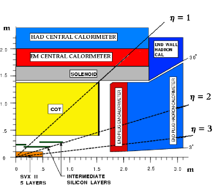
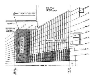
The COT detector Affolder et al. (2004) is a 96 layer, 3.2 m long open-cell drift chamber which, combined with the solenoid, is used to measure the momenta of charged particles with $|\eta_{det}|<1$. The detector extends from a radius of 40 cm to a radius of 137 cm. The 96 layers are divided into 8 “super-layers”, which alternate between super-layers where the wires are axial (i.e., parallel to the $z$ axis) and super-layers where the wires have a $\pm 2^{\circ}$ stereo angle, providing three-dimensional tracking. The calorimeter consists of a lead-scintillator electromagnetic (EM) compartment with shower position detection backed by an iron-scintillator hadronic compartment. The calorimeters are segmented in projective $\eta_{det}$–$\phi$ towers pointing to the nominal interaction point, at $z=0$. While the central calorimeter ($|\eta_{det}|<1.1$) is retained mostly unchanged from Run I Balka et al. (1988); Hahn et al. (1988); Yasuoka et al. (1988); Wagner et al. (1988); Devlin et al. (1988); Bertolucci et al. (1988), the plug calorimeter de Barbaro et al. (1995) with $1.1<|\eta_{det}|<3.6$ is a major component of the Run II upgrade (Fig. 2), and largely follows the design of the central detector. Since the calorimeter segmentation is coarse compared to the dimensions of an electron shower, position detectors (shower maximum detectors, CES in the central region and PES in the plug region) are placed at a depth of approximately six radiation lengths, roughly the position of the shower maximum, inside the EM calorimeters. These detectors measure the position and profile of the showers and help differentiate electrons from hadrons.

Figure 2: Cross section of upper part of plug calorimeter (top), and transverse segmentation, showing physical and trigger towers in a $30^{\circ}~{}\phi$ section (bottom). The logical segmentation for clustering purposes is the same except in the outer two rings ($\theta>30^{\circ}$), where two neighboring (in azimuth) $7.5^{\circ}$ towers are merged to match the $15^{\circ}$ segmentation of the central and wall calorimeters behind them.

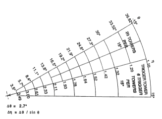
The trigger system has undergone a complete redesign as a result of the accelerator and detector upgrades. The CDF trigger is a three-level system that selects events out of a 2.5 MHz crossing rate to be written to magnetic tape at a rate of $\sim$75 Hz. The first two levels Winer (2001) are composed of custom electronics with data paths separate from the data acquisition system. The third level Anikeev et al. (2001) receives the complete detector information from the data acquisition system and runs a version of the reconstruction software optimized for speed on a farm of commercial computers. The $Z/\gamma^{*}$ events used in this measurement are selected by high-$E_{T}$ central electron triggers. At Level 1, electrons are selected by the presence of an energy deposition of $E_{T}>8$ GeV in an EM calorimeter tower and a matching two-dimensional ($r$–$\phi$ plane) track with $p_{T}>8$ GeV/$c$ reconstructed in the COT by the eXtremely Fast Tracker (XFT) Thomson et al. (2002). At Level 2, the electron energy is reconstructed in a cluster of EM towers and is required to have $E_{T}>16$ GeV. At Level 3, a reconstructed EM cluster with $E_{T}>18$ GeV and a matching three-dimensional track with $p_{T}>9$ GeV/$c$ are required. At each level, the energy in the hadronic towers just behind the EM tower or cluster is required to be less than 12.5% of the EM energy. Another trigger path that does not require a hadronic energy fraction is added to this measurement in order to improve the trigger efficiency for central electrons with very high $E_{T}$. The integrated luminosity of the data sample for this analysis is ($72\pm 4$) pb^-1.

II.2 Data samples

Four data samples are employed in this analysis. These are described briefly below and in more detail in subsequent sections.

• $Z/\gamma^{*}\rightarrow e^{+}e^{-}$ sample: A sample of 5,200 dielectron candidates is used to measure $A_{FB}$, calibrate the energy scale and resolution of the EM calorimeter, and study the material in the tracking volume.

• $W\rightarrow e\nu$ sample: A sample of 38,000 $W\rightarrow e\nu$ candidates, where the electron is reconstructed in the central calorimeter, is used to study the material in the tracking volume, to calibrate the relative calorimeter response within a central tower, and to check charge biases in measuring electrons.

• Inclusive electron sample: A sample of 3 million central electron candidates with $E_{T}>8$ GeV is used to calibrate the relative response of the central EM calorimeter towers.

• Dijet samples: A sample of 1 million dijet events (events with at least two jets, each with $E_{T}>20$ GeV) is used to measure the rate at which jets fake an electron signature and to estimate the dijet background. A jet is defined as a cluster of energy reconstructed in the calorimeter. Triggers for the sample require a calorimeter tower with $E_{T}>5$ GeV at Level 1, a calorimeter cluster with $E_{T}>15$ GeV at Level 2, and a reconstructed jet with $E_{T}>20$ GeV at Level 3. Due to the high cross section, only 1 in roughly 400 events on average were randomly selected to be recorded for this trigger. Jet samples with higher trigger thresholds (50 GeV, 70 GeV, and 100 GeV at Level 3) are also used to cross-check the fake rate for a trigger bias.

II.3 Monte Carlo samples

Monte Carlo generation and detector simulation are used to measure the acceptance for the Drell-Yan process, model the effect of radiation and detector resolution, determine the characteristics and amount of background in the data sample, and understand systematic uncertainties on the $A_{FB}$ measurement. PYTHIA Sjostrand et al. (2001) and HERWIG Corcella et al. (2001) generators with CTEQ5L PDFs Lai et al. (2000) are used for most of the samples. These generate processes at leading order and incorporate initial- and final-state QCD and QED radiation via their parton shower algorithms (HERWIG does not include final-state QED radiation). PYTHIA is tuned so that the underlying event (the remaining $\overline{p}p$ fragments from the collision) and the $p_{{}_{T}}$ spectrum of $Z$ bosons agree with the CDF data Affolder et al. (2000). Two matrix element generators, WGAMMA Baur and Berger (1990) and ALPGEN Mangano et al. (2003), are used to check the $W+X\rightarrow e\nu+X$ background estimate from PYTHIA, where $X$ is a photon or hadronic jet. The generator WGAMMA calculates the cross section of the $\mbox{$\overline{p}p$}\rightarrow W\gamma$ process. It uses electroweak helicity amplitudes for $W\gamma$ production and radiative $W$ boson decays, including all interference terms. ALPGEN performs the calculation of the matrix element for the production of $W$+quark and $W$+gluon final states. The detector simulation models the decay of generated particles and their interactions with the various elements of the CDF detector. A full GEANT3 Agostinelli et al. (2003) simulation is used to simulate the tracking volume. A parameterized simulation is used for the calorimeters and muon chambers. Comparisons between the data and Monte Carlo simulation are discussed in Sec. III.4.

There are nine Monte Carlo samples used in this analysis, which are briefly described below.

• $Z/\gamma^{*}\rightarrow\ e^{+}e^{-}$ sample: A sample generated with PYTHIA is used to calculate corrections due to acceptance, bremsstrahlung, and energy resolution, and to estimate the systematic uncertainties due to the energy scale and resolution. A quarter of the sample was generated with $M_{Z/\gamma*}>105$ GeV/$c^{2}$ to reduce the statistical uncertainties associated with the Monte Carlo sample in the high-mass region.

• $Z/\gamma^{*}\rightarrow\ e^{+}e^{-}$ sample for material systematics: Three PYTHIA samples are used to estimate the change in the measured $A_{FB}$ between the default simulation and a modified simulation which adds or subtracts $1.5\%$ radiation length ($X_{0}$) of copper in a cylinder in the central region and ${1\over 6}X_{0}$ of iron on the face of the plug calorimeter. QCD fragmentation is turned off for these samples in order to save CPU time.

• $Z/\gamma^{*}\rightarrow\ \tau^{+}\tau^{-}$ sample: A PYTHIA sample is used to estimate the background due to $Z/\gamma^{*}\rightarrow\ \tau^{+}\tau^{-}$. TAUOLA Was (2001) is used to decay $\tau$’s.

• Dijet sample: A PYTHIA sample with all $2\rightarrow 2$ processes is used to understand the characteristics of the dijet background. A lower limit of $p_{{}_{T}}>18$ GeV on the transverse momentum in the rest frame of the hard interaction is applied.

• $t\overline{t}$ sample: A HERWIG sample is used to estimate the background due to $t\overline{t}$ production.

• Diboson samples: A sample with $WW$ production and a sample with $WZ$ production are generated using PYTHIA and used to estimate the diboson backgrounds.

• $W\rightarrow\ e\nu$ sample: A PYTHIA sample is used to estimate the background due to the inclusive $W$ production.

• $W\gamma\rightarrow\ e\nu\gamma$ sample: A WGAMMA sample is used to cross-check the background due to $W+\gamma$ production.

• $W+q/g\rightarrow e\nu+q/g$ sample: An ALPGEN sample is used to estimate the background due to $W$ + quark or gluon production.

II.4 Strategy of analysis

This analysis focuses on $e^{+}e^{-}$ pair production via an intermediate $Z/\gamma^{*}$. The goal of this analysis is to measure $A_{FB}$ as a function of the invariant mass of the dielectron pair. The dielectron sample is chosen because of the low backgrounds and the good polar angle coverage of electrons in the CDF II detector.

When the incoming quarks participating in the Drell-Yan process have no transverse momentum relative to their parent baryons, $\theta$ in Eq. (6) is determined unambiguously from the four-momenta of the electrons by calculating the angle that the electron makes with the proton beam in the center-of-mass frame of the electron-positron pair. When either of the incoming quarks has significant transverse momentum, however, there exists an ambiguity in the four-momenta of the incoming quarks in the frame of the electron-positron pair, since one cannot determine the four-momenta of the quark and anti-quark individually (see Fig. 3). The Collins-Soper formalism Collins and Soper (1977) is adopted to minimize the effects of the transverse momentum of the incoming quarks in Eq. (6). (The magnitude of the effect in the Collins-Soper frame is discussed in Sec. VII.2.) In this formalism, the polar axis is defined as the bisector of the proton beam momentum and the negative of the anti-proton beam momentum when they are boosted into the center-of-mass frame of the electron-positron pair. The variable $\theta^{*}$ is defined as the angle between the electron and the polar axis. Let $Q$ ($Q_{T}$) be the four-momentum (transverse momentum) of the electron-positron pair, $P_{1}$ be the four-momentum of the electron, and $P_{2}$ be the four-momentum of the positron, all measured in the lab frame. Then $\cos\theta^{*}$ is given by

$$\mbox{$\cos\theta^{*}$}={2\over\sqrt{Q^{2}(Q^{2}+Q_{T}^{2})}}~{}(P_{1}^{+}P_{2}^{-}-P_{1}^{-}P_{2}^{+}),$$ (8)

where $P_{i}^{\pm}={1\over\sqrt{2}}(P_{i}^{0}\pm P_{i}^{3})$, and $P^{0}$ and $P^{3}$ represent the energy and the longitudinal component of the momentum, respectively. Forward events are defined as having $\mbox{$\cos\theta^{*}$}>0$ and backward events are defined as having $\mbox{$\cos\theta^{*}$}<0$.

Figure 3: Diagram of $\mbox{$\overline{p}p$}\rightarrow\mbox{$Z/\gamma^{*}$}$, where one of the quarks radiates a gluon or photon imparting transverse momentum to the quark. Once the quarks annihilate to $Z/\gamma^{*}$, the source of the transverse momentum is ambiguous.

The $A_{FB}$ measurement is made in 15 bins of $M_{ee}$ between 40 GeV/$c^{2}$ and 600 GeV/$c^{2}$. The bin sizes are chosen based on the detector $M_{ee}$ resolution and the relative Drell-Yan cross sections in each bin. Once the event selection has been made, the estimated number of forward and backward background events are subtracted from the candidate sample in each $M_{ee}$ bin. The raw forward-backward asymmetry ($A_{FB}^{raw}$) is calculated by applying Eq. (7) to the background subtracted sample.

The goal is to connect what we measure in the detector after background subtraction ($A_{FB}^{raw}$) to theoretical calculations ($A_{FB}^{phys}$). If the detector simulation is available, a direct comparison can be made between the uncorrected data and a model prediction. These comparisons are made in Sec. VII.1. If the simulation is not available, the true $A_{FB}^{phys}$ must be unfolded from $A_{FB}^{raw}$. $A_{FB}^{raw}$ must be corrected for detector acceptances and efficiencies (which sculpt the $\cos\theta^{*}$ distribution) and for smearing effects (which move events between $M_{ee}$ bins) to obtain $A_{FB}^{phys}$, which can be compared directly to theoretical calculations. The $M_{ee}$ bin migration near the $Z$ pole is not negligible, which makes it difficult to unfold $A_{FB}^{phys}$ in those bins. Performing an unconstrained unfolding analysis in those bins results in large uncertainties, while applying Standard Model or other constraints can bias the result. Two different unfolding analyses are performed to reconstruct $A_{FB}^{phys}$ with different constraints. Both unfolding analyses assume the Standard Model $\frac{d\sigma}{dM_{ee}}$ to be able to calculate the event migration effects. The uncertainties associated with systematic effects are estimated by varying the magnitude of these effects in the Monte Carlo simulation and recalculating the results for each analysis.

The first and least constrained analysis is performed by fitting for $A_{FB}^{phys}$ with a smoothing constraint. The acceptance and event migration are parameterized (Sec. V.4) to transform $A_{FB}^{phys}$ into $A_{FB}^{raw}$,

$$(\mbox{$A_{FB}^{raw}$})_{i} = g({\textbf{A}},i),$$ (9)

$$\mathrm{where}~{}{\textbf{A}} = \{(\mbox{$A_{FB}^{phys}$})_{1},(\mbox{$A_{FB}^{phys}$})_{2},\ldots,(\mbox{$A_{FB}^{phys}$})_{15}\}.$$ (10)

The probability, for a given $A_{FB}$, to find a number of forward and backward events is the binomial probability ($P[\mbox{$A_{FB}$},N^{F},N^{B}]$). The maximum likelihood method is used to obtain the 15 values of $A_{FB}^{phys}$ or A (Sec. VII.3), where the negative log likelihood with a smoothing constraint for bins near the $Z$ pole is defined as

$$\alpha={\sum_{i=1}^{15}-log(P[g({\textbf{A}},i),N^{F}_{i},N^{B}_{i}])}+{\lambda\cdot\sum_{i=2}^{9}S[{\textbf{A}}_{i}]},$$ (11)

$$\mathrm{where}~{}{\textbf{A}}_{i}=\{(\mbox{$A_{FB}^{phys}$})_{i-1},(\mbox{$A_{FB}^{phys}$})_{i},(\mbox{$A_{FB}^{phys}$})_{i+1}\},$$ (12)

$S[{\textbf{A}}_{i}]$ is a regularization function, and $\lambda$ is the regularization parameter. This analysis makes no assumptions about the shape of $A_{FB}$ (aside from it being smooth near the $Z$ pole), but it has the largest uncertainties.

In a second analysis, the parameterized acceptance and event migration are also used for the measurement of the $Z$-quark and $Z$-electron coupling constants, and $\sin^{2}\theta_{W}^{eff}$. We vary the couplings at generator level and perform a $\chi^{2}$ fit between the smeared theoretical calculations and $A_{FB}^{raw}$ to extract the couplings. This analysis is described in detail in Sec. VII.4.

Continuing with the second analysis, $A_{FB}$ can be measured by assuming the Standard Model $A_{FB}$ shape with the measured $Z$-quark couplings. In this method, acceptance correction factors ($a_{cor}^{\pm}$) are used to correct the number of forward and backward events in each $M_{ee}$ bin. The correction factor accounts for the effects of detector acceptance and efficiency, and bin migration (Sec. V.5). These correction factors depend on the input $A_{FB}^{phys}$ that is used to calculate them. To constrain the Standard Model bias, the input $A_{FB}^{phys}$ is constrained to the prediction with uncertainties from the $Z$-quark coupling analysis. Then $A_{FB}^{phys}$ can be calculated directly using the correction factors (Sec. VII.5). Equation (7) can be rewritten:

$$A_{FB}^{i} = {\left(\frac{d\sigma}{dM}\right)^{+}_{i}-\left(\frac{d\sigma}{dM}\right)^{-}_{i}\over\left(\frac{d\sigma}{dM}\right)^{+}_{i}+\left(\frac{d\sigma}{dM}\right)^{-}_{i}},$$ (13)

where

$$\left(\frac{d\sigma}{dM}\right)^{\pm}_{i} = {\frac{(N^{\pm}_{i}-B^{\pm}_{i})}{\Delta M_{i}L(a_{cor}^{\pm})_{i}}}.$$ (14)

In Eq. (14), $\Delta M_{i}$ is the size of the i-th mass bin, and $L$ is the integrated luminosity. $N^{+}(N^{-})$ and $B^{+}(B^{-})$ are the number of candidate and estimated background events in the forward (backward) region, respectively. Canceling common factors, the forward-backward asymmetry can be written as

$$A_{FB}^{i} = {\frac{\frac{N^{+}_{i}-B^{+}_{i}}{(a_{cor}^{+})_{i}}-\frac{N^{-}_{i}-B^{-}_{i}}{(a_{cor}^{-})_{i}}}{\frac{N^{+}_{i}-B^{+}_{i}}{(a_{cor}^{+})_{i}}+\frac{N^{-}_{i}-B^{-}_{i}}{(a_{cor}^{-})_{i}}}}.$$ (15)

The analysis using correction factors has smaller uncertainties than the unconstrained method, but it assumes no non-standard physics outside of deviations in $Z$-quark couplings. This analysis technique is similar to the Run I measurement.

While these analyses make different constraints on the form of $A_{FB}$, it is important to note that they should give similar results in bins where there is a negligible amount of event migration between $M_{ee}$ bins. At high mass, where the bin sizes are very large compared to the detector resolution, the results are independent of the unfolding method.

III Electron measurement

This analysis requires two electrons ($e^{+},e^{-}$) in the event, one in the central region, and the other in the central or plug region. This section describes the identification of central and plug electrons, the event selection criteria, the electron energy scale and resolution, and the charge identification of electrons. In most cases, discussion of electrons refer to both electrons and positrons.

III.1 Central electron identification

Electron identification in the central calorimeter is almost identical to the algorithm used in Run I, since the calorimeter is unchanged and the new drift chamber has a geometry very similar to the previous one. For a more detailed description of the central electron reconstruction variables see Ref. Abe et al. (1994). An electron candidate is reconstructed if there is a central tower with $E_{T}>2$ GeV and a charged drift chamber track that extrapolates to the tower. The adjacent towers on either side in $\eta_{det}$ are added to the cluster, and the cluster is not accepted if the energy in the hadronic part is more than 12.5% of the energy in the EM part. An electron is considered within the fiducial region of the detector if its track points within 60 cm in $z$ of the center of the detector and extrapolates to the calorimeter away from any wedge boundaries. (A wedge consists of those towers with the same value of $\phi$.) The polar range of electrons in the central region is $|\eta_{det}|<1.0$. The energy of the electron is determined by the total energy it deposits in the EM calorimeter. The momentum ($p_{{}_{T}}$) of the electron is determined by the highest-$p_{{}_{T}}$ COT track associated with the EM cluster. The track is constrained to the position of the beamline in $r$–$\phi$. The direction of the electron’s momentum is taken from the direction of the track and is used in the calculations of the transverse component of the energy ($E_{T}$) and the invariant mass of the electron pairs. The charge of the electron ($q$) is determined from the curvature of the track. The variables that are used to discriminate electrons from hadrons are: (1) the ratio of the hadronic energy to the electromagnetic energy ($E_{had}/E_{em}$); (2) the total transverse energy within a radius of 0.4 in $\Delta R=\sqrt{\Delta\eta_{evt}^{2}+\Delta\phi^{2}}$ of the cluster centroid, excluding the cluster energy itself ($E_{T}^{iso}$);(3) the ratio of the calorimeter energy to the momentum of the track ($E/p$); (4) the comparison of the lateral sharing of energy among the calorimeter towers with that of test beam electron data ($L_{shr}$); (6) a $\chi^{2}$ comparison of the shower profile measured by the shower maximum detector with the shower profile measured from test beam electrons ($\chi^{2}_{strip}$); (5) the distance in $r$–$\phi$ and $z$ between the electron shower position measured by the shower maximum detector and the extrapolated track position ($q\cdot\Delta x$ and $\Delta z$). An asymmetric cut is made on $q\cdot\Delta x$ because bremsstrahlung distorts the shower shape in the $r$–$\phi$ direction. Since the magnetic field bends an electron’s trajectory, but not a photon’s, the bremsstrahlung photons tend to enter the calorimeter to the side of the primary electron opposite the bending, which is determined by the electron’s charge. By multiplying the charge by $\Delta x$, most of the distortion from bremsstrahlung photons is isolated to $q\cdot\Delta x<0$.

III.2 Plug electron identification

The electron clusters in the plug region, subtending $1.2<|\eta_{det}|<3.0$, are limited to $2\times 2$ towers (two towers in pseudorapidity by two towers in azimuth). Since the Moliere radius of a typical electron shower is significantly smaller than the size of the plug EM towers, the clusters fully contain electron energies. As with the central clusters, plug electron clusters are accepted if $E_{had}/E_{em}<12.5\%$. The major difference between central and plug electrons is the tracking. In the central region, the COT tracking is very efficient ($99.6\%$), whereas in the plug region the efficiency rapidly falls off as $|\eta_{det}|$ increases due to the geometrical acceptance of the COT. In this analysis no tracking is used for plug electrons. The $z$ position of the collision for the event ($z_{vertex}$) is provided by the $z$ position of the central electron’s track. The electron’s shower centroid is determined from a fit of the energy distribution among the calorimeter towers. The direction of the plug electron is determined by extrapolating from $z_{vertex}$ to the shower centroid. The unmeasured charge of the plug electron is assumed to be the opposite of the central electron. The following variables are used to discriminate electrons from hadrons in the plug region : (1) the ratio of the hadronic energy to the EM energy ($E_{had}/E_{em}$); (2) the total transverse energy within a radius of 0.4 in $\Delta R=\sqrt{\Delta\eta_{evt}^{2}+\Delta\phi^{2}}$ of the cluster centroid, excluding the cluster energy itself ($E_{T}^{iso}$); (3) a $\chi^{2}$ comparison of the energy distribution in $3\times 3$ EM towers around the seed tower to the energy distributions from test beam electrons ($PEM\chi_{3\times 3}^{2}$). The selection criteria for plug electrons are summarized in Table 1.

III.3 Event selection

$Z/\gamma^{*}\rightarrow\ e^{+}e^{-}$ candidate events are required to have two electrons with $E_{T}>20$ GeV. One of the electrons is required to be in the central region and to pass the full set of identification cuts (see Table 1). This electron is called the central-tight electron. The second loose electron is allowed to be in either the central or plug region and has relaxed identification cuts for higher efficiency (see Table 1). Based on these selection criteria, two topologies are defined for dielectron events: central-central topology, where one central-tight and one central-loose electron are required, and central-plug topology, where one central-tight electron and one plug-loose electron are required. In the central-central topology, the two electrons are required to have opposite charge. In the central-plug topology, no charge requirement is made since the plug electron’s charge is not measured.

Variable	Central-Tight	Central-Loose	Plug-Loose
$E_{T}$	$>20$ GeV	$>20$ GeV	$>20$ GeV
$p_{T}$	$>10$ GeV	$>10$ GeV	N/A
$E_{had}/E_{em}$	$<0.055$	$<0.055$	$<0.05$
	$~{}~{}+0.00045*E$	$~{}~{}+0.00045*E$
$E_{T}^{iso}$	$<4$ GeV	$<4$ GeV	$<4$ GeV
$E/p$	$<2$	no cut	N/A
	for $E_{T}<50$ GeV
$L_{shr}$	$<0.2$	no cut	N/A
$\chi_{strip}^{2}$	$<10$	no cut	N/A
$q*\Delta x$	$>-3$ cm,	no cut	N/A
	$<1.5$ cm
$|\Delta z|$	$<3$ cm	no cut	N/A
$PEM\chi_{3\times 3}^{2}$	N/A	N/A	$<10$

Table 1: Criteria for electron candidates. $Z/\gamma^{*}\rightarrow\ e^{+}e^{-}$ candidates require at least one central-tight electron and at least one additional loose electron (central or plug) in the event.

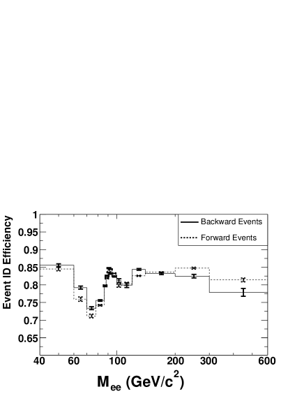
The absolute identification efficiencies are measured from the $Z/\gamma^{*}\rightarrow\ e^{+}e^{-}$ data where one electron is selected using the central-tight electron cuts, and the second electron is used as a probe to measure the identification efficiencies. The total identification efficiencies are found to be $(83.4\pm 0.8)\%$ for central-tight electrons, $(94.3\pm 0.5)\%$ for central-loose electrons, and $(87\pm 2)\%$ for plug-loose electrons. Since we measure the ratios of forward and backward events to the total events, only the relative difference in efficiencies between forward and backward events affects the $A_{FB}$ measurement. The relative efficiencies and their dependence on $M_{ee}$ are estimated from the Monte Carlo simulation (see Fig. 4). The difference between the forward and backward event efficiencies is largest just below the $Z$ pole. The dip in efficiency below the $Z$ pole is due to contamination from mis-measured events from the pole. The events are mis-measured due to photon radiation which also lowers the electron identification efficiency. The forward efficiency is lower because the events are more forward at the $Z$ pole, resulting in more contamination for forward events.

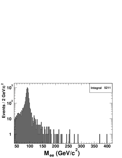
Based on these selection criteria, we find 1,892 central-central and 3,319 central-plug $Z/\gamma^{*}\rightarrow\ e^{+}e^{-}$ candidates. The invariant-mass distribution is shown in Fig. 5 and the number of events in each mass bin is given in Table 2.

Figure 4: Event electron identification efficiency, $(\epsilon_{i}^{\pm})_{ID}$, as a function of $M_{ee}$ measured from the $Z/\gamma^{*}\rightarrow\ e^{+}e^{-}$ simulation. The dashed line is for forward events and the solid line is for backward events. The dip in efficiency below 90 GeV/$c^{2}$ and the differences between forward and backward efficiencies are due to radiation effects (see Sec. III.3).

Mass Region	C-C	C-P
$40\leq\mbox{$M_{ee}$}<60$ GeV/$c^{2}$	69	85
$60\leq\mbox{$M_{ee}$}<70$ GeV/$c^{2}$	42	72
$70\leq\mbox{$M_{ee}$}<78$ GeV/$c^{2}$	48	119
$78\leq\mbox{$M_{ee}$}<86$ GeV/$c^{2}$	204	329
$86\leq\mbox{$M_{ee}$}<88$ GeV/$c^{2}$	151	299
$88\leq\mbox{$M_{ee}$}<90$ GeV/$c^{2}$	301	512
$90\leq\mbox{$M_{ee}$}<92$ GeV/$c^{2}$	416	610
$92\leq\mbox{$M_{ee}$}<94$ GeV/$c^{2}$	330	543
$94\leq\mbox{$M_{ee}$}<100$ GeV/$c^{2}$	243	545
$100\leq\mbox{$M_{ee}$}<105$ GeV/$c^{2}$	30	68
$105\leq\mbox{$M_{ee}$}<120$ GeV/$c^{2}$	29	61
$120\leq\mbox{$M_{ee}$}<140$ GeV/$c^{2}$	13	31
$140\leq\mbox{$M_{ee}$}<200$ GeV/$c^{2}$	9	36
$200\leq\mbox{$M_{ee}$}<300$ GeV/$c^{2}$	6	8
$300\leq\mbox{$M_{ee}$}<600$ GeV/$c^{2}$	1	1

Table 2: The number of central-central (C-C) and central-plug (C-P) $Z/\gamma^{*}\rightarrow\ e^{+}e^{-}$ candidates in each mass region.

Figure 5: Distribution of dielectron invariant mass from $Z/\gamma^{*}\rightarrow\ e^{+}e^{-}$ candidates in 72 pb^-1 of Run II data.

III.4 Detector simulation of $Z/\gamma^{*}\rightarrow\ e^{+}e^{-}$

The simulation is used to understand the detector’s geometric acceptance for electrons, bremsstrahlung radiation from interactions with the detector material, and the energy scale and resolution for electrons in the tracking chambers and calorimeters. In this section, comparisons of the kinematic and geometric distributions between the data and simulation are discussed, and any discrepancies are presented as a possible systematic uncertainty.

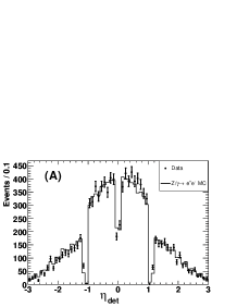
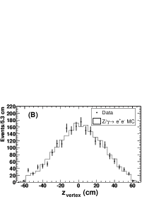
The geometric acceptance is largely dependent on the location of the $\overline{p}p$ interaction vertex ($z_{vertex}$ distribution) and the geometric description of the detector. Figure 6A shows the distribution of $\eta_{det}$ for electrons in the $Z/\gamma^{*}\rightarrow\ e^{+}e^{-}$ data sample compared with the prediction from the Monte Carlo simulation. The discrepancies shown in Fig. 6A are used to estimate a systematic uncertainty on the fiducial acceptance (see Sec. VI). The Monte Carlo simulation correctly models the observed $z_{vertex}$ distribution (Fig. 6B). Fitting the $z_{vertex}$ distribution to a Gaussian function yields an average position in $z$ of $+2.5$ cm and a width of 28 cm.

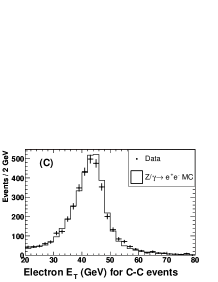
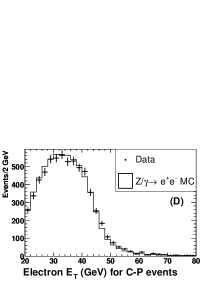
The calorimeter energy scale and resolution in the simulation are tuned so that the mean and width of the $Z\rightarrow e^{+}e^{-}$ peak in the simulation are consistent with those from the data (see Sec. III.5). The $E_{T}$ distribution of the electrons for central-central and central-plug events after the simulation tuning are shown in Figs. 6C and 6D. (The background prediction included in these plots is discussed in Sec. IV.)

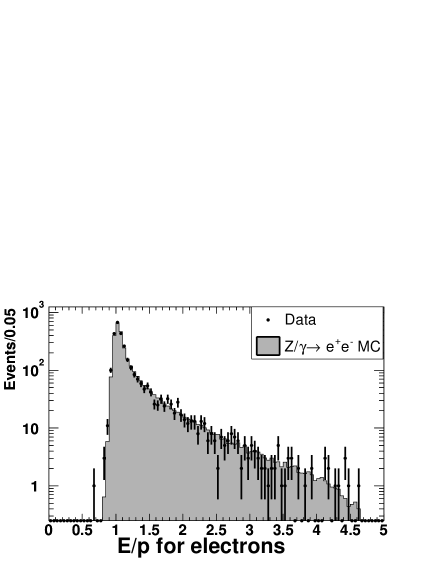
The amount of material between the collision point and the outer cylinder of the COT is tuned so that the electron identification variables sensitive to external bremsstrahlung in the data match with those in the simulation (see Sec. III.6). The material in the Monte Carlo simulation between the interaction point and the tracking volume is tuned using the $E/p$ distribution as shown in Fig. 7. The ratio between the number of events in the high tail ($E/p>2$) and that in the peak is used to calibrate and determine an uncertainty due to the modeling of the material in the detector simulation.

Figure 6: The electron $\eta_{det}$(A) and event vertex $z$ position (B) are important for understanding the geometric acceptance in the simulation. The electron $E_{T}$ distribution for central-central(C), and central-plug(D) are used to the kinematic distributions. The Monte Carlo histograms are normalized to the number of entries in the background-subtracted data. The detector simulation for electrons has been tuned so that the $Z$ peak and width match the data (Sec. III.5). The discrepancies are used to estimate systematic uncertainties on the Monte Carlo simulation (see Sec. VI).

Figure 7: The $E/p$ distribution for central electrons in the $Z/\gamma^{*}\rightarrow\ e^{+}e^{-}$ data sample. Points and histograms are data and Monte Carlo simulation, respectively. The Monte Carlo histogram is normalized to the number of entries in the data. The high tail ($E/p>2$) of this distribution is used to calibrate the amount of material in the Monte Carlo simulation between the interaction point and the tracking volume.

III.5 Electron energy scale and resolution

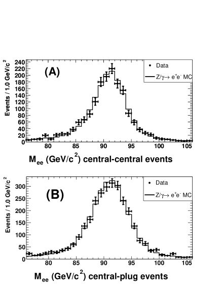
Both local and global energy scale corrections are applied to the electron energy. Local corrections are applied to improve resolution by correcting for variations in the energy response of the calorimeter. They include corrections for time dependence, variations in the response at different points within a calorimeter tower Yasuoka et al. (1988), and variations in the gains of the different calorimeter tower channels. Electrons from the $W$ sample and the inclusive electron sample are used to calibrate these variations. The reference for correcting the electron energy is the track momentum as measured by the COT. Uniformity is achieved by adjusting the tower energy responses (gains) until the mean $E/p$ is flat as a function of time and $\phi$, and agrees with the Monte Carlo simulation as a function of $\eta$. Figure 8 shows the invariant-mass distributions near the $Z$ peak for central-central and central-plug events for data and Monte Carlo simulation. High-energy electrons are measured with a resolution of $\frac{\sigma(E_{T})}{E_{T}}=\frac{13.5\%}{\sqrt{E_{T}}}\oplus 1.5\%$ Balka et al. (1988) in the central calorimeters and $\frac{\sigma(E)}{E}=\frac{14.4\%}{\sqrt{E}}\oplus 0.7\%$ Albrow et al. (2002) in the plug calorimeters.

Figure 8: Invariant-mass distributions of $Z/\gamma^{*}\rightarrow\ e^{+}e^{-}$ candidates: two electrons in the central region (top), one electron in the central region and the other in the plug region (bottom). Points and histograms are data and Monte Carlo simulation, respectively. Energy scale corrections and extra energy smearing are applied to the simulation so that the Gaussian widths and peaks match.

III.6 Electron charge identification

The charge measurement of electrons is essential for this analysis because the charge determines the sign of $\cos\theta^{*}$ (see Eq. (8)), and therefore determines whether the event is forward or backward. In the central-central topology, we measure the charge of both electrons and require that they have opposite sign. The central-central opposite-sign requirement removes events where one of the electrons has a misidentified charge from the event sample, leaving very little ambiguity on the forward-backward measurement due to charge misidentification. However, in events with a central-plug topology, the charge of the two electrons is determined solely from the central electron. So a misidentification of the central electron’s charge will switch the sign on $\cos\theta^{*}$, and result in a misassignment of the event as forward or backward. For this reason, the charge misidentification rate needs to be properly understood, and well modeled by the simulation.

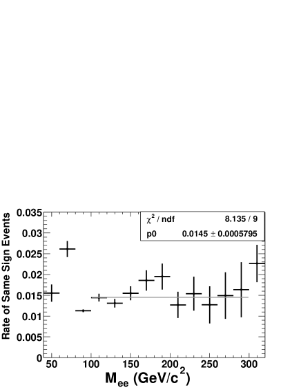
We use the $Z/\gamma^{*}\rightarrow\ e^{+}e^{-}$ Monte Carlo sample with the central-central topology to study the sources of charge misidentification and to measure the misidentification rate. The misidentification rate is determined by counting the number of events where both electrons have the same charge. If the rate is small, the probability of having same-sign events is approximately twice that of misidentifying the charge of a single electron. Figure 9 shows that above the $Z$ pole ($\mbox{$M_{ee}$}>100$ GeV/$c^{2}$), the rate of events with the same sign is approximately flat up to $\mbox{$M_{ee}$}\simeq 300$ GeV/$c^{2}$. The drop in the rate at the $Z$ pole and the increase in the rate in the next lower bin are attributable to hard bremsstrahlung followed by $e^{+}e^{-}$ pair production in the material. This process is referred to as charge misidentification due to “trident” electrons. Figure 10 shows a “trident” electron where a positron radiates a hard bremsstrahlung photon in the material, and the photon subsequently converts into an electron-positron pair in the material. The electron from the photon conversion carries the highest momentum, and the charge of the primary electron ($e^{+}$) is assigned to be negative $(e^{-})$. The Monte Carlo sample shows that the charge misidentification rate coming from “trident” electrons is $(0.7\pm 0.3)\%$. The other source of charge misidentification is the drift chamber tracking resolution of $\delta({\frac{1}{p_{{}_{T}}}})\simeq 0.001$ GeV^-1. At higher energies, the tracks become almost straight ($\frac{1}{p_{{}_{T}}}\sim 0$), and the charge determination has a higher probability of being wrong. The last bin, which includes all events with $\mbox{$M_{ee}$}>300$ GeV/$c^{2}$, has a misidentification rate measured from the simulation of $(1.1\pm 0.2)\%$. Corrections for charge misidentification are included as part of the acceptance calculation via simulation. The dominant systematic uncertainty comes from the uncertainty in the amount of material between the interaction point and the tracking volume. A comparison of the same-sign events between data and Monte Carlo simulation is used to get an estimate on the background. The comparison shows agreement at the $Z$ pole where there is little background (Fig. 15).

Figure 9: The rate of same-sign events as a function of the dielectron invariant mass from the $Z/\gamma^{*}\rightarrow\ e^{+}e^{-}$ Monte Carlo sample. The rate of charge misidentification is half of the same-sign event rate. The last bin shows the rate for all events with $\mbox{$M_{ee}$}>300$ GeV/$c^{2}$. A fit to a constant between 100 GeV/$c^{2}<\mbox{$M_{ee}$}<300$ GeV/$c^{2}$ has been made with the result that $Z/\gamma^{*}$events have an average same-sign rate (p0) of 1.45%.

Figure 10: A schematic diagram of a “trident” electron where a positron radiates a hard bremsstrahlung photon in the material and the photon converts into an electron-positron pair in the material. The electron from the photon conversion carries the highest momentum, thus the charge of the primary electron ($e^{+}$) is assigned to be negative $(e^{-})$.

III.7 Charge dependence of electron efficiencies

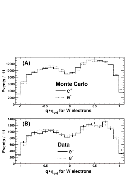
A systematic bias in the forward-backward asymmetry may occur if the detector response to electrons differs from that to positrons. We compare acceptances and efficiencies for electrons and positrons using the $W^{\pm}\rightarrow e^{\pm}\nu$ Monte Carlo and data samples. In Fig. 11, the number of $e^{+}$ events and $e^{-}$ events are plotted as a function of $q\cdot\eta_{det}$ of the electrons. The difference between the $q\cdot\eta_{det}<0$ region and the $q\cdot\eta_{det}>0$ region comes from the intrinsic charge asymmetry in $W^{\pm}$ production in the proton direction and the anti-proton direction. Because the average momentum of $u$ ($\bar{u}$) quarks is larger than that of $d$ ($\bar{d}$) quarks in the proton (anti-proton), $W^{+}$ ($W^{-}$) event production is enhanced in the proton (anti-proton) direction.

Small differences are observed in the data between the $e^{+}$ and $e^{-}$ yields (Fig. 11B). These could be caused by differences in the detector response between electrons and positrons, differences between the $|\eta_{det}|>0$ and $|\eta_{det}|<0$ detectors, or an asymmetric $z_{vertex}$ distribution about 0. Similar differences are seen in the Monte Carlo sample (Fig. 11A) where the differences come purely from the asymmetric $z_{vertex}$ distribution (see Sec. II.3). The asymmetry between the $e^{+}$ and $e^{-}$ yields due to the asymmetric $z_{vertex}$ distribution is measured to be $(0.7\pm 0.2)$% from the simulation. After the effect of the $z_{vertex}$ offset is taken into account, the observed asymmetry in the data is reduced to $(0.1\pm 0.7)$%. The impact of this asymmetry on the forward-backward charge asymmetry measurement is therefore estimated to be small compared to other sources of systematic uncertainties.

Figure 11: The $q\cdot\eta_{evt}$ distribution of the electrons in $W$ Monte Carlo (A) and data (B) events. The asymmetry about 0 is due to the charge asymmetry in the $W$ production. The difference between $e^{+}$ and $e^{-}$ is largely due to the asymmetric distribution of the event vertex ($z_{vertex}$) distribution.

IV Backgrounds

The dominant sources of background to the process $\mbox{$\overline{p}p$}\rightarrow\mbox{$Z/\gamma^{*}\rightarrow\ e^{+}e^{-}$}+X$ are:

1. Dijet events where the jets are misidentified as electrons,

2. $W+X\rightarrow e\nu+X$, where $X$ is a photon or a jet misidentified as an electron,

3. $\mbox{$Z/\gamma^{*}\rightarrow\ \tau^{+}\tau^{-}$}\rightarrow\mbox{$e^{+}e^{-}$}\nu_{\tau}\nu_{e}\bar{\nu}_{\tau}\bar{\nu}_{e}$,

4. $\mbox{$W^{+}W^{-}$}\rightarrow\mbox{$e^{+}e^{-}$}\nu_{e}\bar{\nu}_{e}$,

5. $W^{\pm}Z$ where $Z\rightarrow\ e^{+}e^{-}$,

6. $\mbox{$t\overline{t}$}\rightarrow\mbox{$e^{+}e^{-}$}\nu_{e}\bar{\nu}_{e}\mbox{$b\overline{b}$}$.

The determination of $A_{FB}$ requires knowledge of the number of background events and the forward-backward charge asymmetry of the background events in each mass bin.

IV.1 Dijet background

Dijet events are the dominant source of background in our sample. This background category includes events with two high-$p_{{}_{T}}$ jets and those with one jet and one photon. Hadrons in jets can be misidentified as electrons, and jets can contain real electrons produced in semi-leptonic heavy-flavor decays (from $c$ or $b$ quarks). Photons from initial- or final-state bremsstrahlung are identified as electrons if they are in the plug region. In the central region, photons must convert in order to be identified as electrons because of the tracking requirement. The physics objects producing electron candidates in dijet events are discussed in Sec. IV.1.1. The forward-backward charge asymmetry from the dijet background is discussed in Sec. IV.1.2. In Sec. IV.1.3, the rate of jets faking electrons is measured, the dijet background in the data is estimated, and the invariant-mass distribution of the dijet background is extracted. In Sec. IV.1.4, the amount of dijet background in the central-central topology is cross-checked using same-sign events in the $Z/\gamma^{*}$ data and Monte Carlo samples.

IV.1.1 Sources of electron fakes from dijet Monte Carlo

The Monte Carlo sample of $\sim$750,000 dijet events is used to understand the sources of high-$p_{{}_{T}}$ fake electrons. We find 47 central-tight electrons, 179 central-loose electrons, and 1702 plug-loose electrons in this sample. We then look for hadron jets or photons with $E_{T}>15$ GeV that match the direction of these fake electrons. The dominant sources for central-tight electrons are photons which have converted and light quark jets (those originating from $u$, $d$, and $s$ quarks). Light quark jets are the dominant source for the loose electrons, especially the plug electrons. The fraction of events found in each category is shown in Table 3.

Dijet Events

Electron Type	Light-Quark Jets	Heavy-Quark Jets	Gluon Jets	Photons
Central-Tight	0.38 $\pm$ 0.09	0.15 $\pm$ 0.06	0.13 $\pm$ 0.05	0.34 $\pm$ 0.09
Central-Loose	0.63 $\pm$ 0.06	0.08 $\pm$ 0.02	0.20 $\pm$ 0.03	0.09 $\pm$ 0.02
Plug-Loose	0.82 $\pm$ 0.02	0.01 $\pm$ 0.00	0.07 $\pm$ 0.01	0.10 $\pm$ 0.01

$W\rightarrow\ e\nu$ Events

Electron Type	Light-Quark Jets	Heavy-Quark Jets	Gluon Jets	Photons
Central-Tight	0.28 $\pm$ 0.09	0.00 $\pm$ 0.00	0.00 $\pm$ 0.00	0.72 $\pm$ 0.15
Central-Loose	0.63 $\pm$ 0.09	0.01 $\pm$ 0.01	0.01 $\pm$ 0.01	0.35 $\pm$ 0.07
Plug-Loose	0.20 $\pm$ 0.03	0.01 $\pm$ 0.01	0.01 $\pm$ 0.01	0.78 $\pm$ 0.07

Table 3: The physics objects producing electron candidates in Monte Carlo dijet and $W\rightarrow\ e\nu$ events and their fractional contributions for central-tight electrons, central-loose electrons, and plug-loose electrons. The fractional contribution of the different physics objects producing electron candidates varies depending on the type of electron and background type. Light-quark jets are those originating from $u$, $d$, and $s$ quarks, and heavy-quark jets are those originating from to $b$ and $c$ quarks. Uncertainties include only Monte Carlo statistics.

IV.1.2 Charge correlation and $A_{FB}$ distribution of dijet events

We do not expect any correlation between the charges of the two fake electrons in the dijet events. This expectation is checked using the hadron-enriched data sample, where both electrons are “jet-like”; events collected with the high-$p_{{}_{T}}$ central electron triggers that have two electromagnetic clusters passing the kinematic cuts for electrons in this analysis and a significant amount of energy near them ($E_{T}^{iso}>4$ GeV). An additional cut of $\mbox{$\not\!\!E_{t}$}~{}<~{}10$ GeV eliminates a large fraction of the remaining $W\rightarrow\ e\nu$ contamination in the sample. The selection criteria are summarized in Table 4. The sample contains 8595 (8797) events where the two electron candidates have the same (opposite) charge. Although the difference is statistically significant (2.2$\sigma$), there are only 2% more opposite-sign events than same-sign events. This demonstrates that the charges of the two electrons identified in dijet events are nearly uncorrelated.

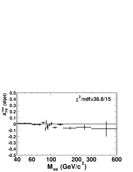
The raw forward-backward asymmetry of the dijet background is measured with the same hadron-enriched sample in the 15 mass regions. As shown in Fig. 12, the $A_{FB}^{raw}$ values are close to zero, consistent with the symmetric angular distribution expected for dijet events. This analysis assumes $\mbox{$A_{FB}^{raw}$}=0$ for the dijet background, where the events are split evenly between forward and backward categories when subtracted from the candidate sample. The measured asymmetries listed in Table 5 are used for estimating a systematic uncertainty on this assumption.

Hadron-enriched selection
$p_{{}_{T}}>10$ GeV/$c$ (central only)
$E_{T}^{corrected}>20$ GeV
$E_{T}^{iso}>4$ GeV
$\mbox{$\not\!\!E_{t}$}<10$ GeV

Table 4: Selection criteria for the hadron-enriched data sample.

Figure 12: $A_{FB}^{raw}$ of dijet background estimated from the hadron-enriched data sample.

Mass Region	# Events		$A_{FB}^{raw}$(dijet)
GeV/$c^{2}$	C-C	C-P
$40\leq M_{jj}<60$	$5.4\pm 1.9$	$51\pm 18$	0.00 $\pm$ 0.01
$60\leq M_{jj}<70$	$1.5\pm 0.5$	$25.7\pm 9.0$	0.00 $\pm$ 0.01
$70\leq M_{jj}<78$	$0.7\pm 0.2$	$15.3\pm 5.4$	-0.01 $\pm$ 0.01
$78\leq M_{jj}<86$	$0.4\pm 0.1$	$11.1\pm 3.9$	0.01 $\pm$ 0.01
$86\leq M_{jj}<88$	$0.1\pm 0.04$	$2.2\pm 0.8$	-0.09 $\pm$ 0.03
$88\leq M_{jj}<90$	$0.1\pm 0.04$	$1.9\pm 0.7$	0.00 $\pm$ 0.03
$90\leq M_{jj}<92$	$0.1\pm 0.04$	$1.8\pm 0.6$	-0.02 $\pm$ 0.03
$92\leq M_{jj}<94$	$0.1\pm 0.04$	$1.6\pm 0.6$	-0.02 $\pm$ 0.03
$94\leq M_{jj}<100$	$0.1\pm 0.04$	$4.1\pm 1.4$	-0.03 $\pm$ 0.02
$100\leq M_{jj}<105$	$0.1\pm 0.04$	$2.6\pm 0.9$	-0.02 $\pm$ 0.02
$105\leq M_{jj}<120$	$0.2\pm 0.07$	$4.8\pm 1.7$	-0.04 $\pm$ 0.01
$120\leq M_{jj}<140$	$0.1\pm 0.04$	$2.9\pm 1.0$	-0.02 $\pm$ 0.02
$140\leq M_{jj}<200$	$0.1\pm 0.04$	$1.9\pm 0.7$	-0.05 $\pm$ 0.02
$200\leq M_{jj}<300$	$0.0\pm 0.00$	$0.2\pm 0.07$	-0.01 $\pm$ 0.03
$300\leq M_{jj}<600$	$0.0\pm 0.00$	$0.0\pm 0.00$	-0.07 $\pm$ 0.11
Total	$9.0\pm 3.2$	$128\pm 45$	N/A

Table 5: The estimated number of events and measured $A_{FB}^{raw}$ of dijet background in each invariant-mass bin. The number of events is estimated using the rate of jets faking electrons. The $A_{FB}^{raw}$(dijet) values are measured from the hadron-enriched data sample. When calculating $\mbox{$A_{FB}$}(\mbox{$Z/\gamma^{*}\rightarrow\ e^{+}e^{-}$})$, $A_{FB}^{raw}$(dijet) = 0 is assumed. The measured $A_{FB}^{raw}$(dijet) is used to estimate a systematic uncertainty on the measurement.

IV.1.3 Estimation and $M_{ee}$ distribution of the dijet background

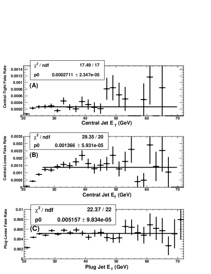
The dijet sample used to calculate the fraction of jets faking electrons (the single-jet fake rate) must pass the 20 GeV single-jet triggers, have two jets with $E_{T}>20$ GeV, have $\mbox{$\not\!\!E_{t}$}<10$ GeV, and have no more than one loose electron in the event. Jets are clustered using a cone size of $\Delta R=0.4$. These requirements ensure that the electroweak contamination from $W$ and $Z$ decays to electrons is negligible. The fake rate is defined as the fraction of jets in the sample which pass the electron-selection criteria. The measured rate is plotted as a function of jet $E_{T}$ in Fig. 13. Due to the bigger cluster size of jets compared to electrons, jet energies are larger than the corresponding fake-electron energies. For example, when a jet of $E_{T}=25$ GeV fakes an electron, the electron candidate is typically reconstructed with an $E_{T}$ of 20 GeV. The single-jet fake rate with $E_{T}^{jet}>25$ GeV (or $E_{T}^{e}>20$ GeV) is measured to be $(2.7\pm 0.2)\times 10^{-4}$ for central-tight electrons. Note that jets used in this measurement are a mixture of both triggered and non-triggered jets.

The single-jet fake rate for non-triggered jets can be measured using jets with $E_{T}$ below trigger thresholds. We use jets with $E_{T}<45$ GeV in the jet 50 GeV data sample (50 GeV single jet triggers) and $E_{T}<95$ GeV in the jet 100 GeV data sample (100 GeV single jet triggers). In addition, Monte Carlo dijet events without trigger requirements are studied for comparison. Table 6 summarizes the rates in the four different samples. The fake rate for jets without trigger biases are roughly one half of the fake rate measured in the 20 GeV dijet sample. The difference in rates is expected since the trigger requirements select jets that deposit a significant fraction of their energy into one tower and hence look more “electron-like.”

The number of dijet background events in the $Z/\gamma^{*}\rightarrow\ e^{+}e^{-}$ sample is estimated by applying the average single-jet fake rate for a tight electron and a loose electron to every pair of jets in the 20 GeV dijet sample that pass the kinematic cuts. The systematic uncertainty on this estimation is determined by taking the simplified case where each event has two and only two jets, one triggered and one non-triggered. Let $f$ denote the fake rate without trigger biases and $2f$ the average fake rate in the 20 GeV dijet sample (as described in the previous paragraph). Then, the fake rate for the triggered jets is $3f$. The event fake rate is estimated to be $4f^{2}$ if the average fake rate is applied to both jets (used for the estimation of the dijet background), and it is $3f^{2}$ if the rates for the non-triggered and triggered jets are applied separately. The difference between these two estimates, which is 25%, is taken as a systematic uncertainty on the single-jet fake rate due to the jet trigger bias.

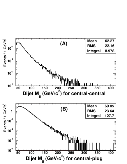
The invariant-mass distribution of the dijet background is determined from the 20 GeV dijet sample where at least one of the two jets is found in the central region. Jet energies are corrected to represent electron energies where the correction factors are determined from Gaussian fits to the $\frac{E_{T}^{e}}{E_{T}^{jet}}$ distributions for each of the three categories of electrons. (The Gaussian fits to $\frac{E_{T}^{e}}{E_{T}^{jet}}$ have means ranging from 0.88-0.92, and have widths ranging from 0.05-0.09 depending on the type of electron.) Figure 14 shows the invariant-mass distribution of the central-central and central-plug dijet events, weighted by the probability of faking a dielectron candidate event. Table 5 shows the number of dijet events expected in each invariant-mass bin. The total number of dijet background candidates is estimated to be $9.0\pm 3.2$ for the central-central topology, and $128\pm 45$ for the central-plug topology. The invariant-mass distribution of the dijet background along with the Monte Carlo $Z/\gamma^{*}\rightarrow\ e^{+}e^{-}$ prediction is shown in Fig. 21.

	Central-Tight	Central-Loose	Plug-Loose
	Rate $(\times 10^{-4})$	Rate $(\times 10^{-4})$	Rate $(\times 10^{-4})$
20 GeV dijet	$2.7\pm 0.2$	$13.7\pm 0.6$	$51.6\pm 1.0$
50 GeV dijet	$1.3\pm 0.2$	$6.5\pm 0.4$	$30.2\pm 1.2$
100 GeV dijet	$1.7\pm 0.3$	$5.5\pm 0.5$	$27.6\pm 1.8$
Monte Carlo	$1.3\pm 0.3$	$7.6\pm 0.9$	$24.8\pm 3.1$

Table 6: The rate at which a jet fakes an electron. The jets in the 20 GeV dijet sample are a mixture of triggered and non-triggered jets. The rate in the 50 GeV and 100 GeV dijet samples is measured only for jets with $E_{T}$ below the trigger threshold, $E_{T}<$ 45 (95) GeV for the 50 (100) GeV dijet sample. The rate in Monte Carlo dijet events is measured for jets with $E_{T}>$20 GeV.

Figure 13: The rate of jets faking electrons for central-tight (A), central-loose (B), and plug-loose (C) requirements in the 20 GeV dijet sample. The fake rate is measured for jets with $E_{T}^{jet}>24$ GeV for central-tight and plug-loose electrons, and $E_{T}^{jet}>26$ GeV for central-loose electrons to take into account relative energy differences between jet clustering and electron clustering. p0 is the value returned by the fit for a zeroth order polynomial.

Figure 14: The invariant-mass distribution measured in the 20 GeV dijet sample. The single-jet fake rate is applied to each jet in the dijet pair. The jet energy has been corrected to represent electron energies (see Sec. IV.1.3).

IV.1.4 Check of dijet background using the charge of the dielectrons

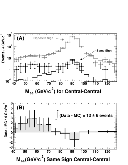
We cross-check the estimation of the dijet background for the central-central topology using same-sign events in the data sample after correcting for the contribution from charge misidentification. The dominant contribution to the charge misidentification of electrons comes from “trident” electrons except at very high energies where the curvature resolution is the dominant source (see Sec. III.6). The number of same-sign $Z/\gamma^{*}\rightarrow\ e^{+}e^{-}$ events due to “trident” electrons is estimated from the Monte Carlo simulation. The Monte Carlo samples are normalized such that the number of opposite-sign events in the $Z$ peak is the same between the data and the Monte Carlo simulation. Figure 15A shows the resulting invariant-mass distributions in data and Monte Carlo simulation for opposite-sign events and same-sign events. The number of same-sign events is found to be 36 in the data and 23 in the simulation, resulting in the estimation of 13 dijet background events for the central-central topology. Figure 15B shows the invariant-mass distribution for the same-sign data events after the Monte Carlo same-sign events are subtracted. A systematic uncertainty of 4 events is estimated by repeating this procedure with the Monte Carlo samples generated with various amounts of material. Hence the dijet background in the central-central topology is estimated to be $13\pm 6{\rm(stat.)}\pm 4{\rm(syst.)}$ events. This is in good agreement with the estimate obtained from the fake-rate method of $9.0\pm 3.2$ events.

Figure 15: (A) invariant-mass distributions of data (points) and Monte Carlo events (histogram) in the central-central topology where the Monte Carlo sample is normalized to the data using opposite-sign events in the $Z$ peak. (B) invariant-mass distribution of same-sign data in the central-central topology after subtracting the same-sign MC distribution. The Monte Carlo subtracted same-sign distribution in (B) is a measurement of the dijet background.

IV.2 Electroweak and top backgrounds

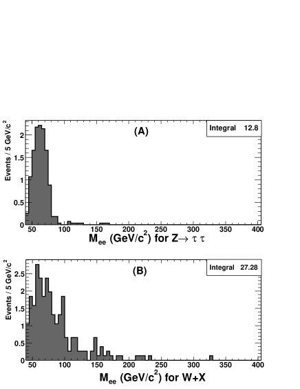
The electroweak and top background events are estimated using the Monte Carlo simulation. Table 7 shows the theoretical cross section and the number of events expected in the sample of 72 pb^-1 for each process. The systematic uncertainties on these background estimates reflect the 6% uncertainty on the integrated luminosity, the 5% uncertainty on the acceptances, and the uncertainties on the theoretical production cross sections. The simulated events for each process which pass the selection requirements are used to determine both the invariant-mass distributions and the expected forward-backward asymmetries. The invariant-mass distributions for $Z\rightarrow\tau^{+}\tau^{-}$ and $W+X\rightarrow e\nu+X$ are shown in Fig. 16.

The dominant electroweak background comes from the $W+X\rightarrow e\nu+X$ process where $X$ is a photon or hadronic jet and the $Z/\gamma^{*}\rightarrow\ \tau^{+}\tau^{-}$ process where $\tau\rightarrow e\nu_{\tau}\nu_{e}$. While the $\mbox{$Z/\gamma^{*}\rightarrow\ \tau^{+}\tau^{-}$}\rightarrow\mbox{$e^{+}e^{-}$}\nu_{\tau}\nu_{e}\bar{\nu}_{\tau}\bar{\nu}_{e}$ background is reliably simulated by LO-based generators such as PYTHIA, the $W+X\rightarrow e\nu+X$ background estimated from PYTHIA requires cross-checks with the next-to-leading order (NLO) calculations. PYTHIA, using the parton-shower algorithms to generate photons and jets, is expected to give lower cross sections than the Standard Model prediction for high-$p_{{}_{T}}$ photons and jets. We cross-check the PYTHIA calculation with two matrix-element calculations, ALPGEN for $W$ + 1 parton production and WGAMMA for $W$ + 1 photon production. The number of $W+X\rightarrow e\nu+X$ background events estimated from PYTHIA is $27\pm 5$. The combination of ALPGEN and WGAMMA estimates this number to be $24\pm 3$, in good agreement with the PYTHIA expectation within the statistical uncertainties. The difference between the PYTHIA and the ALPGEN/WGAMMA estimates is used as a systematic uncertainty on $A_{FB}$. Table 3 shows the sources of the electron candidates in the PYTHIA $W+X$ sample, indicating that the dominant source is from photons faking an electron (mostly in the plug region).

Process	$\sigma\cdot BR$ (pb)	Events Expected
		C-C	C-P
Dijet	N/A	$9.0\pm 3.2$	$128\pm 45$
$W+jet/\gamma\rightarrow e\nu+jet/\gamma$	$2,690\pm 100$	$1.8\pm 0.2$	$25.4\pm 2.4$
$Z/\gamma^{*}\rightarrow\tau^{+}\tau^{-}$	$252\pm 9$	$5.6\pm 0.5$	$7.2\pm 0.7$
$W^{+}W^{-}\rightarrow e^{+}e^{-}\nu_{e}\bar{\nu}_{e}$	$0.15\pm 0.01$	$1.5\pm 0.1$	$1.8\pm 0.2$
$W^{\pm}Z$ where $Z\rightarrow\ e^{+}e^{-}$	$0.15\pm 0.01$	$1.4\pm 0.1$	$1.7\pm 0.2$
$\mbox{$t\overline{t}$}\rightarrow\mbox{$e^{+}e^{-}$}\nu\bar{\nu}+\mbox{$b\overline{b}$}$	$0.08\pm 0.01$	$1.1\pm 0.1$	$0.7\pm 0.1$

Table 7: Summary of expected backgrounds. Cross sections for the electroweak and top processes are taken from the following references: Hamberg et al. (1991); Harlander and Kilgore (2002) for $W$ and $Z$, Campbell and Ellis (1999) for $W^{+}W^{-}$ and $WZ$, and Cacciari et al. (2004); Bonciani et al. (1998); Catani et al. (1996) for $t\bar{t}$. Monte Carlo estimates are normalized to $72$ pb^-1.

Figure 16: Invariant-mass distributions for (A) $Z/\gamma^{*}\rightarrow\ \tau^{+}\tau^{-}$ and (B) $W+X\rightarrow e\nu+X$ ($X=q,g$ or $\gamma$) backgrounds.

V Acceptance and corrections

In order to correct the raw forward-backward asymmetry measured in $Z/\gamma$ decays and obtain $A_{FB}^{phys}$, this analysis must account for any acceptances and detector effects that can change the number of forward and backward events found in each $M_{ee}$ bin. Although there is very little in the detector and analysis that treats forward and backward events differently, the angular distribution of the events, radiation, and detector resolution can each effectively change event acceptances and the reconstructed invariant mass so that net differences arise for forward and backward events. The dominant contributions to the detector acceptances are kinematic acceptance ($a_{kin}^{\pm}$), geometric acceptance ($a_{geom}^{\pm}$), and electron identification efficiency ($\epsilon_{ID}^{\pm}$). The major effects that contribute to event migration between $M_{ee}$ bins are the energy resolution of the detector ($a_{res}^{\pm}$), and internal and external bremsstrahlung ($a_{rad}^{\pm}$). Although the simulation is ultimately used to determine the corresponding corrections, generator-level distributions are used to separate and understand the various effects (Secs. V.1, V.2, and V.3). These studies assume the Standard Model $A_{FB}$ distribution from PYTHIA, and are included to demonstrate how the acceptance and detector effects independently change $A_{FB}^{raw}$.

We present two unfolding methods to reconstruct $A_{FB}^{phys}$. In Sec. V.4, the simulation is used to find a parameterization to transform $A_{FB}^{phys}$ into $A_{FB}^{raw}$. This parameterization is used to determine the $A_{FB}^{phys}$ that corresponds to our measured $A_{FB}^{raw}$. In Sec. V.5, correction factors are calculated which transform the number of forward and backward events in the candidate sample to the number of forward and backward events that existed prior to being degraded by detector acceptances and $M_{ee}$ bin migration. The bias from the input $A_{FB}^{phys}$ on the correction factor calculation is also discussed. Both unfolding analyses assume the Standard Model $\frac{d\sigma}{dM_{ee}}$ to be able to calculate the event migration effects.

V.1 Fiducial and kinematic acceptance: $a^{\pm}_{geom}$ and $a^{\pm}_{kin}$

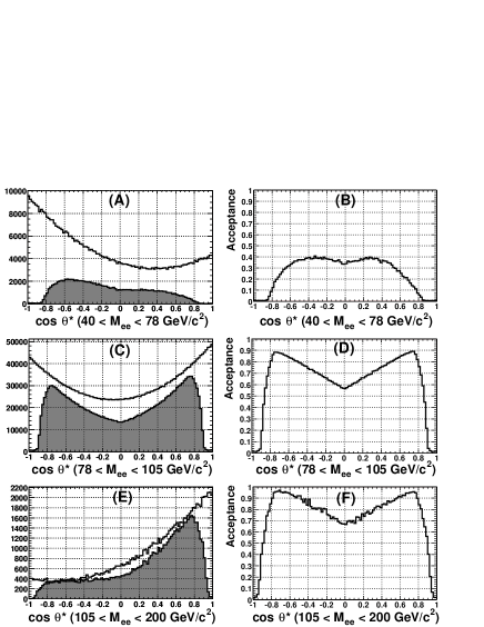
The kinematic and fiducial event requirements sculpt the polar angular distribution of the outgoing electrons and positrons, especially at high $|\mbox{$\cos\theta^{*}$}|$. The distributions in Fig. 17 show this effect for Monte Carlo events prior to the simulation of detector and radiation effects. The invariant-mass range is split into three different regions, the low-mass region ($40<\mbox{$M_{ee}$}<78$ GeV/$c^{2}$), the $Z$ pole region ($78<\mbox{$M_{ee}$}<105$ GeV/$c^{2}$), and the high-mass region ($M_{ee}>105$ GeV/$c^{2}$). These are the regions where $A_{FB}$ is roughly at the low extremum, middle point, and high extremum, respectively. Although the acceptance for these requirements is nearly symmetric for positive and negative $\cos\theta^{*}$, the initial $\cos\theta^{*}$ distributions are asymmetric, due to the forward-backward charge asymmetry. When integrating the positive and negative portions of $\cos\theta^{*}$, the convolution of the Drell-Yan spectrum with the acceptance gives a different total acceptance for forward and backward events. For example, the detector has a low acceptance for events with very high $|\mbox{$\cos\theta^{*}$}|$ because of the polar coverage, and in the case of high-mass events, this removes a greater percentage of forward events than backward events (see Fig. 17E). The $M_{ee}$ dependence of the fiducial and kinematic acceptance is shown in Figs. 18A and 18B, where the forward events have a higher acceptance than the backward events below the $Z$ pole, and vice versa above the $Z$ pole.

Figure 17: For three mass ranges, the $\cos\theta^{*}$ distributions (A, C, E) before (open histograms) and after (filled histograms) the geometric and kinematic cuts; and the acceptance, $a^{\pm}_{geom}\cdot a^{\pm}_{kin}$, as a function of $\cos\theta^{*}$ (B, D, F).

Figure 18: The $M_{ee}$ dependence of acceptances; $a^{\pm}_{geom}$ (A), $a^{\pm}_{kin}$ (B), $a^{\pm}_{res}$ (C), and $a^{\pm}_{rad}$ (D). The kinematic acceptance, $a^{\pm}_{kin}$, is calculated after geometric cuts are applied, the acceptance due to resolution, $a^{\pm}_{res}$, is calculated after geometric and kinematic cuts are applied, and the acceptance due to radiation, $a^{\pm}_{rad}$, is calculated after geometric and kinematic cuts and resolution smearing are applied.

V.2 Corrections for energy resolution: $a^{\pm}_{res}$

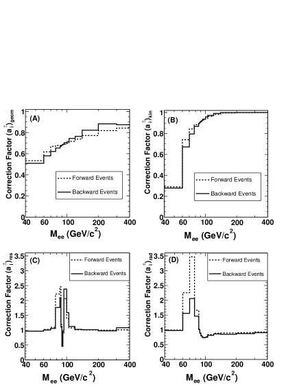
The energy resolution of the calorimeter causes mismeasurements of the invariant mass which can place events in the wrong invariant-mass bin. If the asymmetry is changing with invariant mass, events placed in the wrong invariant-mass bin alter the measured asymmetry in that bin. The effect of the energy resolution on the measured asymmetry is therefore largest near the $Z$ pole where $\frac{d\mbox{$A_{FB}$}}{d\mbox{$M_{ee}$}}$ is largest and the bin sizes are smallest. As events from the $Z$ pole are smeared out, some events move to higher masses where $A_{FB}$ is more forward, and some events move to lower masses where the $A_{FB}$ is more backward. This event migration increases the correction factor for backward events above the $Z$ pole and increases the correction factor for forward events below the $Z$ pole. The effect of the energy resolution on the correction factor is shown Fig. 18C. This plot is made by smearing the energy of the generator-level electron according to the measured detector response.

V.3 Corrections for bremsstrahlung: $a^{\pm}_{rad}$

The invariant mass can also be mis-measured due to the effects of final state bremsstrahlung. Most of these photons are emitted co-linearly with the electrons and deposit their energy into the same calorimeter towers as the electron. In these cases, the energy of the electron is recombined with its radiation products. Photons which are not recombined with electrons in the energy measurement lower the measured invariant mass and can cause a candidate event to land in the wrong invariant-mass bin. The effect is expected to be the most significant just below the $Z$ pole. Figure 18D demonstrates the effect of internal bremsstrahlung on the acceptance at the generator level (no external bremsstrahlung is included in this plot), when photons are not recombined with electrons. The correction factor below the $Z$ pole is large because of events from the $Z$ pole that are being mis-measured due to radiation. The $A_{FB}$  at the $Z$ pole is larger, and boosts the correction factor for forward events.

V.4 Parameterized acceptance and smearing

In order to transform $A_{FB}^{phys}$ into $A_{FB}^{raw}$, a parameterized function is needed to take into account the event loss and migration of events from one invariant-mass bin to another. From the Monte Carlo simulation, we compute the efficiency $\epsilon^{FF}_{ij}$ for an event that is forward and in $M_{ee}$ bin $i$ to be found in the detector as forward in bin $j$. Likewise, $15\times 15$ efficiency matrices are calculated for backward events being found as backward ($\epsilon^{BB}_{ij}$), forward as backward ($\epsilon^{FB}_{ij}$), and backward as forward ($\epsilon^{BF}_{ij}$). So the diagonal elements of $\epsilon^{FF}$ and $\epsilon^{BB}$ approximately represent the acceptance for events in those bins, and the off-diagonal elements approximately represent the event bin migration. The elements of $\epsilon^{BF}$ and $\epsilon^{FB}$ are much smaller and represent those events that are reconstructed with a $\cos\theta^{*}$ of the wrong sign. These efficiencies have a small dependence on the underlying $\cos\theta^{*}$ distribution, and so there is some residual dependence on the input $A_{FB}^{phys}$ used to calculate them. This might have a small bias on the result if the $\cos\theta^{*}$ distribution in the data is very different from the Standard Model. In Sec. VII.1, the $\cos\theta^{*}$ distribution shows very good agreement between data and the Standard Model prediction. The four matrices are defined as

$$\epsilon^{FF}_{ij} = {\frac{N^{F}_{j}(sel)}{N^{F}_{i}(gen)}}~{};~{}\epsilon^{BB}_{ij}={\frac{N^{B}_{j}(sel)}{N^{B}_{i}(gen)}}$$ (16)

$$\epsilon^{FB}_{ij} = {\frac{N^{B}_{j}(sel)}{N^{F}_{i}(gen)}}~{};~{}\epsilon^{BF}_{ij}={\frac{N^{F}_{j}(sel)}{N^{B}_{i}(gen)}}$$ (17)

where $N^{F}_{i}(gen)~{}[N^{B}_{i}(gen)]$ is the number of forward [backward] events generated in the i-th $M_{ee}$ bin, and $(N^{F}_{i}(sel)~{}[N^{B}_{i}(sel)]$ is the number of forward [backward] events selected in the i-th $M_{ee}$ bin. By solving for $N^{F}$ or $N^{B}$ in Eq. (7), we find the expected number of forward and backward events for a given $A_{FB}$,

$$N^{F/B}_{i}(phys)={N^{tot}_{i}(phys)\cdot(0.5\pm 0.5\cdot(\mbox{$A_{FB}^{phys}$})_{i})}.$$ (18)

$N^{tot}_{i}(phys)$ is the total number of events in bin $i$, and is computed from the Standard Model $\frac{d\sigma}{dM_{ee}}$. Then by combining the expected number of events and their corresponding efficiencies, the expected number of events found in the detector is written as

$$N^{F}_{j}(raw)=\sum_{i}^{15}(\epsilon^{FF}_{ij}\cdot N^{F}_{i}(phys)+\epsilon^{BF}_{ij}\cdot N^{B}_{i}(phys))$$ (19)

$$N^{B}_{j}(raw)=\sum_{i}^{15}(\epsilon^{BB}_{ij}\cdot N^{B}_{i}(phys)+\epsilon^{FB}_{ij}\cdot N^{F}_{i}(phys))$$ (20)

For a given A or 15 $A_{FB}^{phys}$ values, $N^{F}_{j}(raw)$ and $N^{B}_{j}(raw)$ can be used together with Eq. (7) to find $(\mbox{$A_{FB}^{raw}$})_{j}$, which can be directly compared to the $A_{FB}^{raw}$ measured in the detector.

$$(\mbox{$A_{FB}^{raw}$})_{j}=g(\textbf{A},j)=\frac{N^{F}_{j}(raw)-N^{B}_{j}(raw)}{N^{F}_{j}(raw)+N^{B}_{j}(raw)}$$ (21)

V.5 Calculation of the correction factor $a^{\pm}_{cor}$

The multiplicative correction factor $(a^{+}_{cor})_{i}$ [$(a^{-}_{cor})_{i}$], used to correct $A_{FB}$ in Eq. (15), is designed to be multiplied by the number of forward [backward] events in the $i$-th $M_{ee}$ bin. It corrects for event losses and for events that migrated into bin $i$ from another bin with a different $A_{FB}$. The full simulation is used to calculate the $a^{\pm}_{cor}$ which include the effects of fiducial and kinematic acceptance, energy resolution, bremsstrahlung, and electron selection efficiency. The combination of all these effects is defined as $(a^{\pm}_{cor})_{i}$ in Eq. (V.5).

$$(a^{\pm}_{cor})_{i} = {\frac{N^{F/B}_{i}(sel)}{N^{F/B}_{i}(gen)}}$$

$$= (a^{\pm}_{geom})_{i}\cdot(a^{\pm}_{kin})_{i}\cdot(a^{\pm}_{res})_{i}\cdot(a^{\pm}_{rad})_{i}\cdot(\epsilon^{\pm}_{ID})_{i},$$

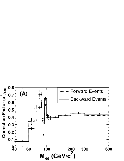
In Fig. 19A and Table 8, the resulting correction factor is shown as a function of the dielectron invariant mass. This result can be compared to the studies done at the generator level for each individual effect (see Fig. 18). The overall acceptance is lower due to the more detailed fiducial cuts and electron identification efficiencies in the full simulation. It is important to note that the correction for event migration depends on the input $A_{FB}^{phys}$ assumption used to calculate $(a^{\pm}_{cor})_{i}$. The correction can only be calculated by assuming the difference in $A_{FB}^{phys}$ between the bin being corrected and the bins from which the events migrated. If the $A_{FB}^{phys}$ is significantly different in the two bins and there is a large amount of event migration, the result of the correction can be biased by this assumption.

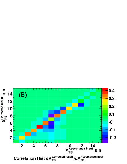
To measure the bias of the input $A_{FB}$ on the final result, the correlation matrix ($\frac{dA_{FB}^{\rm{Corrected~{}result}}}{dA_{FB}^{\rm{Acceptance~{}Input}}}$) is measured by separately reweighting the input $A_{FB}$ in each bin in the Monte Carlo sample used to calculate the correction factor. The modified correction factors are then used to correct the $A_{FB}$ from a high-statistics pseudo-experiment using Eq. (15), and the change in the $A_{FB}$ result in each $M_{ee}$ bin is measured relative to the change in the input $A_{FB}$ (Fig. 19B). The lowest mass bin and four highest mass bins are fairly independent of the $A_{FB}^{phys}$ used to calculate the acceptance, whereas the bins near the $Z$ pole have strong correlations.

To minimize the bias, one of the results uses the $A_{FB}^{phys}$ from Sec. VII.4, calculated using Standard Model constraints, as the input to the $(a^{\pm}_{cor})_{i}$ calculation. In this approach, the uncertainties on the input $A_{FB}^{phys}$ from the coupling fits are taken as systematic uncertainties on the acceptance measurement.

Figure 19: The correction factors, $a^{\pm}_{cor}$ (A). The input $A_{FB}^{phys}$ is taken from the $A_{FB}$ couplings fit (Sec. VII.4). The correlation matrix between the input $A_{FB}^{phys}$ to the correction factor calculation and the corresponding change in the result due to Eq. (15) (B). The axes are labeled by the $M_{ee}$ bin number where bin 1 is the lowest mass bin (40$<\mbox{$M_{ee}$}<$60 GeV/$c^{2}$), bin 15 is the highest mass bin (300$<\mbox{$M_{ee}$}<$600 GeV/$c^{2}$), and bin 7 is the $Z$ pole (90$<\mbox{$M_{ee}$}<$92 GeV/$c^{2}$).

Mass Range	Forward	Backward
$40<M_{ee}<60$ GeV/c2	0.08 $\pm$ 0.00	0.07 $\pm$ 0.00
$60<M_{ee}<70$ GeV/c2	0.34 $\pm$ 0.05	0.25 $\pm$ 0.01
$70<M_{ee}<78$ GeV/c2	0.53 $\pm$ 0.05	0.36 $\pm$ 0.01
$78<M_{ee}<86$ GeV/c2	0.72 $\pm$ 0.06	0.53 $\pm$ 0.02
$86<M_{ee}<88$ GeV/c2	0.72 $\pm$ 0.03	0.60 $\pm$ 0.02
$88<M_{ee}<90$ GeV/c2	0.39 $\pm$ 0.01	0.35 $\pm$ 0.00
$90<M_{ee}<92$ GeV/c2	0.16 $\pm$ 0.00	0.16 $\pm$ 0.00
$92<M_{ee}<94$ GeV/c2	0.31 $\pm$ 0.00	0.33 $\pm$ 0.00
$94<M_{ee}<100$ GeV/c2	0.56 $\pm$ 0.01	0.65 $\pm$ 0.02
$100<M_{ee}<105$ GeV/c2	0.39 $\pm$ 0.00	0.43 $\pm$ 0.01
$105<M_{ee}<120$ GeV/c2	0.37 $\pm$ 0.00	0.40 $\pm$ 0.00
$120<M_{ee}<140$ GeV/c2	0.39 $\pm$ 0.00	0.40 $\pm$ 0.01
$140<M_{ee}<200$ GeV/c2	0.42 $\pm$ 0.00	0.43 $\pm$ 0.01
$200<M_{ee}<300$ GeV/c2	0.45 $\pm$ 0.00	0.45 $\pm$ 0.01
$300<M_{ee}<600$ GeV/c2	0.42 $\pm$ 0.00	0.43 $\pm$ 0.01

Table 8: The correction factors, $a^{\pm}_{cor}$, for the different mass bins using $A_{FB}$ from the Standard Model coupling fits of Sec. VII.4.

VI Systematic uncertainties in $A_{FB}$

Systematic uncertainties due to energy scale, energy resolution, the amount of passive material in the detector, and background estimation are considered. For a given source of uncertainty, a change is made to the corresponding parameter in the simulation, and the impact on the asymmetry is evaluated after that change. The difference between the asymmetry with the changed parameter and the nominal one is taken as the uncertainty from that source. The change in the input parameter is either a one standard deviation (1$\sigma$) uncertainty on the variable in question or a change in an assumption on that input. The systematic uncertainties depend on the method that is used to extract $A_{FB}^{phys}$. There are separate tables for the systematic uncertainty on $A_{FB}^{phys}$ for the two $A_{FB}$ measurements (Tables 9 and 10). The $A_{FB}$ measurement based on the $a^{\pm}_{cor}$ correction factors has an additional uncertainty due to the Standard Model assumptions used the calculate these factors (see Table 10). The systematic uncertainties are quoted with a sign that represents the sign of the change in $A_{FB}$ due to the $+1\sigma$ variation and is not used in the measurement of $A_{FB}$. A positive variation represents an increase in the energy scale and resolution, an increase in the amount of material, and an increase in the amount of background.

The following systematic uncertainties have been investigated and have been found to have negligible effects on the measurement of $A_{FB}$: fiducial acceptance, charge misidentification, $A_{FB}$(dijet), and trigger efficiency. These effects are not included in the total systematic uncertainty.

VI.1 Systematic uncertainty from energy scale

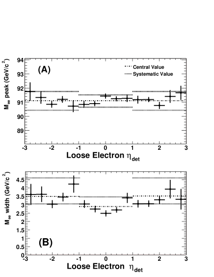
Variations in the calorimeter energy scale can lead to events being placed in the wrong invariant-mass bins. For example, near the $Z$ pole where the asymmetry is increasing monotonically with respect to the invariant mass, a positive variation in the energy scale will cause a systematic decrease in the asymmetry (or a systematic increase for a negative variation in the energy scale). In general, a variation in the energy scale will have an effect only in the region where the bins are of the same order as the size of the variations (or smaller) and where the asymmetry is changing. In this analysis, uncertainties due to the energy scale are expected only in the region near the $Z$ pole. Figure 20 shows the Gaussian peak of the invariant mass as a function of the $\eta_{det}$ of the electron. Based on the distribution of calculated masses, the central calorimeter scale is varied by 0.5% and the plug calorimeter scale is varied by 1% to estimate the systematic uncertainties. The chosen energy scale variations are shown as lines in Fig. 20. The corresponding shifts in $A_{FB}$ are shown in Tables 9 and 10.

Figure 20: The peak (A) and width (B) of a Gaussian fit to the $M_{ee}$ peak between 86 and 98 GeV/$c^{2}$ as a function of $\eta_{det}$ of loose electrons. The points are the data, and the lines are the chosen variations in the energy scale and resolution used to estimate the systematic uncertainties.

VI.2 Systematic uncertainty from energy resolution

Variations in the energy resolution impact the forward-backward charge asymmetry in much the same way as variations in the energy scale. Instead of systematically shifting the events upwards or downwards, they tend to smear the forward-backward charge asymmetry to an average of the bins around the bin in question. For example, a positive variation in the resolution near the $Z$ peak will cause a systematic decrease in the measured asymmetry above the $Z$ peak and a systematic increase in the asymmetry below the $Z$ peak. As in the case of the energy scale, only narrow bins in the region where the $\frac{d\mbox{$A_{FB}$}}{d\mbox{$M_{ee}$}}$ is large will be affected. Figure 20 shows the Gaussian width of the invariant mass as a function of the $\eta_{det}$ of the electron. Based on the distribution of the widths, the central and plug calorimeter resolutions varied by 0.5 GeV in the central calorimeter and 1.5 GeV in the plug calorimeter. In the central calorimeter, only the change due to increasing the resolution is used in calculating the systematic. The chosen variations are shown as lines in Fig. 20. The corresponding shifts $A_{FB}$ are shown in Tables 9 and 10.

VI.3 Systematic uncertainty from amount of material

The amount of material in front of the calorimeter affects the energy measurement of electrons. The uncertainty in the amount of material is estimated to be less than 1.5% of a radiation length ($X_{0}$) in the region between the interaction point and the tracking volume, and less than ${\frac{1}{6}}X_{0}$ in the region between the collision point and the plug calorimeter.

The systematic uncertainty on $A_{FB}$ due to the material is estimated by changing the amount of material in the simulation. The changes include adding or subtracting an extra $1.5\%X_{0}$ of copper in a cylinder at 34 cm (just before the COT) and ${\frac{1}{6}}X_{0}$ of steel on the face of the plug calorimeter. The corresponding shifts in $A_{FB}$ are shown in Tables 9 and 10. The bins most sensitive to the amount of material are those just below the $Z$ pole; this is more easily seen in the systematics on the fit result (Table 9).

VI.4 Systematic uncertainty from background subtraction

The central values of $A_{FB}$ are calculated after subtracting background events in the forward and backward regions separately. The number of background events in each $M_{ee}$ bin are estimated in Sec. IV. The systematic uncertainties due to the background estimates are taken as shifts in $A_{FB}$ when the estimated numbers of background events are varied by their uncertainties. The corresponding shifts $A_{FB}$ are shown in Tables 9 and 10.

Mass Range	Energy	Energy	Material	Bgrnd	Tot	Stat
(GeV/$c^{2}$)	Scale	Resol.
$40-60$	-0.003	0.010	-0.035	-0.034	0.050	0.127
$60-70$	0.008	0.008	0.033	-0.065	0.074	0.185
$70-78$	-0.018	0.019	0.040	-0.017	0.051	0.186
$78-86$	0.037	0.064	-0.041	0.001	0.085	0.164
$86-88$	-0.080	0.112	0.135	-0.001	0.193	0.211
$88-90$	-0.072	-0.032	0.043	-0.000	0.090	0.108
$90-92$	0.058	0.042	-0.024	0.000	0.076	0.064
$92-94$	-0.118	-0.098	0.049	0.000	0.161	0.161
$94-100$	0.031	-0.077	0.013	0.000	0.084	0.168
$100-105$	-0.046	-0.146	-0.103	-0.000	0.185	0.258
$105-120$	-0.001	0.014	0.045	0.014	0.049	0.138
$120-140$	-0.003	-0.004	-0.003	-0.001	0.006	0.185
$140-200$	0.002	0.003	0.012	0.004	0.013	0.165
$200-300$	-0.005	-0.007	0.006	0.026	0.029	${}^{+0.20}_{-0.27}$
$300-600$	-0.004	0.002	-0.023	0.000	0.024	${}^{+0.00}_{-0.51}$

Table 9: Sources of systematic uncertainty, the total systematic uncertainty (Tot), and the statistical uncertainty (Stat) on $A_{FB}^{phys}$ when fitting using the parameterization described in Sec. V.4 (see Sec. VII.3). When a systematic shift is tested in two directions ($+1\sigma$ and $-1\sigma$ of the variable in question), the larger shift is chosen. The sign represents the sign of the change in $A_{FB}$ due to the $+1\sigma$ variation and is not used in the measurement of $A_{FB}$.

Mass Range	Energy	Energy	Material	Bgrnd	Input	Tot	Stat
(GeV/$c^{2}$)	Scale	Resol.
$40-60$	-0.013	0.013	-0.028	-0.053	-0.018	0.065	0.108
$60-70$	0.012	0.012	0.027	-0.038	0.074	0.089	0.095
$70-78$	-0.010	0.014	-0.022	-0.009	-0.041	0.050	0.072
$78-86$	-0.015	0.033	0.012	-0.001	-0.053	0.066	0.043
$86-88$	-0.013	0.015	0.013	0.001	-0.034	0.041	0.048
$88-90$	-0.011	0.005	0.011	-0.000	-0.014	0.021	0.035
$90-92$	0.006	0.006	-0.009	0.001	0.009	0.015	0.031
$92-94$	-0.009	-0.005	-0.010	0.000	-0.004	0.014	0.033
$94-100$	-0.014	-0.022	-0.010	0.000	-0.017	0.033	0.034
$100-105$	-0.017	-0.080	-0.045	0.002	-0.015	0.095	0.099
$105-120$	-0.013	-0.014	0.027	0.011	-0.004	0.035	0.091
$120-140$	-0.004	-0.004	0.008	0.023	-0.008	0.026	${}^{+0.14}_{-0.15}$
$140-200$	0.004	0.004	0.011	0.006	-0.007	0.016	${}^{+0.14}_{-0.15}$
$200-300$	-0.008	-0.008	0.017	0.033	-0.005	0.039	${}^{+0.18}_{-0.24}$
$300-600$	-0.017	0.017	-0.032	0.000	0.000	0.040	${}^{+0.00}_{-0.64}$

Table 10: Summary of uncertainties on $A_{FB}^{phys}$ calculated using Eq. (15) and the couplings fits for $A_{FB}$ as input to the acceptance calculation. When a systematic shift is tested in two directions ($+1\sigma$ and $-1\sigma$ of the variable in question), the larger shift is chosen. The sign represents the sign of the change in $A_{FB}$ due to $+1\sigma$ variation and is not used in the measurement of $A_{FB}$. The systematic uncertainty due to the Standard Model assumptions used in the correction factor calculation is labeled as “Input.”

VII Results

VII.1 Comparisons of uncorrected distributions with the Standard Model

The best way to make a direct comparison of the data with the Standard Model is to use the simulation to compare the uncorrected data with simulated events. The background events are included using the predicted distributions as described in Sec. IV. The distributions from the signal Monte Carlo simulation are normalized to the number of events in the data after subtracting the predicted background contribution. Only statistical uncertainties have been included for the calculation of the $\chi^{2}$ comparisons. The uncorrected invariant-mass distribution from the data is compared to the signal and background predictions in Fig. 21. Since the energy scale and resolution in the simulation has been tuned to the data at the $Z$ peak (Sec. III.5), the comparison of the $M_{ee}$ lineshape gives a slightly better than expected $\chi^{2}$/DOF=26.7/35. The comparison is also made for the $\cos\theta^{*}$ distribution (Fig. 22) in three mass regions where $A_{FB}$ is at extremes; $40<\mbox{$M_{ee}$}<75$ GeV/$c^{2}$ where $A_{FB}$ is large and negative (giving a $\chi^{2}$/DOF=9.9/9), $75<\mbox{$M_{ee}$}<105$ GeV/$c^{2}$ where $A_{FB}$ is small (giving $\chi^{2}$/DOF=44.8/39), and $\mbox{$M_{ee}$}>105$ GeV/$c^{2}$ where $A_{FB}$ is large and positive (giving $\chi^{2}$/DOF=7.8/9). Finally, the comparison of $A_{FB}^{raw}$ in 15 $M_{ee}$ bins (Table 11) with the Standard Model simulation gives a $\chi^{2}$/DOF=15.7/15. The data shows excellent agreement with the Standard Model in all of these distributions. The objective of the following sections will be to obtain the corrected $A_{FB}^{phys}$ and $Z$ couplings that can be used without the CDF simulation.

Figure 21: Invariant-mass distribution of the data compared to the prediction for signal and background combined. The points are the data, the histogram is the signal Monte Carlo sample, and the shaded histograms are the background predictions. The contributions are added or stacked.

Figure 22: Distributions of $\cos\theta^{*}$ for the three mass regions of the data compared to the predictions for the signal and background combined. The points are the data, the open histograms are the predictions from signal Monte Carlo simulation, and the shaded histograms are the predictions from background. The contributions are added or stacked.

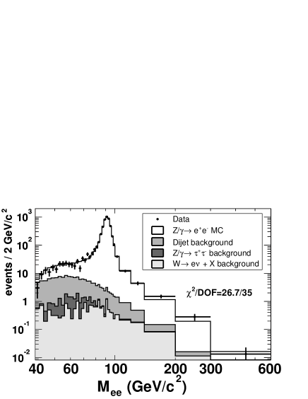
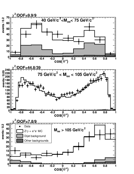
VII.2 The Standard Model prediction

Currently, there are a number of programs that generate Drell-Yan events produced in hadron collisions. PYTHIA generates events using leading-order (LO) cross sections and incorporates initial-state QCD radiation and initial- and final-state QED radiation via parton shower algorithms. HERWIG uses LO cross sections with initial state QCD radiation via parton shower algorithms. ZGRAD Baur et al. (2002) includes full $\mathcal{O}(\alpha)$ electroweak corrections but no QCD corrections, resulting in $p_{T}^{Z/\gamma*}\simeq 0$. The gluon resummation program VBP Ellis and Veseli (1998); Ellis et al. (1997), which does the gluon resummation in the $q_{t}$ space at low $p_{T}^{Z/\gamma*}$ and reduces to NLO QCD at high $p_{T}^{Z/\gamma*}$, does not include any electroweak corrections. Unfortunately, there is no one program that includes both $\mathcal{O}(\alpha)$ electroweak and NLO QCD corrections. A calculation that includes $\mathcal{O}(\alpha)$ electroweak and some QCD corrections can be obtained by running ZGRAD with the parton showering code in PYTHIA. Six Monte Carlo programs are used to constrain the possible values for the $A_{FB}$ measurement. They are PYTHIA, VBP, ZGRAD, ZGRAD + PYTHIA, and PYTHIA with no QCD corrections with CTEQ5L parton distribution functions, and PYTHIA with MRST2001 parton distribution functions. In each mass bin, a band is constructed to extend from the lowest to the highest values of the six $A_{FB}$ calculations. The uncertainty on the theoretical prediction due to different event generators is taken to be the width of the band in any mass bin. In Fig. 23, each calculation is compared to the center and width of the band in each $M_{ee}$ bin. A comparison of these Monte Carlo programs also demonstrates the extent to which the Collin-Soper frame (Sec. II.4) minimizes the impact of the transverse momentum of the incoming quarks. The PYTHIA (LO) and ZGRAD programs, which have no initial-state QCD radiation, can be compared to the VBP, ZGRAD+PYTHIA, and PYTHIA programs which include initial-state QCD radiation. The difference in $A_{FB}$ between having and not having initial-state QCD radiation is negligible compared to the $A_{FB}$ measurement uncertainties (see Fig. 24).

Figure 23: Each of six theoretical calculations compared to the center and width of the theoretical band. The variation from different theoretical calculations is expressed as the width of the band which is determined by the highest and lowest values of $A_{FB}$, including the uncertainties, in each mass bin.

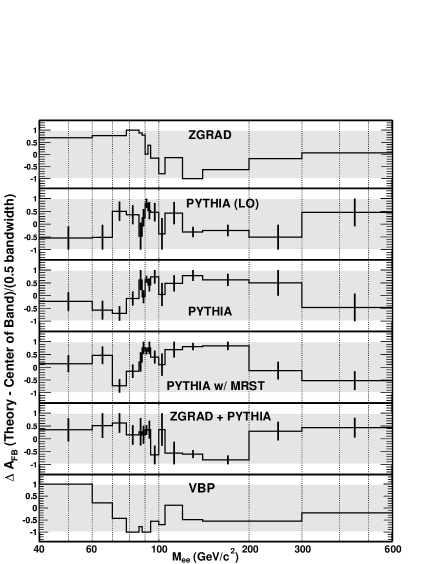
VII.3 $A_{FB}$ measurement without Standard Model constraints

The forward-backward charge asymmetry is measured using the maximum likelihood method and comparing $A_{FB}^{raw}$ returned by the parameterized acceptance and smearing from Sec. V.4 to the data at detector level. This method is unbiased since it does not make any prior assumption about the values of $A_{FB}$. The number of events in various invariant-mass bins between 40 GeV/$c^{2}$ and 600 GeV/$c^{2}$ and $A_{FB}^{raw}$ are summarized in Table 11.

The probability for finding a forward or backward event for a given $A_{FB}$ is

$$P(^{F}_{B}) = {\frac{1}{2}(1\pm\mbox{$A_{FB}$})},$$ (23)

and the probability to find $N^{F}$ forward and $N^{B}$ backward events among $N$ events is given by the binomial distribution:

$$P(\mbox{$A_{FB}$},N^{F},N^{B})= {(^{N}_{N^{F}})\cdot(1+\mbox{$A_{FB}$})^{N^{F}}}$$ (24)

$${\cdot(1-\mbox{$A_{FB}$})^{N^{B}}\cdot(\frac{1}{2})^{N^{F}+N^{B}}}.$$

Defining $\alpha$ as the negative logarithm of the likelihood function, we obtain:

$$\alpha=\sum_{i}^{15} -N_{i}^{F}\cdot log(1+g(\textbf{A},i))$$ (25)

$$-N_{i}^{B}\cdot log(1-g(\textbf{A},i))+C,$$

$$\mathrm{where}~{}{\textbf{A}}=\{(\mbox{$A_{FB}^{phys}$})_{1},(\mbox{$A_{FB}^{phys}$})_{2},\ldots,(\mbox{$A_{FB}^{phys}$})_{15}\}.$$ (26)

The large correlations between invariant-mass bins near the $Z$ pole (see Fig. 19B) lead to large uncertainties on $A_{FB}$. In this case, it is customary to add a regularization function to the likelihood Cowan (2002) to reduce the variances. We choose the Tikhonov regularization, which adds a function proportional to the second derivative of the true distribution.

$$S[\textbf{A}_{i}]={\int_{bin~{}i}\left(\frac{d^{2}f_{true}(M_{ee},\textbf{A}_{i})}{dM^{2}_{ee}}\right)^{2}dM_{ee}},$$ (27)

$$\mathrm{where}~{}{\textbf{A}}_{i}=\{(\mbox{$A_{FB}^{phys}$})_{i-1},(\mbox{$A_{FB}^{phys}$})_{i},(\mbox{$A_{FB}^{phys}$})_{i+1}\},$$ (28)

and where the integral is performed over the entire range of bin $i$ in $M_{ee}$. Since the binning is not uniform, a parabolic form is assumed for $f_{true}(M_{ee},\textbf{A}_{i})$,

$$f_{true}(M_{ee},\textbf{A}_{i})=a+b\cdot\mbox{$M_{ee}$}+c\cdot M^{2}_{ee}.$$ (29)

The parameters $a$, $b$, and $c$ are solved for by integrating $f$ over bins $i-1$, $i$, and $i+1$, and setting the integrals equal to $\textbf{A}_{i}$. $S[\textbf{A}_{i}]$ can then be simplified to

$$S[\textbf{A}_{i}]=4\cdot(c(\textbf{A}_{i}))^{2}\cdot\Delta M^{i}_{ee}.$$ (30)

This function is only applied to bins 2 through 9, since those are the bins with large migration. Adding this to the likelihood, a new equation is made

$$\alpha^{\prime}={\sum_{i=1}^{15}\{-N_{i}^{F}\cdot log(1+g(\textbf{A},i))-N_{i}^{B}\cdot log(1-g(\textbf{A},i))\}+\lambda\cdot\sum_{i=2}^{9}S[{\textbf{A}}_{i}]+C.}$$ (31)

The parameter $\lambda$ is called the regularization parameter, and is arbitrary. A very small $\lambda$ will have no effect on the fit, and a very large $\lambda$ will dominate the likelihood. In this analysis $\lambda$ is chosen such that $\alpha^{\prime}=\alpha+\frac{1}{2}$. The result is not sensitive to changes as large as a factor of 2 or $\frac{1}{2}$ in $\lambda$. The fitting package Minuit James and Roos (1975) is used to minimize $\alpha^{\prime}$, as a function of A. $A_{FB}^{phys}$ obtained after Tikhonov regularization is shown in Fig. 24 and in Table 12 for different invariant-mass bins. The statistical and systematic uncertainties of the measurement and the prediction from PYTHIA are also given in Table 12.

Mass Range	Observed Events		Background		$A_{FB}^{raw}$
(GeV/$c^{2}$)	$\mbox{$\cos\theta^{*}$}>0$	$\mbox{$\cos\theta^{*}$}<0$	$\mbox{$\cos\theta^{*}$}>0$	$\mbox{$\cos\theta^{*}$}<0$	$\pm$stat $\pm$ sys.
$40<M_{ee}<60$	76	78	37.8 $\pm$ 9.2	32.4 $\pm$ 9.2	-0.09 $\pm$ 0.11 $\pm$ 0.05
$60<M_{ee}<70$	46	68	19.0 $\pm$ 4.6	17.4 $\pm$ 4.6	-0.31 $\pm$ 0.11 $\pm$ 0.04
$70<M_{ee}<78$	69	98	12.4 $\pm$ 2.8	9.9 $\pm$ 2.7	-0.22 $\pm$ 0.08 $\pm$ 0.01
$78<M_{ee}<86$	267	266	8.2 $\pm$ 2.0	7.4 $\pm$ 2.0	0.00 $\pm$ 0.04 $\pm$ 0.00
$86<M_{ee}<88$	246	204	1.4 $\pm$ 0.4	1.6 $\pm$ 0.4	0.09 $\pm$ 0.05 $\pm$ 0.00
$88<M_{ee}<90$	420	393	1.5 $\pm$ 0.4	1.3 $\pm$ 0.3	0.03 $\pm$ 0.04 $\pm$ 0.00
$90<M_{ee}<92$	550	476	1.8 $\pm$ 0.4	1.4 $\pm$ 0.4	0.07 $\pm$ 0.03 $\pm$ 0.00
$92<M_{ee}<94$	481	392	1.4 $\pm$ 0.3	1.3 $\pm$ 0.3	0.10 $\pm$ 0.03 $\pm$ 0.00
$94<M_{ee}<100$	463	325	4.1 $\pm$ 0.9	3.1 $\pm$ 0.8	0.18 $\pm$ 0.04 $\pm$ 0.00
$100<M_{ee}<105$	59	39	2.0 $\pm$ 0.5	1.6 $\pm$ 0.5	0.21 $\pm$ 0.10 $\pm$ 0.00
$105<M_{ee}<120$	67	23	4.1 $\pm$ 0.9	3.2 $\pm$ 0.9	0.52 $\pm$ 0.09 $\pm$ 0.01
$120<M_{ee}<140$	29	15	2.2 $\pm$ 0.6	2.2 $\pm$ 0.6	0.35 $\pm$ 0.15 $\pm$ 0.02
$140<M_{ee}<200$	29	16	3.2 $\pm$ 0.6	1.9 $\pm$ 0.4	0.29 $\pm$ 0.15 $\pm$ 0.01
$200<M_{ee}<300$	11	3	0.6 $\pm$ 0.2	0.5 $\pm$ 0.2	0.61 $\pm$ 0.22 $\pm$ 0.03
$300<M_{ee}<600$	2	0	0.2 $\pm$ 0.1	0.0 $\pm$ 0.0	1.00${}^{+0}_{-0.632}$ $\pm$ 0.00

Table 11: Summary of observed events, estimated backgrounds, and $A_{FB}^{raw}$ in the dielectron sample from 72 pb^-1 of Run II data. The systematic uncertainty on $A_{FB}^{raw}$ includes only the background subtraction.

Mass Range	$<M_{ee}>$	Measured $A_{FB}$	PYTHIA $A_{FB}$
(GeV/$c^{2}$)	(GeV/$c^{2}$)
$40\leq\mbox{$M_{ee}$}<60$	48.2	-0.11 $\pm$ 0.13 $\pm$ 0.05	-0.214 $\pm$ 0.003
$60\leq\mbox{$M_{ee}$}<70$	64.9	-0.51${}^{+0.18}_{-0.17}$ $\pm$ 0.07	-0.420 $\pm$ 0.005
$70\leq\mbox{$M_{ee}$}<78$	74.3	-0.45 $\pm$ 0.19 $\pm$ 0.05	-0.410 $\pm$ 0.005
$78\leq\mbox{$M_{ee}$}<86$	83.0	-0.11 $\pm$ 0.17 $\pm$ 0.09	-0.214 $\pm$ 0.003
$86\leq\mbox{$M_{ee}$}<88$	87.1	0.07 $\pm$ 0.23 $\pm$ 0.19	-0.079 $\pm$ 0.004
$88\leq\mbox{$M_{ee}$}<90$	89.2	0.03 $\pm$ 0.13 $\pm$ 0.09	-0.001 $\pm$ 0.002
$90\leq\mbox{$M_{ee}$}<92$	91.0	0.047 $\pm$ 0.077 $\pm$ 0.076	0.054 $\pm$ 0.001
$92\leq\mbox{$M_{ee}$}<94$	92.8	0.15 $\pm$ 0.19 $\pm$ 0.16	0.112 $\pm$ 0.002
$94\leq\mbox{$M_{ee}$}<100$	96.0	0.35 $\pm$ 0.20 $\pm$ 0.08	0.198 $\pm$ 0.003
$100\leq\mbox{$M_{ee}$}<105$	102.2	-0.02 $\pm$ 0.30 $\pm$ 0.19	0.338 $\pm$ 0.006
$105\leq\mbox{$M_{ee}$}<120$	110.7	0.67 $\pm$ 0.15 $\pm$ 0.05	0.454 $\pm$ 0.006
$120\leq\mbox{$M_{ee}$}<140$	128.2	0.32${}^{+0.17}_{-0.19}$ $\pm$ 0.01	0.554 $\pm$ 0.002
$140\leq\mbox{$M_{ee}$}<200$	161.2	0.29${}^{+0.16}_{-0.17}$ $\pm$ 0.01	0.598 $\pm$ 0.002
$200\leq\mbox{$M_{ee}$}<300$	233.6	0.65${}^{+0.20}_{-0.27}$ $\pm$ 0.03	0.609 $\pm$ 0.004
$300\leq\mbox{$M_{ee}$}<600$	352.4	1.00${}^{+0.00}_{-0.51}$${}^{+0}_{-0.02}$	0.616 $\pm$ 0.007

Table 12: Experimental results for $A_{FB}$ measured by fitting to $A_{FB}^{raw}$ with a Tikhonov regularization function. Statistical and systematic uncertainties are included along with predictions from PYTHIA using CTEQ5L. The uncertainties in the PYTHIA predictions are MC statistical errors. $<M_{ee}>$ is the cross section weighted average of the invariant mass in each bin.

Figure 24: Experimental results for $A_{FB}$ with statistical and systematic uncertainties (crosses), and theoretical predictions based on six independent calculations as described in Sec. VII.2 (bands). The experimental results for $A_{FB}$ are measured by fitting to $A_{FB}^{raw}$ with Tikhonov regularization (Sec. VII.3). The bottom figure shows the $Z$ pole region in more detail.

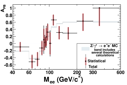
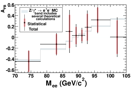
VII.4 Study of the $Z$-quark couplings using the $A_{FB}$ measurement

As seen in Sec. I, the vector and axial-vector nature of the interaction $\mbox{$\overline{p}p$}\rightarrow Z/\gamma^{*}\rightarrow e^{\rm+}e^{\rm-}$ renders the $A_{FB}$ measurement a direct probe of the relative strengths of the vector and axial-vector couplings between the quarks and the $Z$ boson. In this section, the effect of varying the $Z$-quark couplings on the forward-backward charge asymmetry of electron-positron pairs is investigated.

The $A_{FB}^{raw}$ measurement at detector level is compared to the following theoretical parameterization:

$$\mbox{$A_{FB}^{raw}$}(u_{V},u_{A},d_{V},d_{A})= \mbox{$A_{FB}^{raw}$}_{LO}(u_{V},u_{A},d_{V},d_{A})$$ (32)

$$-\mbox{$A_{FB}^{raw}$}_{LO}(SM)$$

$$+\mbox{$A_{FB}^{raw}$}_{\cal O(\alpha)}(SM),$$

where $A_{FB}^{raw}$_LO is the predicted $A_{FB}$ at the leading order and $A_{FB}^{raw}$_O(α) is the $A_{FB}$ calculated at the $\cal O(\alpha)$ electroweak corrections level with the ZGRAD generator described in Sec. VII.2. The quark couplings are changed at tree level assuming Standard Model couplings for the leptons. Both $A_{FB}^{raw}$_LO and $A_{FB}^{raw}$_O(α) are obtained after smearing the corresponding $A_{FB}^{phys}$with the parameterization presented in Sec. V.4. The parameterized $\mbox{$A_{FB}^{raw}$}(u_{V},u_{A},d_{V},d_{A})$, function of the $Z$-quark couplings, is compared to the measured $A_{FB}^{raw}$, and the best match is used to extract the coupling constants. Table 13 shows the coupling constants obtained after $\chi^{2}$ minimization, along with the corresponding statistical and systematic uncertainties. The $\chi^{2}$ divided by the number of degrees of freedom ($\chi^{2}$/DOF) equals 10.40/11.

	Coupling	Uncertainty
		Statistical	Systematic
uV	0.399	${}^{+0.152}_{-0.188}$	0.066
uA	0.441	${}^{+0.207}_{-0.173}$	0.067
dV	-0.226	${}^{+0.635}_{-0.290}$	0.090
dA	-0.016	${}^{+0.346}_{-0.536}$	0.091

Table 13: Vector and axial-vector quark couplings with statistical and systematic errors obtained from the fit to the $A_{FB}$ measurement at detector level.

The contribution from the different sources of systematic uncertainties on the quark coupling constants is given in Table 14, and the correlation matrix is shown in Table 15. For a given source of uncertainty, the systematic error on the coupling is calculated by repeating the fit using the measured $A_{FB}^{raw}$ shifted by its systematic uncertainty. The difference between the fitted coupling value obtained using the shifted $A_{FB}^{raw}$ and the nominal one is taken as the systematic uncertainty from that source. For the PDF uncertainty, we measured the couplings with four different parton distribution functions: MRST99, MRST2001, CTEQ6L and CTEQ5L (default). The uncertainty due to the PDF models is determined by the largest difference in the fitted coupling values with respect to the couplings obtained with CTEQ5L. The sign of the systematic uncertainty is defined in the same manner as in Table 10. Figure 25 displays the residuals compared to the SM $A_{FB}$ from the data (open markers) and from the fit (solid line) as a function of the invariant mass. The dashed curve corresponds to the residuals with the $u_{V}$ quark coupling shifted by 1$\sigma$.

Figure 25: Residuals compared to the SM $A_{FB}$ as a function of the invariant mass from the data (open marker) and from the fit (solid line). The dashed line represents the residuals with the $u_{V}$ coupling from the fit shifted by 1$\sigma$.

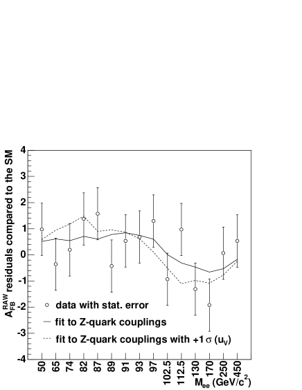
	En. scale	Resol.	material	bckgrd.	PDF
uV	-0.056	-0.023	-0.025	0.001	-0.001
uA	-0.013	-0.048	-0.009	-0.044	0.003
dV	-0.013	0.038	-0.076	-0.021	0.017
dA	-0.059	0.062	0.006	-0.025	-0.018

Table 14: Contribution of the different sources of systematic uncertainty on the quark coupling constants.

	uV	uA	dV	dA
uV	1.000	0.454	0.303	-0.037
uA	0.454	1.000	0.214	0.428
dV	0.303	0.214	1.000	0.548
dA	-0.037	0.428	0.548	1.000

Table 15: The correlation matrix of the statistical errors in the measurement of the up and down quark couplings.

The CDF sensitivity, with $\sim$72 $pb^{-1}$ of analyzed data, is limited, but the values of the couplings are consistent with the Standard Model. Figure 26 shows the contours at 68% and 90% confidence level for the $u$ (left) and $d$ (right) quark couplings to the $Z$ boson in the vector-, axial-vector basis. The closed markers correspond to the Standard Model predictions.

Figure 26: 68% and 90% confidence level contours for the $u$ (top) and $d$ (bottom) quark couplings to the $Z$ boson. The Standard Model predictions for these couplings are indicated by closed markers.

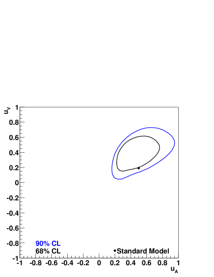
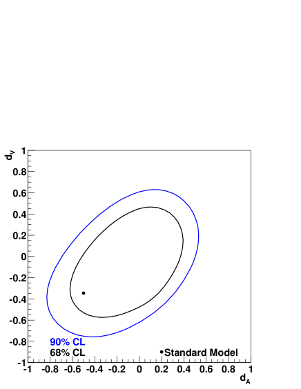
	This study	Exp. values Hagiwara et al. (2002)	SM prediction Hagiwara et al. (2002)
uL	0.419 ${}^{+0.131}_{-0.167}$	0.330 $\pm$ 0.016	0.3459 $\pm$ 0.0002
dL	-0.116 ${}^{+0.418}_{-0.352}$	-0.439 $\pm$ 0.011	-0.4291 $\pm$ 0.0002
uR	0.020 ${}^{+0.145}_{-0.150}$	-0.176 ${}^{+0.011}_{-0.006}$	-0.1550 $\pm$ 0.0001
dR	0.105 ${}^{+0.128}_{-0.315}$	-0.023 ${}^{+0.070}_{-0.047}$	0.0776

Table 16: Effective left- and right-handed coupling constants obtained from this study and compared to current experimental values and the Standard Model prediction from Hagiwara et al. (2002).

Table 16 summarizes the effective left- and right-handed coupling constants obtained from this study and compares them to the Standard Model prediction as well as the current experimental values of the effective couplings determined from ‘model independent’ fits to neutral-current data Hagiwara et al. (2002). As the present study is dominated by the statistical uncertainties, the sensitivity of these measurements will improve with higher integrated luminosities.

The $Z$-quark couplings returned by the fit are subsequently used to compute the $A_{FB}^{phys}$ which is shown for different invariant-mass bins in Table 17. The uncertainties in the resulting $A_{FB}^{phys}$ are the total (statistical and systematic) uncertainties from the fit of the $Z$ couplings. $A_{FB}^{phys}$ is then used to calculate the acceptance as discussed in Sec. V.5.

Bin	Mass Range	Fitted $A_{FB}^{phys}$
0	$40<M_{ee}<60$ GeV/c2	-0.170 $\pm$ 0.074
1	$60<M_{ee}<70$ GeV/c2	-0.355 $\pm$ 0.125
2	$70<M_{ee}<78$ GeV/c2	-0.373 $\pm$ 0.109
3	$78<M_{ee}<86$ GeV/c2	-0.183 $\pm$ 0.124
4	$86<M_{ee}<88$ GeV/c2	-0.044 $\pm$ 0.083
5	$88<M_{ee}<90$ GeV/c2	0.028 $\pm$ 0.053
6	$90<M_{ee}<92$ GeV/c2	0.088 $\pm$ 0.027
7	$92<M_{ee}<94$ GeV/c2	0.140 $\pm$ 0.039
8	$94<M_{ee}<100$ GeV/c2	0.223 $\pm$ 0.060
9	$100<M_{ee}<105$ GeV/c2	0.342 $\pm$ 0.087
10	$105<M_{ee}<120$ GeV/c2	0.429 $\pm$ 0.101
11	$120<M_{ee}<140$ GeV/c2	0.493 $\pm$ 0.135
12	$140<M_{ee}<200$ GeV/c2	0.506 $\pm$ 0.159
13	$200<M_{ee}<300$ GeV/c2	0.501 $\pm$ 0.171
14	$300<M_{ee}<600$ GeV/c2	0.498 $\pm$ 0.175

Table 17: Forward-Backward asymmetry calculated with the $Z$-quark coupling values returned by the fit. The uncertainties in $A_{FB}$ are based on the total (statistical and systematic) uncertainties on the $Z$ coupling values returned from the fit.

Assuming Standard Model $Z$-quark couplings, we can also determine the vector and axial-vector couplings between the electron and the $Z$-boson, using the same method. Table 18 shows the fitted electron coupling values along with statistical and systematic uncertainties. Combined LEP and SLD data LEP (2003) as well as the Standard Model prediction Hagiwara et al. (2002) are shown for comparison. The $\chi^{2}$/DOF of the fit equals to 13.14/13. For the present measurement, the uncertainties are dominated by the statistical uncertainties. The contributions of the different systematic uncertainties are given in Table 19. Note that the correlation coefficient between the vector and axial-vector couplings is 0.78.

	coupling	Stat.	Syst.	Total	SLD+LEP meas.	SM prediction
		err.	err.	err.
eV	-0.058	0.016	0.007	0.017	-0.03816 $\pm$0.00047	-0.0397 $\pm$0.0003
eA	-0.528	0.123	0.059	0.136	-0.50111 $\pm$0.00035	-0.5064 $\pm$0.0001

Table 18: Vector and axial-vector electron couplings with statistical and systematics uncertainties obtained from a fit to the $A_{FB}$ measurement. Combined LEP and SLD data LEP (2003) as well as the standard model prediction Hagiwara et al. (2002) are also given.

	En. scale	Resol.	material	bckgrd.	PDF
eV	-0.005	0.005	0.001	-0.001	0.001
eA	-0.002	0.055	0.006	-0.005	0.019

Table 19: Contribution of the different sources of systematic uncertainty on the electron coupling constants.

Finally a fit where the quark and electron couplings to the $Z$ boson are expressed as a function of $\sin^{2}\theta_{W}^{eff}$ gives:

$$\sin^{2}\theta_{W}^{eff}=0.2238\pm 0.0040(\rm stat)\pm 0.0030(\rm syst),$$ (33)

with a $\chi^{2}$/DOF equals to 12.50/14. The present CDF sensitivity on $\sin^{2}\theta_{W}^{eff}$ is provided by the $Z$-electron couplings and is expected to improve with higher statistics.

VII.5 $A_{FB}$ measurement assuming the fitted Standard Model couplings in the acceptance calculation

The total acceptance, $a^{\pm}_{cor}$, is calculated for each bin using the $A_{FB}^{phys}$ obtained from the $Z$ coupling fits (Table 17). The $A_{FB}$ measurements are corrected for acceptance, efficiency, resolution and bremsstrahlung using Eq. (15). The measured $A_{FB}$ and the prediction from PYTHIA using CTEQ5L parton distribution functions are listed in Table 20, and the measurements are compared with the Standard Model theoretical calculations (see Sec. VII.2) in Fig. 27. This technique, which is biased by the Standard Model input, is similar to the Run I analysis Affolder et al. (2001).

Mass Range	$<M_{ee}>$	Measured $A_{FB}$	PYTHIA $A_{FB}$
(GeV/$c^{2}$)	(GeV/$c^{2}$)
$40\leq\mbox{$M_{ee}$}<60$	48.2	-0.131 $\pm$ 0.108 $\pm$ 0.065	-0.214 $\pm$ 0.003
$60\leq\mbox{$M_{ee}$}<70$	64.9	-0.447 $\pm$ 0.095 $\pm$ 0.089	-0.420 $\pm$ 0.005
$70\leq\mbox{$M_{ee}$}<78$	74.3	-0.400 $\pm$ 0.072 $\pm$ 0.050	-0.410 $\pm$ 0.005
$78\leq\mbox{$M_{ee}$}<86$	83.0	-0.154 $\pm$ 0.043 $\pm$ 0.066	-0.214 $\pm$ 0.003
$86\leq\mbox{$M_{ee}$}<88$	87.1	0.002 $\pm$ 0.048 $\pm$ 0.041	-0.079 $\pm$ 0.004
$88\leq\mbox{$M_{ee}$}<90$	89.2	-0.015 $\pm$ 0.035 $\pm$ 0.021	-0.001 $\pm$ 0.002
$90\leq\mbox{$M_{ee}$}<92$	91.0	0.078 $\pm$ 0.031 $\pm$ 0.015	0.054 $\pm$ 0.001
$92\leq\mbox{$M_{ee}$}<94$	92.8	0.138 $\pm$ 0.033 $\pm$ 0.014	0.112 $\pm$ 0.002
$94\leq\mbox{$M_{ee}$}<100$	96.0	0.247 $\pm$ 0.034 $\pm$ 0.033	0.198 $\pm$ 0.003
$100\leq\mbox{$M_{ee}$}<105$	102.2	0.248 $\pm$ 0.099 $\pm$ 0.095	0.338 $\pm$ 0.006
$105\leq\mbox{$M_{ee}$}<120$	110.7	0.545 $\pm$ 0.091 $\pm$ 0.035	0.454 $\pm$ 0.006
$120\leq\mbox{$M_{ee}$}<140$	128.2	0.36${}^{+0.14}_{-0.15}$ $\pm$ 0.03	0.554 $\pm$ 0.002
$140\leq\mbox{$M_{ee}$}<200$	161.2	0.30${}^{+0.14}_{-0.15}$ $\pm$ 0.02	0.598 $\pm$ 0.002
$200\leq\mbox{$M_{ee}$}<300$	233.6	0.62${}^{+0.18}_{-0.24}$ $\pm$ 0.04	0.609 $\pm$ 0.004
$300\leq\mbox{$M_{ee}$}<600$	352.4	1.000${}^{+0.000}_{-0.64}$${}^{+0}_{-0.04}$	0.616 $\pm$ 0.007

Table 20: Experimental results for $A_{FB}$ along with statistical and systematic uncertainties and predictions from PYTHIA with CTEQ5L. The uncertainties on the PYTHIA predictions are MC statistical errors. The measured $A_{FB}$ values are corrected for acceptance, efficiency, resolution, and bremsstrahlung. The correction assumes the Standard Model and uses the $A_{FB}^{phys}$ derived from the fitted $Z$-quark coupling values. $<\mbox{$M_{ee}$}>$ is the cross section weighted average of the invariant mass in each bin.

Figure 27: Experimental results for $A_{FB}$ along with statistical and systematic uncertainties (crosses), and theoretical predictions based on the six calculations as described in Sec. VII.2 (bands). The measured $A_{FB}$ values are corrected for acceptance, efficiency, resolution, and bremsstrahlung. The correction assumes the Standard Model and uses the derived $A_{FB}^{phys}$ from the $Z$-quark coupling values. The bottom figure shows the $Z$ pole region in more detail.

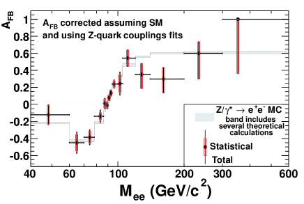
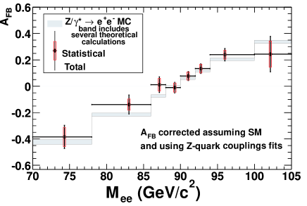
VIII Conclusions

We report a measurement of the forward-backward charge asymmetry ($A_{FB}$) of electron pairs resulting from the process $\mbox{$\overline{p}p$}\rightarrow Z/\gamma^{*}+X$ where $Z/\gamma^{*}\rightarrow e^{+}e^{-}$. The data are collected with the CDF II detector between March 2002 and January 2003, corresponding to about 72 pb^-1.

Comparisons have been made between the data and a simulated Standard Model prediction of the uncorrected $M_{ee}$ line shape, $\cos\theta^{*}$ distributions in three $M_{ee}$ regions, and $A_{FB}$ distribution. All comparisons give excellent agreement, with the uncorrected $A_{FB}$ distribution giving a $\chi^{2}$/DOF=15.7/15. The first principal result is a measurement of the corrected $A_{FB}$ in 15 $M_{ee}$ bins using an unfolding analysis that doesn’t assume a prior Standard Model $A_{FB}$ distribution. It has large uncertainties near the $Z$ pole because the $A_{FB}$ in those bins have large correlations. In the current dataset, there is no evidence of deviations from the Standard Model in the high $M_{ee}$ bins that might indicate non–Standard Model physics. The second principal result is a measurement of three sets of parameters: the $Z$-quark couplings, the $Z$-electron couplings, and $\sin^{2}\theta_{W}$. All three couplings measurements yield results consistent with the Standard Model. It may be possible to improve our understanding of the $Z$-quark couplings with a much larger dataset.