Statistical Analysis of Different Searches
Abstract
A combined statistical analysis of the experimental results of the LSND and KARMEN oscillation search is presented. LSND has evidence for neutrino oscillations that is not confirmed by the KARMEN experiment. This joint analysis is based on the final likelihood results for both data sets. A frequentist approach is applied to deduce confidence regions. At a combined confidence level of 36 %, there is no area of oscillation parameters compatible with both experiments. For the complementary confidence of %, there are two well defined regions of oscillation parameters (,) compatible with both experiments.
pacs:
14.60.St, 14.60.Pq, 06.20.Dk, 02.50.NgI Introduction
Currently, there are three neutrino anomalies interpreted as evidence for neutrino oscillations, namely the atmospheric atmo , the solar solar and the LSND LSNDfinal anomaly with three distinct squared neutrino mass differences. However, oscillations between the three Standard Model (SM) neutrinos are described by only two independent neutrino mass–squared differences, allowing only two of the above anomalies as being due to oscillations in a SM scenario extended by massive neutrinos. Before enlarging the neutrino sector by some additional, unknown sterile neutrinos, each of the experimental results has to be checked independently.
Over the last years, the controversial results of the two experiments LSND (Liquid Scintillator Neutrino Detector at LANSCE, Los Alamos, USA) and KARMEN (KArlsruhe Rutherford Medium Energy Neutrino experiment at ISIS, Rutherford, UK) both searching for neutrino oscillations in a short baseline regime, have led to intense discussions. The two experiments are similar as they use beams from the - decay at rest (DAR) chain + followed by e+ + + with energies up to 52 MeV. Furthermore, both experiments are looking for from oscillations according to the two–flavor oscillation probability 333In a comparison of different oscillation searches, one generally has to use a complete 3– or 4–dimensional description of neutrino masses and mixings, leading to the general oscillation probability. Since both experiments under investigation here have similar parameters and, most important, search for oscillations in the same appearance mode, the simplified formula holds for the purpose of the following analysis.
| (1) |
with the difference of the squared masses in eV2/c4, the flight length of the neutrino in meters and the neutrino energy in units of MeV. The detection reaction p ( , e+ ) n provides a spatially correlated delayed coincidence signature of a prompt e+ and a subsequent neutron capture signal.
This paper describes a combined statistical analysis of the final LSND and KARMEN 2 results. There are significant changes to the treatment of LSND data in the final LSND paper LSNDfinal . The present paper uses only the decay-at-rest (DAR) data, and leaves out the impact of the decay-in-flight (DIF) data. As shown later, the LSND data has a favored region in the 7 eV2/c4 region of as a consequence of this change. This is in contrast to the LSND result LSNDfinal which disfavors this solution at 90% C.L. because of the inclusion of the DIF flux. A motivation for this change is that a direct comparison of the two experiments is less model dependent if one considers the LSND DAR flux only, since KARMEN does not have a DIF neutrino flux present in its source.
The analysis is based on a frequentist approach following the suggestions of feldcous . For both experiments, the data are analysed with a maximum likelihood analysis followed by the extraction of confidence levels in a unfied approach. It is not the task nor the purpose of this analysis to treat the apparent disagreement between the two experiments. Rather, assuming no serious systematical error in either experiment or their interpretation with respect to oscillation, we apply a consistent statistical analysis to quantitatively establish their level of compatibility. The work follows an earlier analysis NJP based on intermediate data sets.
There are two separate questions investigated in this paper that relate to the LSND and KARMEN data. The first question is: at what level are the two data sets compatible with each other? This question addresses whether or not the two experiments force one to draw opposite conclusions from their respective data.
If one assumes that the data sets are compatible, the second question becomes: what are the most likely regions for the oscillation parameters? This method is somewhat analogous to treating the KARMEN data as coming from a ’near detector’ at 17 meters, and treating the LSND data as coming from a ’far detector’ at 30 meters. It ignores the question of systematic differences between the experiments, such as whether or not, for example, an unaccounted source of background neutrinos was present in the LSND data and not present in the KARMEN data.
The paper is organized as follows: After a short overview of the experimental setups of both experiments, section II describes the data analyses leading to likelihood functions of the oscillation parameters. Section III is devoted to the extraction of confidence regions for the individual experiments. In section IV, the experimental results are combined statistically, extracting levels of compatibility as well as oscillation parameters compatible with both experiments. We conclude with implications of this joint analysis, a comparison with other oscillation searches and an outlook to upcoming experimental tests of the favored oscillation parameters presented in this analysis.
I.1 The LSND experiment
The source of neutrinos for the LSND experiment was the interaction of the 798 MeV proton beam at the Los Alamos Neutron Science Center (LANSCE), in which a large number of pions, mostly are produced. The are mainly absorbed and only a small fraction decay to , which in turn are largely captured. Thus, the resulting neutrino source is dominantly due to + and e+ + + decays, most of which decay at rest (DAR). With a very small contamination of , a measurement of the reaction + p n + provides a sensitive way to search for oscillations. Such events are identified by detection of both the and the 2.2 MeV from the reaction p ( n, ) d. In addition, the flux from and decay-in-flight (DIF) is very small, which allows a search for oscillations via the measurement of electrons above the Michel electron endpoint from the reaction 12C ( , e- ) 12N.
The LSND experiment took data over six calendar years (1993-1998). During this period the LANSCE accelerator operated for 17 months, delivering 28 896 C of protons on the production target. The LSND detector bigpaper consisted of an approximately cylindrical tank 8.3 m long by 5.7 m in diameter. The center of the detector was located 30 m from the beam stop neutrino source. The tank was filled with liquid scintillator consisting of mineral oil and 0.031 g/l of b-PBD. This low scintillator concentration allowed the detection of both Čerenkov light and scintillation light. Photomultiplier time and pulse-height signals were used to reconstruct the track with an average RMS position resolution of cm and an energy resolution of % at the Michel endpoint of 52.8 MeV.
I.2 The KARMEN experiment
The KARMEN experiment used as neutrino source the pulsed spallation neutron source ISIS of the Rutherford Appleton Laboratory delivering 800 MeV protons. In contrast to the LANSCE source, the protons are extracted from the synchrotron as an intense but narrow double pulse, consisting of two parabolic pulses with a width of 100 ns separated by a peak-to-peak gap of 325 ns. The unique time structure of the ISIS proton pulses allowed a clear separation of neutrino-induced events from any beam unrelated background. The intrinsic contamination of the ISIS –beam is Bur96 .
The KARMEN detector drexlin was a rectangular high resolution liquid scintillation calorimeter, located at a mean distance of 17.7 m from the ISIS target at an angle of 100 degrees relative to the proton beam. The liquid scintillator was enclosed by a multilayer active veto system and a 7000 t steel shielding. The 65 m3 of liquid scintillator consisted of a mixture of paraffin oil (vol.), Pseudocumene (vol.) and 2 g/l scintillating additive 1-phenyl-3-mesityl-2-pyrazoline. The liquid scintillator volume was optically separated into 512 independent central modules. Gadolinium was implemented between the module walls for an efficient detection of thermal neutrons Gd ( n, ) with on average 3 ’s of energy MeV. The KARMEN detector as liquid scintillator calorimeter was optimized for high energy resolution of . Each event had energy, time and position information, as well as the number of addressed modules and their relative time differences.
The KARMEN 2 experiment took data from February 1997 to March 2001. During this time, protons equivalent to a total charge of 9425 Coulombs have been accumulated on the ISIS target. This corresponds to from the ISIS beam stop target.
II Data analysis and results as likelihood functions
For both experiments, a signal from oscillations consists of a spatially correlated delayed (e+,n) sequence from p ( , e+ ) n . Due to the different experimental techniques, the parameters to identify such sequences vary. Details of the LSND event reconstruction can be found in LSNDdet and bigpaper , the requirements for event sequences in KARMEN are described in K2paper .
In LSND, a (e+,n) sequence requires a prompt ’electron-like’ event with energy MeV followed by a low energy –event. The information about the delayed event is characterized via a likelihood ratio : If within one millisecond after the initial event another event is recorded at distance cm, the likelihood ratio in energy (PMT hits), time and distance of being a correlated p ( n, ) over an accidental coincidence is calculated, otherwise . Requiring a high likelihood ratio selects (e+,n) correlated events with low uncorrelated background, the so-called “gold-plated” events. However, to determine the oscillation parameters and in a likelihood analysis, an event sample with a much looser cut in is used, leading to higher efficiency for the oscillation channel, but naturally increasing the background. For the LSND sample analysed here, all the cuts described in LSNDfinal have been applied with two exceptions: The energy of the prompt event has been restricted to MeV instead of MeV and we applied a loose cut of instead of no -cut at all. The reason for these changes is twofold. First, the upper energy cut MeV excludes any significant influence of the channel on the much more sensitive channel. For any value of the oscillation parameter , the expected contribution from remains below 2 % of the signal. The second reason is a more technical one. Applying a unified frequentist approach to the likelihood function gained from the reduced data implies simulation and analysis of a large number of event samples analog to the experiment. Therefore, one is interested not to have too large samples containing mainly background events. With the cuts above, the original event sample is reduced by a factor of 5.5 to 1032 candidates, with an efficiency for at high reduced to 64.4 % of the original one (only 3.2 % of the expected events remain).
Figure 1 shows the event sample comprising 1032 beam-on events. Four variables are used to categorize the events:
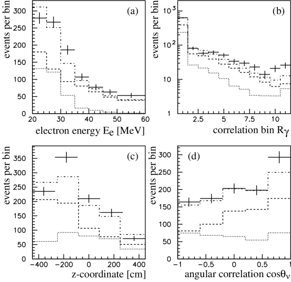
The energy of the primary electron , its spatial distribution along the detector axis 444The spatial coordinate along the detector axis can be easily referred to the neutrino flight path by adding the distance source–center of detector tank. and the angle between the direction of the incident neutrino and the reconstructed electron path. The fourth variable is the likelihood ratio for a (e+,n) coincidence. The binning of this distribution with the upper edge of bin number representing a value has been chosen for practical reasons. Note that the spectra in Figure 1 are projections of a 4-dim space of correlated parameters for each event. Superimposed to the data are shown the beam-unrelated and beam-related background contributions amounting to a total number of events. The expected background contributions are broken down in Table 1, for further details we refer to LSNDfinal .
| Contribution | Signal or Background Source | Process | Expected Number of Events |
|---|---|---|---|
| 1 | 11350115 | ||
| 2 | BUB | 635.026.2 | |
| 3 | DAR | 312.218.5 | |
| 4 | DIF | 7.4 | |
| 5 | DIF | 3.9 | |
| 6 | DAR ( DAR) | 12.4 | |
| 7 | 22730 | ||
| 8 | DIF and decay | 1.0 |
Formally, each beam-on event of the candidates is assigned a probability equal to a sum of probabilities from the backgrounds plus oscillations. The vector describes herein the spectral parameters of each event , . It then remains to add the with expected fractional contributions and take the product over all the beam-on events. The likelihood is thus
| (2) |
where
| (3) |
Additionally, two normalization requirements must hold:
| (4) |
and
| (5) |
for each contribution, . Together, these requirements ensure that every observed beam-on event has a probability of occurrence equal to 1.
To allow for the fact that the backgrounds are known to some limited accuracy only, the background is varied by calculating the above likelihood at each point in the (,) plane many times, varying over the expected for each background. For each background configuration, the is weighted with a Gaussian factor for each background that is off its central value. The background variations are performed in a simplified manner, i.e. the beam-unrelated background (BUB) varies independently and all the beam-related backgrounds (BRBs) are locked together. Finally, the likelihood can be expressed as
| (6) |
where the represents, schematically, the background variation described above. Integrating over different background contributions eventually reduces the free parameters of the likelihood procedure from to the 2 free parameters of real interest within this analysis, the oscillation parameters:
| (7) |
Figure 2 shows the logarithm of the event–based likelihood
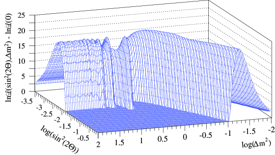
function, , for the 1032 events investigated. The maximum is reached at a parameter combination (=0.85, =0.055 eV2/c4) corresponding to a total oscillation signal of . The difference to the no–oscillation hypothesis as expressed in logarithmic likelihood units is
| (8) |
underlining the significance of the additional signal among the event sample. Note that the extracted oscillation events scale with the efficiency of the applied cuts and are in good agreement with the best fit result stated in LSNDfinal .
KARMEN 2 collected data from February 1997 through March 2001 corresponding to 9425 C accumulated proton charge on the ISIS target. A spatial coincidence between the initial e+ and the neutron capture of 1.3 m3 was required. Applying all cuts to the data K2paper , 15 (e+,n) candidate sequences were finally reduced. Figure 3 shows the remaining sequences in the appropriate energy, time and spatial windows.
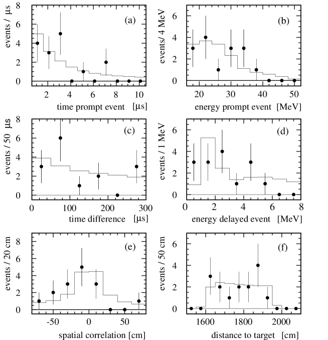
The background components are also given with their distributions. All components except the intrinsic contamination are measured online in different time and energy windows (see Table 2).
| Process | Expectation | Determination |
|---|---|---|
| Cosmic induced background | measured in diff. time window | |
| Charged current coincidences | measured in diff. energy, time windows | |
| –induced random coincidences | measured in diff. time window | |
| source contamination | MC–simulation | |
| Total background | ||
The extracted number of sequences is in excellent agreement with the background expectation, consistent with no oscillation signal. To also include the detailed spectral information of each individual event, a maximum likelihood method is applied.
Analogously to the LSND likelihood function, we can define the combined likelihood for the KARMEN sample as
| (9) |
where
| (10) |
with and , the oscillation signal as well as 4 background contributions. For KARMEN 2, the vector has, of course, a different definition, namely describing the energy and time relative to beam-on-target of the prompt event, the energy of the delayed event as well as the time difference and spatial correlation of the prompt and delayed event. Again, normalizations (4) and (5) with the appropriate event parameters have to hold. Differing from the likelihood definition in the LSND analysis, for KARMEN with its very small background, all background components are combined into one contribution, therefore reducing the above sum (10) to only the oscillation signal and the total background, . Furthermore, the weight for the background variation, defined in (6) as a Gaussian factor, is taken as Gamma function, reflecting a continuous variation in a Poisson statistics K2paper .
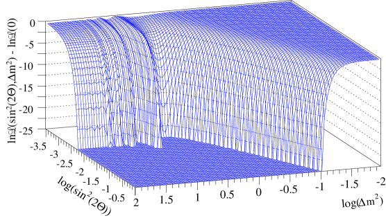
Figure 4 shows the logarithm of the likelihood as a function of the oscillation parameters (,). The maximum is reached near the physical boundary , i.e. the no–oscillation case. The sharp drop in towards larger values of demonstrates that there is no indication for an oscillation signal.
A typical approach to deduce confidence regions from likelihood functions would consist of defining the contour of an area of given confidence by cutting the likelihood function at the corresponding value below the maximum. For a Gaussian shaped likelihood function of two uncorrelated free parameters, the corresponding values would be
| (11) |
for confidence, respectively Lyons . However, this method leads to correct coverage only in the Gaussian case. As can be seen from Figures 2 and 4 the likelihood functions have distinct features: An oscillatory behavior as a function of the free parameters, the maximum at the physical boundary (for KARMEN), or numerous side maxima with comparable likelihood values (for LSND). In addition, the parameter space in (,) is, in principle, not limited, its metric in terms of prior probability density not unequivocally defined.
III Individual confidence regions
The method we apply in the following is based on a unified frequentist approach suggested by feldcous which eliminates the bias that occurs when one decides, after analysing the data, between using a confidence interval (having a positive signal) or an upper confidence limit (having a result compatible with the background). When first presented, it was argued that the suggested ordering principle near the physical boundary should be modified Giunti ,Byron , or that a Bayesian approach to the extracted likelihood function would be more appropriate Dagos . However, many experimental results have been analysed since using the unified approach CWCL , also being described as a standard procedure by Pdg2000 .
The basic idea of the unified frequentist approach is to create a large number of event samples in perfect analogy to an experiment. These samples are created by Monte Carlo using the full event information for the likelihood procedure. For an oscillation hypothesis with given parameters (,)H, a large sample of Monte Carlo simulations of so-called toy experiments is created. These simulations are based on the detailed knowledge of all experimental resolution functions and the spectral information on the individual background contributions. In addition, they comprise the expected experimental signal for the given oscillation hypothesis 555For each individual sample, the number of background events as well as the number of signal events vary according to the error of the expectation values.. For each likelihood function of the analysed samples, the estimator is calculated by comparing each sample’s likelihood maximum with the value for the given input parameters (,)H. The hypothesis is then accepted at a confidence , if the estimator of the experimental likelihood function is contained within the smallest % of the simulated estimator distribution. Since, in principle, the estimator distribution itself is a function of the oscillation parameters, a complete statistical analysis consists of a scan of the entire parameter space (,) to extract the according region of confidence.
III.1 KARMEN
To deduce confidence regions from the KARMEN 2 likelihood function, the parameter space (,) has been scanned extracting the estimator distribution for 8000 different oscillation hypotheses, including the no–oscillation scenario. From these distributions, each containing the information of about 4000 simulated and analysed samples, regions of different confidence levels can be calculated.
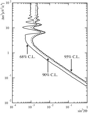
Figure 5 shows the regions of the oscillation parameters (,) for confidence levels of 68 %, 90 % and 95 %. Parameter combinations to the right contain the complementary confidence. The contours of the confidence areas are often referred to as exclusion curves of a given confidence. For values eV2/c4, the contours cut at oscillation amplitudes of (68 % C.L.), (90% C.L.) and (95% C.L.).
The KARMEN 2 sensitivity, defined as expectation value for the upper limit of a given confidence interval under the assumption of no oscillations, is again obtained by simulations: for 68 % C.L. (90% C.L., 95% C.L.), respectively. The error on the contour lines is given by the statistical error of the estimator’s cut value and therefore depends on the amount of simulated samples per hypothesis and the degree of confidence under consideration. For example, determining from a distribution of 1000 simulated samples relies on the upper 10 % tail or the highest 100 values. We derive the error on from the spread of the cut value taking the upper samples. For KARMEN 2, the typical relative error on is in the range of %.
III.2 LSND
For the LSND likelihood function, the method to deduce the confidence regions is identical to the one described in section III.1 for KARMEN 2. Technically, however, there are differences due to the large amount of computing time. This arises from the fact that the event samples are much larger (about 1000 events, depending on the oscillation parameters, instead of about 15) and the integration over different background contributions according to equation (6) is performed in as much as 255 discrete steps of different backgrounds BUB and BRB.
| DAR+DIF | 68 % | 90 % | 95 % | |
|---|---|---|---|---|
| 0.0 | 0.0 | |||
| 33.5+0.2 | ||||
| 67.1+0.4 | ||||
| 134.2+0.8 | ||||
Therefore, we restricted the hypotheses tested from a fine grid for KARMEN 2 to some grid points representing the typical variation of expected oscillation events. For a fixed oscillation parameter eV2/c4, 4 oscillation scenarios were simulated with 1000 individual samples each (see Table 3).
As verified by earlier calculations NJP and the KARMEN 2 analysis, the main variation of for a given confidence in the parameter space (,) follows the variation of the signal strength, i.e. the number of oscillation events among the event sample. We therefore extrapolated the values of in Table 3 linearly with and adopted, at each grid point (,) with its expected number of oscillation events , the estimator value . Having constructed the estimator cut distribution this way, the last step is analogous to that used for KARMEN 2, i.e. to cut the LSND likelihood function with the given values below the maximum and draw the contour lines. Figure 6 shows the contour lines of areas containing 68 %, 90 % and 95 % confidence.
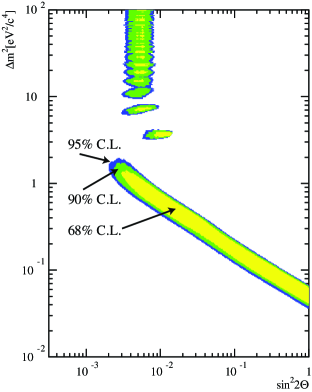
Although parameter combinations with eV2/c4 are part of the 90% C.L. area, they are scarcely included in the more stringent interval of 68 % confidence, demonstrating the lower likelihood values for such oscillation scenarios.
It is useful to compare the extracted confidence regions with the favored regions given in LSNDfinal where the likelihood function had been calculated based on a larger event sample (5697 events with MeV and no –cut). In addition, a simplified extraction of confidence regions according to equation (11) had been applied 666In fact, due in part to the larger statistical sample, in LSNDfinal the results of such a simplified procedure were shown to be similar to the results obtained from an approximation to a full unified frequentist approach..
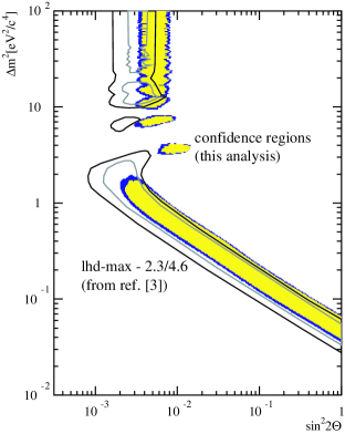
Figure 7 shows, that for lower values of , there is only a slight shift to larger oscillation amplitudes of the new analysis. A large overlap of the 90% C.L. area with the region according to demonstrates the good statistical agreement of the analyses of both event samples. For higher values of , the differences are more pronounced. Compared to the older analysis, the confidence region is not only shifted considerably to larger amplitudes, but the likelihood values themselves are larger relative to the likelihood maximum which results in a larger area of 90% C.L.. These effects can be understood by the upper energy cut MeV applied in the actual analysis. Restricting the analysis mainly to the oscillation channel favors also large values of whereas a signal from , derived in LSNDfinal to be much smaller, but detectable mainly at higher energies, decreases the likelihood for such solutions as well as the absolute strength or oscillation amplitude.
Finally, we note the importance to derive values of leading to correct coverage of confidence regions. These values differ considerably from the simplified Gaussian approach of a constant of 2.3 units. In an earlier analysis of the LSND data NJP , the typical estimator cut values were on the basis of about 3000 events. Now, with even smaller event samples, the values of further increase to . This dependance of is also underlined by the typical values for the much smaller KARMEN 2 sample size, where ranges from 3 to 5.
IV Compatibility Analysis
Having analysed both experiments’ likelihood functions with the same consistent method, we can now use this method and its results to deduce quantitative statements on the question of statistical compatibility of both experimental results and, in the case of such compatibility, on the common parameter combinations (,).
IV.1 Level of compatibility
One of the most misleading but nevertheless very frequently used interpretation of the LSND and KARMEN results is to take the LSND region left over from the KARMEN exclusion curve as area of (,) favored by both experiments. Such an interpretation, though appealingly straight forward, completely ignores the information of both likelihood functions and reduces them to two discrete levels of a specific confidence . To be able to correctly combine the two experimental results and extract the combined confidence regions, we have to use the original estimator distributions for KARMEN and for LSND. In a first step, the level of statistical compatibility of the two experimental outcomes has to be quantified. In the second step, the parameters favored by both experiments will be deduced.
In the following analysis, an experiment or event, in logical terms of frequency or probability of occurence, means repeating both, the KARMEN and the LSND experiment. Compatibility is then achieved if there are at least some oscillation parameters being the element of both the repeated KARMEN-like and LSND-like experiment’s confidence region.
We make the well justified assumption that the two experiments LSND and KARMEN are independent. Then, a two dimensional estimator distribution can be constructed for each hypothesis from the individual distributions of KARMEN and of LSND by an inverse projection. For each hypothesis, the pair of experimental values is checked to be part of the ’inner’ % of the simulated 2–dimensional estimator distribution. There are different methods of ordering these 2–dimensional distributions all leading to very similar results NJP . In the following, we require each experimental value and to be contained in the corresponding 1–dimensional interval of confidence. This selection criterion is equivalent to selecting a rectangle of frequency of the 2–dim estimator distribution. The resulting confidence is . Since we do not weight the experiments, we define , so that for a combined confidence of e.g. 81 %, we demand and .
At a level of , no parameter combination (,) fulfills the requirement any more. This corresponds to the fact that, at the level of combined confidence
| (12) |
the two experiments are completely incompatible. Coming back to our definition of probability of occurence, in 64 % of repetitions of double experiments, a KARMEN 2 plus an LSND experiment with their typical parameters and statistics, the outcome would consist of statistically compatible results with a specified set of oscillation parameters (, ).
IV.2 Common oscillation parameters
In the following, we analyse the preferred regions of oscillation parameters in the case of compatibility defined in the section before. If two experiments are independent producing two likelihood functions as result of the event analysis, the recipe for a combined analysis is straight forward. The likelihoods can be multiplied, i.e. in our case the logarithms of the likelihood functions are added. The absolute values of the likelihood functions are somewhat arbitrary. A recommended presentation of is to normalize the individual functions and to a point in (,) where they are equally sensitive to a potential signal dagos2 . In our case of the oscillation search this corresponds to values of . Therefore we define the combined likelihood function
| (13) | |||||
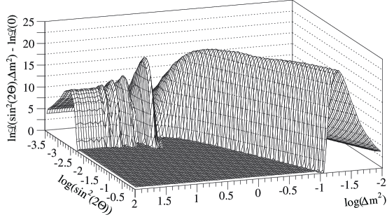
Figure 8 shows the combined function with a maximum of (1,0.05)21.5 on a long flat ’ridge’ of low values. The positive signal of LSND dominates the combined likelihood. However, the maximum in comparison to the no–oscillation value is reduced (see Equ. 8) as well as the shape at higher values of is significantly modified due to the KARMEN 2 likelihood function.
To determine the confidence regions in (,), again we apply the unified approach, i.e. we create the estimator distribution K+L for various hypotheses (,)H and compare the experiment’s value KARMEN2+LSND with the cut value for a given confidence. To get the estimator, a simulated event sample now consists of a KARMEN 2-like and an LSND-like MC sample each analysed with the appropriate likelihood definitions. Then both likelihood functions are added following equation (13) and the estimator is calculated.
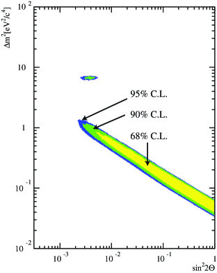
The typical cut values for a confidence of % are slightly higher than the individual LSND ones, ranging from 3.5 to 5.5. Figure 9 shows the confidence regions of the oscillation parameters for the combined likelihood analysis. The total confidence of a parameter region is hereby reduced by the fraction of incompatibility of the two experiments, so
| (14) |
which results in e.g. % total confidence for the parameter combinations within the area denoted as 90% C.L. area in Figure 9.
The combination of both experiments’ results with this consistent frequentist approach demonstrates that solutions with eV2/c4 are excluded. There remain essentially two solutions in the parameter space of oscillations, one at eV2/c4 and the area with eV2/c4. The latter one, though graphically rather large in Figure 9 corresponds to just one solution in the ’phase space’ of oscillations: Any signal from oscillation has rather low energy, the evolution of the oscillation probability (equ. 1) being just at the beginning of the oscillation length. With an oscillation parameter eV2/c4, and a typical lower energy of MeV from decay at rest, the first maximum of oscillations of into would be at a distance
| (15) |
from the neutrino source. For such oscillation parameters, the negative result of KARMEN 2 compared to the excess of LSND mainly reflects the different detector distances m versus m from the source. This is one way to reconcile the results of the two experiments.
To summarize, at a joint confidence level of %, the two experiments are either incompatible or lead to just one single oscillation solution at eV2/c4. The remaining 20 % confidence separate into an enlargement of the parameter region of low values and into a second oscillation solution at eV2/c4.
V Conclusion
We have analysed both the KARMEN 2 and the LSND final data with a maximum likelihood method using a similar event–based likelihood function. The likelihood functions as functions of the free parameters and demonstrate the different outcomes of the experiments, namely a clear, statistically significant excess of in LSND versus no indication of an oscillation signal in KARMEN 2. To deduce regions of correct coverage, we applied a unified frequentist approach to both likelihood analyses individually. The results underline the feasibility of as well as the necessity for such an approach.
A quantitative joint statistical analysis has been performed leading to a level of 36 % incompatibility of the experimental outcomes, corresponding to individual confidence levels of 60 %. For the cases of statistical compatibility, the common parameter regions have been identified on the basis of the unified frequentist approach applied to the combined likelihood function of KARMEN 2 and LSND. The derived confidence regions in (,) clearly differ from an often applied but incorrect graphical overlap of the confidence regions of the individual experiments. There are two oscillation scenarios with either eV2/c4 or eV2/c4 compatible with both experiments.
We performed a joint statistical analysis incorporating some of the systematic uncertainties of the experiments, such as neutrino flux uncertainty, accuracy of known cross sections and resolution functions of both experiments.
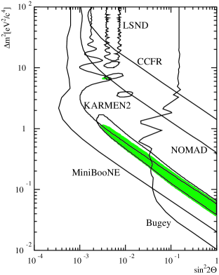
Further –unknown– systematic uncertainties might become evident only by performing new experiments to confirm or discard the results described here. Figure 10 shows the intended sensitivity of a new experiment, MiniBooNE at Fermilab BooNE , which is under construction and will independently crosscheck the LSND evidence.
In addition, we did not incorporate the results of other experiments on the oscillation parameters investigated. As shown in Figure 10, the deduced favored region in (,) is partly overlaped by 90% C.L. exclusion curves of other experiments. In particular, the recent NOMAD result NOMAD clearly reduces the overall likelihood for the eV2/c4 solution. A complete analysis should include these results on the basis of the same statistical method, i.e. a consistent frequentist analysis. This implies, however, the detailed knowledge of experimental data and resolution functions of these experiments not accessible to us. Furthermore, the exclusion curve from the Bugey experiment is based on the disappearance search . Combining this experiment correctly with the appearance results of or in terms of mixing angles would therefore also require a full three– or four–dimensional mixing scheme with theoretical models including sterile neutrinos bilenky ; Hirsch ; Ioann ; Ma ; Lorenz ; strumia or CPT violation barenb and would become model-dependent.
VI Acknowledgements
We would like to thank the members of both collaborations for the encouragement and help to make this final joint analysis possible. In particular, we acknowledge the support of and many discussions with W.C. Louis concerning the LSND as well as G. Drexlin concerning the KARMEN experiment. Without the openness and trust to analyse both data sets in detail, such an analysis wouldn’t have been feasible. K.E. also wants to thank the Alexander von Humboldt foundation for financial support during visits to the Los Alamos National Laboratory. Clarifying discussions with Kai Zuber on the principles of combining experiments with contradictory central statements were very helpful.
References
-
(1)
S. Fukuda et al. (Super-Kamiokande), Phys. Rev. Lett. 85, 3999 (2000);
M. Ambrosio et al. (MACRO), Phys. Lett B 517, 59 (2001). -
(2)
B. T. Cleveland et al. (Homestake), Astrophys. J. 496, 505 (1998);
W. Hampel et al. (Gallex), Phys. Lett. B 447, 127 (1999);
J. N. Abdurashitov et al. (SAGE), Phys. Rev. C 60, 055801 (1999);
S. Fukuda et al. (Super-Kamiokande), Phys. Rev. Lett. 86, 5651 (2001); 86, 5656 (2001);
M. Altmann et al. (GNO), Phys. Lett. B 490, 16 (2000);
Q. R. Achmad et al. (SNO), Phys. Rev. Lett. 87, 071301 (2001). - (3) A. Aguilar et al., Phys. Rev. D 64, 112007 (2001).
- (4) G. J. Feldman and R. D. Cousins, Phys. Rev. D 57, 3873 (1998).
- (5) K. Eitel, New Jour. Phys. 2, 1.1 (2000).
- (6) C. Athanassopoulos et al., Phys. Rev. C 54, 2685 (1996).
-
(7)
R. L. Burman, M. E. Potter, and E. S. Smith,
Nucl. Instrum. Methods A 291, 621 (1990);
R. L. Burman, A. C. Dodd, and P. Plischke, Nucl. Instrum. Methods A 368, 416 (1996). -
(8)
G. Drexlin et al., Nucl. Instrum. Methods A 289, 490 (1990);
G. Drexlin, Progr. Part. Nucl. Phys 40, 193 (1998). - (9) C. Athanassopoulos et al., Nucl. Instrum. Methods A 388, 149 (1997).
- (10) B. Armbruster et al., Phys. Rev. D (submitted), Los Alamos e-print xxx.lanl.gov hep-ex/0203021.
-
(11)
For reviews, see L. Lyons, Statistics for nuclear and particle physicists
(Cambridge University Press, 1986);
W. T. Eadie et al., Statistical Methods in Experimental Physics (North Holland, Amsterdam and London, 1971). - (12) C. Giunti, Phys. Rev. D 59, 053001 (1999).
- (13) B. P. Roe, M. B. Woodroofe, Phys. Rev. D 60, 053009 (1999).
- (14) G. D’Agostini, Bayesian Reasoning in High-Energy Physics and Applications (CERN Report CERN-99-03).
- (15) F. James et al., Proceedings of the Workshop on Confidence Limits, CERN, Geneva, 2000 (CERN Report CERN-2000-005).
- (16) D. E. Groom et al., Eur. Phys. J. C 15, 1 (2000).
- (17) G. D’Agostini, Los Alamos e-print xxx.lanl.gov hep-ex/0002055.
- (18) B. Achkar et al., Nucl. Phys. B 434, 503 (1995).
- (19) A. Romosan et al., Phys. Rev. Lett. 78, 2912 (1997).
- (20) V. Valuev, Proceedings of the International Europhysics Conference on HEP 2001.
- (21) A. O. Bazarko, Nucl. Phys. B (Proc. Suppl.) 91, 210 (2001).
- (22) S. M. Bilenky et al., Progr. Part. Nucl. Phys 43, 1 (1999).
- (23) M. Hirsch and J. W. F. Valle, Phys. Lett. B 495, 121 (2000).
- (24) A. Ioannisian and J. W. F. Valle, Phys. Rev. D 63, 073002 (2001).
- (25) E. Ma and G. Rajasekaran, Phys. Rev. D 64, 117303 (2001).
- (26) A. Perez-Lorenzana and C. A. de S. Pires, Phys. Lett. B 522, 297 (2001).
- (27) A. Strumia, Los Alamos e-print xxx.lanl.gov hep-ph/0201134.
- (28) G. Barenboim et al., Phys. Rev. D 65, 053001 (2002).