I Introduction

Inflationary universe model[1] is the most favorite scenario which can explain the large scale homogeneity and isotropy of the Universe. One of the main questions concerning the inflation is whether the occurrence of inflation is generic or not.

There are lots of investigations on this problem in the homogeneous model universes. For Friedmann-Robertson-Walker universe with an inflaton[2, 3], the occurrence of inflation is generic except the closed universe case. In the view point of cosmological no-hair conjecture, Wald[4] showed that initially expanding anisotropic Bianchi type universes with a positive cosmological constant except the type IX approach de Sitter universe. In theses cases, inflation is not completely generic because the positive spatial curvature can prevent inflation.

It is obvious that the most appealing feature of the inflationary cosmologies is smoothing out the initial inhomogeneities of the universe. Thus, we should clarify the generality of inflation in the initially inhomogeneous universe. The effect of inhomogeneities on the inflation is studied by numerical simulations [5, 6] . In Ref.[5], it is shown that the homogeneity over a few initial horizon is needed in order to inflate the universe and other works support it.

There are two aspects of the inhomogeneities. One is the inhomogeneities of the inflaton, the other is the one in the metric. In general these are coupled. In this paper we study how the inhomogeneities of the spatial geometry affect the occurrence of inflation by the use of the long wavelength approximation, which reduces the Einstein equations to several sets of ordinary differential equations.

By the use of the long wavelength approximation method we can construct approximate solutions of Einstein equations which describe an inhomogeneous universe on scales larger than the local Hubble radius. Belinski, Khalatnikov and Lifshitz[7] studied the general behaviors of the universe in the neighborhood of initial singularity by this approximation, and Tomita[8] focused attentions on the evolutions of inhomogeneities of the early universe in this framework.

The long wavelength approximation assumes that the spatial derivative of a metric is smaller than the time derivative. The spatial curvature which consists of the spatial derivative of the second order is neglected in the lowest order of this approximation and it is taken into account perturbatively by the series expansion in the higher order. This approximation is called the gradient expansion method for the Einstein equations. For the higher order solutions, Comer, Deruelle, Langlois et al[9] developed an iteration scheme of Einstein equations and Salopek, Stewart et al[10] developed one of the Hamilton-Jacobi equation for general relativity.

Recently, using the gradient expansion method, the generality of inflation is discussed by Deruelle and Goldwirth[11], and Nambu and Taruya[12]. As shown by the investigations of the homogeneous models[3, 4], the positive spatial curvature plays an essential role; if the positive curvature dominates over the vacuum energy, which drives inflation, the universe never enter the inflationary era and recollapse to the singularity. In the marginal solution between inflationary and recollapsing solution, the spatial curvature becomes as large as the vacuum energy. For desired inflation to explain the homogeneity of the universe, large vacuum energy is necessary. Then we should take account of non-small spatial curvature to clarify the condition for the occurrence of inflation. Readers would suspect that the gradient expansion method is not suitable for investigation of the generality of inflation because the spatial curvature is assumed to be a small quantity.

In this paper, we improve the gradient expansion scheme so that the non-small constant spatial curvature can be tractable in the lowest order. By this improved gradient expansion scheme, we study how the inhomogeneities of the spatial curvature affect the occurrence of inflation in the closed universe. The word ‘closed universe’ does not mean the universe with spatial surface of closed topology in this paper. We investigate the time evolution of the spatial region with non-small positive spatial curvature.

For the first step to investigate the effect of the inhomogeneities of the spatial curvature for the onset of inflation we consider the model in which the cosmological constant gives rise to inflation instead of the scalar field and a radiation fluid fills the universe.

This paper is organized as follows. In Sec.2, we explain the improved gradient expansion method in order to construct the inhomogeneous closed universe. And we derive the basic equations in the first order approximation. In Sec.3, we specify the basic equations for our simple model and show numerical results for our aim. Sec.4 is devoted to conclusion and discussions.

II Gradient Expansion from Closed Friedmann Universe

In this section, we review the usual gradient expansion method briefly and modify it so that non-vanishing spatial curvature is included in the lowest order.

A Brief Review

We start from a brief review of the usual gradient expansion method.

Take a synchronous reference frame where the line element is

$$ds^{2} = -dt^{2}+\gamma_{ij}(t,x^{k})dx^{i}dx^{j}.$$

Throughout this paper Latin letters will denote spatial indices and Greek letters spacetime indices. The matter is taken to be a perfect fluid characterized by energy-momentum tensor

$\displaystyle T_{\mu\nu}=(\rho+p)u_{\mu}u_{\nu}+pg_{\mu\nu},$

where $p,\rho$ and $u_{\mu}$ are pressure, energy density and four velocity, respectively. We assume the equation of state of the fluid is $p/{\rho}\equiv{\Gamma}-1$, where $\Gamma$ is a constant. The Einstein equations with a cosmological constant $\Lambda$ are

$${}^{3}\!R_{i}^{j}+\frac{1}{2\sqrt{\gamma}}\frac{\partial}{\partial t}(\sqrt{\gamma}K_{i}^{j}) = \frac{2\dot{K}+K_{l}^{m}K_{m}^{l}-4\Lambda}{4(2-3\Gamma-2\Gamma u_{l}u^{l})}[2\Gamma u_{i}u^{j}+\delta_{i}^{j}(2-\Gamma)]+\Lambda\delta_{i}^{j},$$ (1)

$$\kappa\rho = \frac{2\dot{K}+K_{l}^{m}K_{m}^{l}-4\Lambda}{2(2-3\Gamma-2\Gamma u_{l}u^{l})},$$ (2)

$$\kappa\Gamma\rho u_{i} = -\frac{1}{2\sqrt{1+u_{l}u^{l}}}(K_{i;j}^{j}-K_{,i}),$$ (3)

where ${}^{3}\!R_{i}^{j}$ is the Ricci tensor associated with $\gamma_{ij}$, $K_{ij}\equiv\dot{\gamma}_{ij}$ is the extrinsic curvature, $\gamma\equiv\det\gamma_{ij}$, a dot denotes the derivative with respect to $t$, a semicolon denotes the covariant derivative with respect to $\gamma_{ij}$ and $\kappa\equiv 8\pi G$.

We consider the situation in which all spatial gradients are much smaller than time derivatives and assume that the spatial metric is expanded as

$$\gamma_{ij}(t,x)=\stackrel{{\scriptstyle(0)}}{{\gamma}}_{ij}(t,x)+\stackrel{{\scriptstyle(1)}}{{\gamma}}_{ij}(t,x)+\cdots=\sum_{p}\stackrel{{\scriptstyle(p)}}{{\gamma}}_{ij}(t,x).$$ (4)

Here the lowest term $\stackrel{{\scriptstyle(0)}}{{\gamma}}_{ij}$ in Eq.(4) is assumed in the quasi isotropic form

$$\stackrel{{\scriptstyle(0)}}{{\gamma}}_{ij}(t,x)=a^{2}(t)h_{ij}(x),$$ (5)

where $a(t)$ is the scale factor in the lowest order which depends on only $t$ and $h_{ij}(x)$ is an arbitrary function of only spatial variables. The next-order term $\stackrel{{\scriptstyle(1)}}{{\gamma}}_{ij}$ is constructed by the symmetric tensors of the second order in the spatial gradients of $h_{ij}$ in the form

$$\stackrel{{\scriptstyle(1)}}{{\gamma}}_{ij}(t,x)=a^{2}(t)\left[f_{1}(t)R_{ij}(h)+g_{1}(t)R(h)h_{ij}\right],$$ (6)

where $R_{ij}(h)$ is the Ricci tensor associated with $h_{kl}(x)$, $R(h)\equiv h^{ij}R_{ij}(h)$, and $f_{1}(t)$ and $g_{1}(t)$ are functions of time. The subsequent general terms $\stackrel{{\scriptstyle(p)}}{{\gamma}}_{ij}$ in Eq.(4) are spatial tensors which are of order $2p$ in the spatial gradients of $h_{ij}(x)$ with time dependent coefficients. Since the spatial inhomogeneities of the spacetime is generated by $h_{ij}(x)$, then we call it ‘seed metric’.

Substituting Eq.(5) into Eqs.(1)-(3) and neglecting the spatial derivatives we get the lowest (zeroth) order solution

$$a(t)=\left[\sinh\left(\frac{3\Gamma}{2}H_{0}t\right)\right]^{\frac{2}{3\Gamma}},$$ (7)

$$\stackrel{{\scriptstyle(0)}}{{\rho}}=\frac{3H_{0}^{2}}{\kappa\sinh^{2}(\frac{3\Gamma}{2}H_{0}t)},$$ (8)

$$\stackrel{{\scriptstyle(0)}}{{u}}_{i}=0,$$ (9)

where $H_{0}\equiv\sqrt{\Lambda/3}$. The evolution of scale factor at zeroth order is the same as the one of flat Friedmann-Robertson-Walker universe. So, we call the solution described by Eqs.(7)-(9) “locally flat Friedmann solution”.

At next (first) order, substituting the spatial metric $\gamma_{ij}=\stackrel{{\scriptstyle(0)}}{{\gamma}}_{ij}+\stackrel{{\scriptstyle(1)}}{{\gamma}}_{ij}$ given by Eqs.(5) and (6) into Eq.(1) and taking the spatial derivative terms of the seed metric, we get ordinary differential equations for the functions of time $f_{1}(t)$ and $g_{1}(t)$(see ref.[9]). Similarly, we can calculate the higher order solutions iteratively. The locally flat Friedmann universe, Eqs.(7)-(9), is used as a starting point to solve Eq.(1) in the expansion scheme, thus we call this scheme the gradient expansion from the flat Friedmann universe (GEFF). In GEFF, the spatial curvature is treated perturbatively as a small quantity in the series expansion.

B Improved method

In this subsection we improve GEFF such that we can treat non-vanishing three curvature which is discarded at lowest order. We show that when the seed metric has maximally symmetry, the closed or open Friedmann solution is derived by summing up all terms in GEFF. After that we extend the method such that the inhomogeneities around the closed or open Friedmann universe are tractable.

First, we consider a seed metric in the maxmally symmetric form with non-vanishing curvature:

$$h_{ij}(x)=h^{\pm}_{ij}(x),$$

where the Ricci curvature associated with the metric is

$$R_{ij}(h^{\pm})=\pm 2h^{\pm}_{ij}.$$

Since all spatial tensors of rank two derived from $h^{\pm}_{ij}$ are proportional to $h^{\pm}_{ij}$ itself, then time dependent part in Eq.(4) is factorized in the form

$$\gamma_{ij}(t,x) = a^{2}(t)\left[h^{\pm}_{ij}+f_{1}(t)R_{ij}(h^{\pm})+g_{1}(t)R(h^{\pm})h^{\pm}_{ij}+f_{2}(t)R(h^{\pm})R_{ij}(h^{\pm})+\cdots\right]$$ (10)

$$= a_{\pm}^{2}(t)h^{\pm}_{ij}(x),$$ (11)

where

$$a_{\pm}^{2}(t)\equiv a^{2}(t)\Big{[}1\pm\{2f_{1}(t)+6g_{1}(t)\}+\{12f_{2}(t)+\cdots\}+\cdots\Big{]}.$$ (12)

Substituting Eq.(11) into Eqs.(1)-(2) we obtain the equation which $a_{\pm}$ must satisfy:

$$\frac{\ddot{a}_{\pm}}{a_{\pm}}-\frac{2-3\Gamma}{2}\left(\frac{\dot{a}_{\pm}}{a_{\pm}}\right)^{2}\mp\frac{2-3\Gamma}{2a_{\pm}^{2}} = \frac{\Gamma}{2}\Lambda,$$ (13)

$$\left(\frac{\dot{a}_{\pm}}{a_{\pm}}\right)^{2}\pm\frac{1}{a_{\pm}^{2}} = \frac{1}{3}(\kappa\rho+\Lambda).$$ (14)

These are nothing but the equations for the closed or open Friedmann universe. Of course, the universe described by the solution satisfying these equations is far from the flat Friedmann universe but no more than the homogeneous universe.

Next, we consider the inhomogeneities of the spatial curvature. Here we think a simple case where the inhomogeneities are expressed by one spatial function. We take the seed metric to be conformal to the metric of constant curvature,

$$h_{ij}(x)=\Omega^{2}(x)h^{\pm}_{ij}(x),$$ (15)

where $\Omega(x)$ is an arbitrary spatial function.

In this case, the Ricci and scalar curvature are given by

$$R_{ij}(h_{kl}(x)) = \pm 2h^{\pm}_{ij}(x)-\frac{\nabla_{i}\nabla_{j}\Omega}{\Omega}+2\frac{\nabla_{i}\Omega\nabla_{j}\Omega}{\Omega^{2}}-\frac{\nabla_{l}\nabla^{l}\Omega}{\Omega}h^{\pm}_{ij}$$ (16)

$$R(h_{kl}(x)) = \frac{1}{\Omega^{2}}\{\pm 6-4\frac{\nabla_{l}\nabla^{l}\Omega}{\Omega}+2\frac{\nabla_{l}\Omega\nabla^{l}\Omega}{\Omega^{2}}\},$$ (17)

where $\nabla_{i}$ is the covariant derivative with respect to $h^{\pm}_{ij}$. The spatial metric, therefore, in the expansion form Eq.(4) becomes

$$\gamma_{ij}(t,x) = a^{2}(t)\left[h_{ij}+f_{1}(t)R_{ij}(h)+g_{1}(t)R(h)h_{ij}+f_{2}(t)R(h)R_{ij}(h)+\cdots\right]$$ (18)

$$= a^{2}(t)\Bigg{[}\left\{\Omega^{2}\pm(2f_{1}(t)+6g_{1}(t))+\Omega^{-2}(12f_{2}(t)+\cdots)+\cdots\right\}h^{\pm}_{ij}$$ (24)

$$\qquad-\left\{(f_{1}(t)+4g_{1}(t))+\Omega^{-2}(\pm 14f_{2}(t)+\cdots)+\cdots\right\}\frac{\nabla_{l}\nabla^{l}\Omega}{\Omega}h^{\pm}_{ij}$$

$$\qquad+\{2g_{1}(t)+\Omega^{-2}(\pm 4f_{2}(t)+\cdots)+\cdots\}\frac{\nabla_{l}\Omega\nabla^{l}\Omega}{\Omega^{2}}h^{\pm}_{ij}$$

$$\qquad-\{f_{1}(t)+\Omega^{-2}(\pm 6f_{2}(t)+\cdots)+\cdots\}\frac{\nabla_{i}\nabla_{j}\Omega}{\Omega}$$

$$\qquad+\{2f_{1}(t)+\Omega^{-2}(\pm 12f_{2}(t)+\cdots)+\cdots\}\frac{\nabla_{i}\Omega\nabla_{j}\Omega}{\Omega^{2}}$$

$$\qquad+\left\{\Omega^{-2}(4f_{2}(t)+\cdots)+\cdots\right\}\left(\frac{\nabla_{l}\nabla^{l}\Omega}{\Omega}\right)^{2}h^{\pm}_{ij}+\cdots\Bigg{]}$$

Here we consider the situation that the spatial derivative of $\Omega$ is small. From Eq.(17), it means that the derivative of spatial curvature is smaller than the value of curvature itself.

Introducing

$$a^{2}_{\pm}(t,x)\equiv a^{2}(t)\left[\Omega^{2}(x)\pm\{2f_{1}(t)+6g_{1}(t)\}+\Omega^{-2}(x)\{12f_{2}(t)+\cdots\}+\cdots\right],$$ (25)

we rewrite Eq.(24) as

$$\gamma_{ij}(t,x) = a_{\pm}^{2}(t,\Omega)\left[h^{\pm}_{ij}+\sum_{A}F_{(2)}^{A}(t,\Omega)(\nabla^{(2)}\Omega)^{A}_{ij}+\sum_{A}F_{(4)}^{A}(t,\Omega)(\nabla^{(4)}\Omega)^{A}_{ij}+\cdots\right.$$ (27)

$$\left.\qquad+\sum_{A}F_{(2p)}^{A}(t,\Omega)(\nabla^{(2p)}\Omega)^{A}_{ij}+\cdots\right].$$

Here the notation $(\nabla^{(2p)}\Omega)^{A}_{ij}$ denotes symbolically symmetric spatial tensors which contain $2p$ spatial gradients of $\Omega(t,x)$, where the suffix $A$ distinguishes the tensor belonging to the same class, and $F_{(2p)}^{A}(t,\Omega)$ is a function of $t$ and $\Omega(x)$ which is determined by the Einstein equations later. This is nothing but a re-summation of the usual gradient expansion. We restrict ourselves to consider the situation which the series expansion Eq.(27) converges.

Substituting Eq.(27) into Eqs.(1) and (2) and neglecting the spatial gradients of $\Omega$ we obtain Eqs.(13) and (14) again for $a_{\pm}(t,x)$ for the zeroth order solution

$$\stackrel{{\scriptstyle(0)}}{{\gamma}}_{ij}{\hskip-9.95845pt}^{\pm}(t,x) = a_{\pm}^{2}(t,\Omega(x))h^{\pm}_{ij}(x).$$ (28)

In contrast to Eq.(12), the behavior of $a_{\pm}(t,x)$, defined by Eq.(25), depends on $\Omega(x)$. The solution of Eqs.(13) and (14) is the same form of closed (open) Friedmann universe. The new expansion scheme Eq.(27) is based on the local closed (open) Friedmann universe, so we call it “the gradient expansion from a locally closed (open) Friedmann universe” (GECF (GEOF)).

Next, we consider the parts of the second order in spatial gradients of $\Omega(x)$ in Eq.(27). The tensors $(\nabla^{(2)}\Omega)^{A}_{ij}$ are four types and $\stackrel{{\scriptstyle(1)}}{{\gamma}}_{ij}{\hskip-9.95845pt}^{\pm}(t,x)$ is in the form

$$\stackrel{{\scriptstyle(1)}}{{\gamma}}_{ij}{\hskip-9.95845pt}^{\pm}(t,x) = a_{\pm}^{2}(t,x)\left[\frac{1}{3}F(t,\Omega)\frac{\nabla_{l}\nabla^{l}\Omega}{\Omega}h^{\pm}_{ij}+\bar{F}(t,\Omega)\overline{\frac{\nabla_{i}\nabla_{j}\Omega}{\Omega}}\right.$$ (30)

$$\qquad\left.+\frac{1}{3}G(t,\Omega)\frac{\nabla_{l}\Omega\nabla^{l}\Omega}{\Omega^{2}}h^{\pm}_{ij}+\bar{G}(t,\Omega)\overline{\frac{\nabla_{i}\Omega\nabla_{j}\Omega}{\Omega^{2}}}\right],$$

where $\overline{\nabla_{i}\nabla_{j}\Omega/\Omega}$ and $\overline{\nabla_{i}\Omega\nabla_{j}\Omega/\Omega^{2}}$ are defined by

$$\overline{\frac{\nabla_{i}\nabla_{j}\Omega}{\Omega}}\equiv\frac{\nabla_{i}\nabla_{j}\Omega}{\Omega}-\frac{1}{3}\frac{\nabla_{l}\nabla^{l}\Omega}{\Omega}h^{\pm}_{ij},\qquad\overline{\frac{\nabla_{i}\Omega\nabla_{j}\Omega}{\Omega^{2}}}\equiv\frac{\nabla_{i}\Omega\nabla_{j}\Omega}{\Omega^{2}}-\frac{1}{3}\frac{\nabla_{l}\Omega\nabla^{l}\Omega}{\Omega^{2}}h^{\pm}_{ij}.$$

From Eq.(3) we obtain

$$u_{i} = \frac{(2-3\Gamma)\left[2\left(\dot{a}_{\pm}^{\prime}/{a_{\pm}}-{\dot{a}_{\pm}a_{\pm}^{\prime}}/{a_{\pm}^{2}}\right)\Omega-\dot{\bar{F}}\right]}{2\Gamma\left[3\ddot{a}_{\pm}/a_{\pm}-\Lambda\right]}\frac{\nabla_{i}\Omega}{\Omega},$$ (31)

where the prime denotes the differentiation with respect to $\Omega$.

Substituting $\gamma_{ij}=\stackrel{{\scriptstyle(0)}}{{\gamma}}_{ij}{\hskip-9.95845pt}^{\pm}+\stackrel{{\scriptstyle(1)}}{{\gamma}}_{ij}{\hskip-9.95845pt}^{\pm}$ and $u_{i}$ given by Eqs.(28), (30) and (31) into Eq.(1), and comparing the coefficients of the second order derivative terms of $\Omega$, we obtain

$$\ddot{F}+3\Gamma\frac{\dot{a}_{\pm}}{a_{\pm}}\dot{F}=-\frac{(2-3\Gamma)}{a_{\pm}^{2}}\left[\pm F-\bar{F}+2\frac{a_{\pm}^{\prime}\Omega}{a_{\pm}}\right],$$ (32)

$$\ddot{\bar{F}}+3\frac{\dot{a}_{\pm}}{a_{\pm}}\dot{\bar{F}}=\frac{2}{a_{\pm}^{2}}\left[\frac{a_{\pm}^{\prime}\Omega}{a_{\pm}}+2(\pm\bar{F}-\bar{F})\right],$$ (33)

$$\ddot{\tilde{G}}+3\Gamma\frac{\dot{a}_{\pm}}{a_{\pm}}\dot{\tilde{G}}=-\frac{(4-3\Gamma)(2-3\Gamma)}{2\Gamma a_{\pm}\left(3\ddot{a}_{\pm}-\Lambda a_{\pm}\right)}\left[\dot{\bar{F}}-2\left(\frac{\dot{a}_{\pm}^{\prime}}{a_{\pm}}-\frac{\dot{a}_{\pm}a_{\pm}^{\prime}}{a_{\pm}^{2}}\right)\Omega\right]^{2}$$ (34)

$$\qquad\qquad\qquad-\frac{(2-3\Gamma)}{a_{\pm}^{2}}\left[\pm G+\bar{F}-{\bar{F}}^{\prime}\Omega\pm 2{\bar{F}}^{2}-{\bar{F}}^{2}+\Omega^{2}\left(2\frac{a_{\pm}^{\prime\prime}}{a_{\pm}}-\frac{a_{\pm}^{\prime 2}}{a_{\pm}^{2}}\right)\right],$$ (35)

$$\ddot{\hat{G}}+3\frac{\dot{a}_{\pm}}{a_{\pm}}\dot{\hat{G}}=\frac{(2-3\Gamma)}{\Gamma a_{\pm}\left(3\ddot{a}_{\pm}-\Lambda a_{\pm}\right)}\left[\dot{\bar{F}}-2\left(\frac{\dot{a}_{\pm}^{\prime}}{a_{\pm}}-\frac{\dot{a}_{\pm}a_{\pm}^{\prime}}{a_{\pm}^{2}}\right)\Omega\right]^{2}$$ (36)

$$\qquad\qquad\qquad+\frac{2}{a_{\pm}^{2}}\left[\pm 2\bar{G}+2\bar{F}-2{\bar{F}}^{\prime}\Omega-(\pm 2+\frac{1}{2})\bar{F}^{2}-2\left(\frac{a_{\pm}^{\prime}\Omega}{a_{\pm}}\right)^{2}+\frac{a_{\pm}^{\prime\prime}\Omega^{2}}{a_{\pm}}\right],$$ (37)

where we put $\tilde{G}\equiv G+{\bar{F}}^{2}$ and $\hat{G}\equiv\bar{G}-\frac{1}{2}{\bar{F}}^{2}$ for simplicity of the equation form. To solve Eq.(32)- Eq.(37), we need to know the time evolution of $\bar{F}^{\prime}$. Differentiating Eq.(33) we find that $\bar{F}^{\prime}$ must satisfy the equation

$$\ddot{\bar{F}}^{\prime}+3\frac{\dot{a}_{\pm}}{a_{\pm}}\dot{\bar{F}}^{\prime} = \frac{2}{a_{\pm}^{2}}\left[\frac{a^{\prime}_{\pm}}{a_{\pm}}+\frac{a^{\prime\prime}_{\pm}\Omega}{a_{\pm}}-3\frac{{a^{\prime}_{\pm}}^{2}\Omega}{a_{\pm}^{2}}-4\frac{a^{\prime}_{\pm}}{a_{\pm}}(\pm\bar{F}-\bar{F})+2(\pm\bar{F}^{\prime}-\bar{F}^{\prime})\right]$$ (39)

$$-3\dot{\bar{F}}\left[\frac{\dot{a}^{\prime}_{\pm}a_{\pm}-\dot{a}_{\pm}a^{\prime}_{\pm}}{a^{2}_{\pm}}\right].$$

III Inflation in the inhomogeneous universe with a positive curvature

In this section, we consider how the inhomogeneities of spatial curvature affect on the occurrence of inflation. For this purpose we think a simple model, in which the inflation is driven by a cosmological constant $\Lambda$. We construct the inhomogeneous universe by the gradient expansion from the closed Friedmann universe which is introduced in the previous section. The matter is taken to be a radiation fluid with $\Gamma=4/3$ for simplicity.

We get the lowest order solution of Eqs.(13) and (14) for the system in the form

$$a_{+}^{2}(t,\Omega(x))\equiv\frac{1}{2H_{0}^{2}}\left[2H_{0}^{2}\Omega^{2}\sinh(2H_{0}t)+1-\cosh(2H_{0}t)\right],$$ (1)

$$\stackrel{{\scriptstyle(0)}}{{\rho}}=\frac{3H_{0}^{2}\Omega^{4}}{\kappa a_{+}^{4}}.$$ (2)

Here we see the behavior of the locally closed Friedmann solution Eq.(1). The solution has an early phase during which the local scale factor behaves as $a_{+}\propto t^{1/2}$. After the period the behavior of local scale factor depends on the local value of $\Omega(x)$. The local scale factor $a_{+}(t,x)$ with $\Omega(x)>\Omega_{cr}$ approaches de Sitter solution and $a_{+}(t,x)$ with $\Omega(x)<\Omega_{cr}$ recollapses to the singularity, where $\Omega_{cr}\equiv\sqrt{1/(2H^{2}_{0})}$. The local scale factor $a_{+}(t,x)$ with the critical value of $\Omega=\Omega_{cr}$ approaches a static solution

$$a_{+}^{2}=\frac{3}{2\Lambda},\quad\stackrel{{\scriptstyle(0)}}{{\rho}}=\frac{\Lambda}{\kappa}.$$ (3)

In the early stage $t<<H_{0}^{-1}$, the local scale factor is proportional to $\Omega(x)t^{1/2}$ then the spatial curvature ${}^{3}\!R$ is proportional to $1/(\Omega^{2}t)$. The fate of local scale factor is determined by the value of ${}^{3}\!R(t,x)t$ in the lowest order. The condition for the occurrence of inflation is

$$\frac{1}{\Omega^{2}}<\frac{1}{\Omega_{cr}^{2}}.$$ (4)

In other words, it is

$${}^{3}\!R_{init}<{}^{3}\!R_{cr}(t)\equiv\frac{3}{\Omega_{cr}^{2}}\frac{1}{H_{0}t},$$ (5)

where ${}^{3}\!R_{init}$ is the spatial curvature in the early phase $t<<H_{0}^{-1}$.

Next, we consider the first order corrections which are proportional to the second order of spatial gradients of $\Omega(x)$ in the form

$$\stackrel{{\scriptstyle(1)}}{{\gamma}}_{ij}{\hskip-9.95845pt}^{+}(t,x) = a_{+}^{2}(t,\Omega(x))\Bigg{[}\frac{1}{3}F(t,\Omega)\frac{\nabla_{l}\nabla^{l}\Omega}{\Omega}h^{+}_{ij}+\bar{F}(t,\Omega)\overline{\frac{\nabla_{i}\nabla_{j}\Omega}{\Omega}}$$ (7)

$$\qquad\qquad\qquad+\frac{1}{3}G(t,\Omega)\frac{\nabla_{l}\Omega\nabla^{l}\Omega}{\Omega^{2}}h^{+}_{ij}+\bar{G}(t,\Omega)\overline{\frac{\nabla_{i}\Omega\nabla_{j}\Omega}{\Omega^{2}}}\Bigg{]}.$$

From Eqs.(32)-(39), the equations for $F,\bar{F},G$ and $\bar{G}$ reduce to

$$\ddot{F}+4\left(\frac{\dot{a}_{+}}{a_{+}}\right)\dot{F} = \frac{2}{a_{+}^{2}}\left[F-\bar{F}+\frac{2\Omega^{2}\sinh(2H_{0}t)}{a_{+}^{2}}\right],$$ (8)

$$\ddot{\tilde{G}}+4\left(\frac{\dot{a}_{+}}{a_{+}}\right)\dot{\tilde{G}} = \frac{2}{a_{+}^{2}}\left[\tilde{G}+\bar{F}-\bar{F}^{\prime}\Omega+\frac{\Omega^{2}\sinh(2H_{0}t)}{a_{+}^{2}}\left(2-\frac{3\Omega^{2}\sinh(2H_{0}t)}{a_{+}^{2}}\right)\right],$$ (9)

$$\ddot{\bar{F}}+3\left(\frac{\dot{a}_{+}}{a_{+}}\right)\dot{\bar{F}} = \frac{2}{a_{+}^{2}}\left[\frac{\Omega^{2}\sinh(2H_{0}t)}{a_{+}^{2}}\right],$$ (10)

$$\ddot{\hat{G}}+3\left(\frac{\dot{a}_{+}}{a_{+}}\right)\dot{\hat{G}} = \frac{2}{a_{+}^{2}}\left[2\hat{G}+2\bar{F}-2{\bar{F}}^{\prime}\Omega-\frac{3\bar{F}^{2}}{2}+\frac{\Omega^{2}\sinh(2H_{0}t)}{a_{+}^{2}}\left(1-\frac{3\Omega^{2}\sinh(2H_{0}t)}{a_{+}^{2}}\right)\right]$$ (12)

$$+\frac{1}{2H_{0}^{4}\Omega^{4}a_{+}^{6}}\left[2\Omega^{2}(\cosh(2H_{0}t)-1)-H_{0}a_{+}^{4}\dot{\bar{F}}\right]^{2}.$$

For $\bar{F}^{\prime}$ we get

$$\ddot{\bar{F}}^{\prime}+3\frac{\dot{a}_{+}}{a_{+}}\dot{\bar{F}}^{\prime} = \frac{4\Omega\sinh(2H_{0}t)}{a_{+}^{4}}\left[1-\frac{2\Omega^{2}\sinh(2H_{0}t)}{a_{+}^{2}}\right]-3\dot{\bar{F}}\frac{\Omega}{H_{0}a_{+}^{4}}(\cosh(2H_{0}t)-1).$$ (13)

We solve Eqs.(8)-(13) by numerical integration. These coupled ordinary differential equations have growing and decaying solutions. In the course of time, since the growing mode dominates the solution we concentrate on the growing solution. Then we choose initial conditions for $F,\bar{F},\bar{F}^{\prime},\tilde{G},\hat{G}$ in the form

$$F=\bar{F}=\bar{F}^{\prime}=\tilde{G}=\hat{G}=0.$$ (14)

The growing mode is generated by the source terms in the right hand side of Eqs.(8)-(13). For the regularity, asymptotic behaviors of these variables should be

$$F=\frac{1}{\Omega^{2}H_{0}}t,\quad\bar{F}=\frac{2}{3\Omega^{2}H_{0}}t,\quad\bar{F}^{\prime}=-\frac{4}{3\Omega^{3}H_{0}}t,\quad\tilde{G}=-\frac{1}{2\Omega^{2}H_{0}}t,\quad\hat{G}=-\frac{4}{3\Omega^{2}H_{0}}t.$$ (15)

Time evolution of $F$ and $\tilde{G}$ is shown in Figs.1 and 2. In the case of $\Omega>\Omega_{cr}$, $F$ and $G$ grow for a while and become constant as the universe expands exponentially. And in the case of $\Omega<\Omega_{cr}$, they grow and diverge and the approximation breaks down.

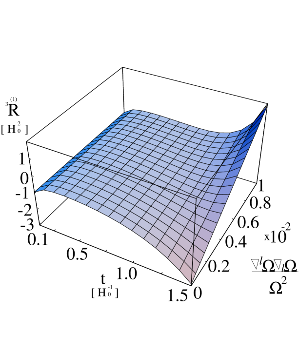
We demonstrate a time evolution of the spatial scalar curvature given by Eq.(B13) (see Fig.3). When we fix initial time, there are infinite number of combinations of parameters $(\Omega,\nabla_{l}\nabla^{l}\Omega/\Omega,\nabla_{l}\Omega\nabla_{l}\Omega/\Omega^{2})$ which give the same value of ${}^{3}\!R$. Time evolution of ${}^{3}\!R$ depends on the parameters. Fixing $\Omega$, we vary $\nabla_{l}\Omega\nabla_{l}\Omega/\Omega^{2}$ and $\nabla_{l}\nabla^{l}\Omega/\Omega$ keeping ${}^{3}\!R$ constant. When $\Omega$ is fixed, since the evolution of ${}^{3}\!\stackrel{{\scriptstyle(0)}}{{R}}$ depends only on $\Omega$, the time evolution of ${}^{3}\!R$ depends on $\nabla_{l}\Omega\nabla_{l}\Omega/\Omega^{2}$. We see from Fig.3 that when $\nabla_{l}\Omega\nabla_{l}\Omega/\Omega^{2}$ is large ${}^{3}\!R$ grows rapidly.

By the use of the trace part of the corrections, we define an effective local scale factor which includes up to the first order by

$$a_{\mbox{\sl eff}}(t,x) \equiv \left[\det\Big{[}\stackrel{{\scriptstyle(0)}}{{\gamma}}_{ij}{\hskip-9.95845pt}^{+}+\stackrel{{\scriptstyle(1)}}{{\gamma}}_{ij}{\hskip-9.95845pt}^{+}\Big{]}\right]^{1/6}$$ (16)

$$= a_{+}(t,\Omega)\left[1+\frac{1}{6}F(t,\Omega)\frac{\nabla_{l}\nabla^{l}\Omega}{\Omega}+\frac{1}{6}\tilde{G}(t,\Omega)\frac{\nabla_{l}\Omega\nabla^{l}\Omega}{\Omega^{2}}\right].$$ (17)

The effective local scale factor $a_{\mbox{\sl eff}}(t,x)$ describes how the universe expands at the point $x$.

We can follow the evolution of the effective local scale factor $a_{\mbox{\sl eff}}(t,x)$ by the evolution of $F(t,\Omega)$ and $G(t,\Omega)$. As is already seen, at lowest order the behavior of local scale factor $a_{+}(t,\Omega)$ is determined by the value of $\Omega(x)$. On the other hand, the spatial derivatives of $\Omega$ affect the time evolution of $a_{\mbox{\sl eff}}(t,x)$ at first order. It means that the effective local scale factor evolves under the influence of the local value of $\Omega$ and the value of it in the neighborhood. If a point in the three dimensional parameter space $(\Omega,\nabla_{l}\nabla^{l}\Omega/\Omega,\nabla_{l}\Omega\nabla_{l}\Omega/\Omega^{2})$ is specified we know the time evolution of the effective local scale factor $a_{\mbox{\sl eff}}(t,x)$.

The effective local expansion rate and acceleration rate are given by

$$\frac{\dot{a}_{\mbox{\sl eff}}}{a_{\mbox{\sl eff}}} = \frac{\dot{a}_{+}}{a_{+}}+\frac{1}{6}\left[\dot{F}(t,\Omega)\frac{\nabla_{l}\nabla^{l}\Omega}{\Omega}+\dot{\tilde{G}}(t,\Omega)\frac{\nabla_{l}\Omega\nabla^{l}\Omega}{\Omega^{2}}\right],$$

$$\frac{\ddot{a}_{\mbox{\sl eff}}}{a_{\mbox{\sl eff}}} = \frac{\ddot{a}_{+}}{a_{+}}+\frac{1}{6}\left[\ddot{F}(t,\Omega)+2\frac{\dot{a}_{+}}{a_{+}}\dot{F}(t,\Omega)\right]\frac{\nabla_{l}\nabla^{l}\Omega}{\Omega}+\frac{1}{6}\left[\ddot{\tilde{G}}(t,\Omega)+2\frac{\dot{a}_{+}}{a_{+}}\dot{\tilde{G}}(t,\Omega)\right]\frac{\nabla_{l}\Omega\nabla^{l}\Omega}{\Omega^{2}}.$$

When the correction terms which contain the second order derivatives grow to be as large as the lowest order term, the expansion scheme breaks down. Since the first order terms in Eq.(27) contain all of the second order spatial derivatives then when $(\dot{a}_{+}/a_{+})^{2}>{}^{3}\!\stackrel{{\scriptstyle(0)}}{{R}}$, GECF reduces to GEFF. We, thus, assume the approximation is valid while

$$\left|\frac{\det(\stackrel{{\scriptstyle(0)}}{{\gamma}}_{ij}{\hskip-9.95845pt}^{+}+\stackrel{{\scriptstyle(1)}}{{\gamma}}_{ij}{\hskip-9.95845pt}^{+})-\det\stackrel{{\scriptstyle(0)}}{{\gamma}}_{ij}{\hskip-9.95845pt}^{+}}{\det\stackrel{{\scriptstyle(0)}}{{\gamma}}_{ij}{\hskip-9.95845pt}^{+}}\right| < 0.5,$$ (18)

$$\left|\frac{{}^{3}\!\!\stackrel{{\scriptstyle(1)}}{{R}}}{\max\{(\dot{a}_{+}/a_{+})^{2},{}^{3}\!\!\stackrel{{\scriptstyle(0)}}{{R}}\}}\right| < 0.5.$$ (19)

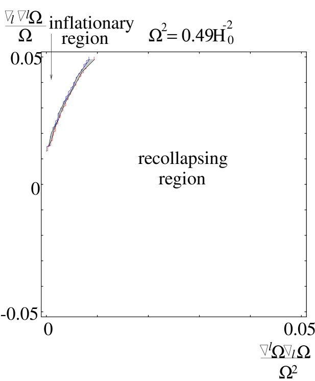
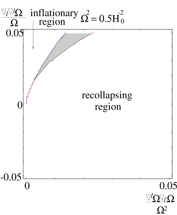
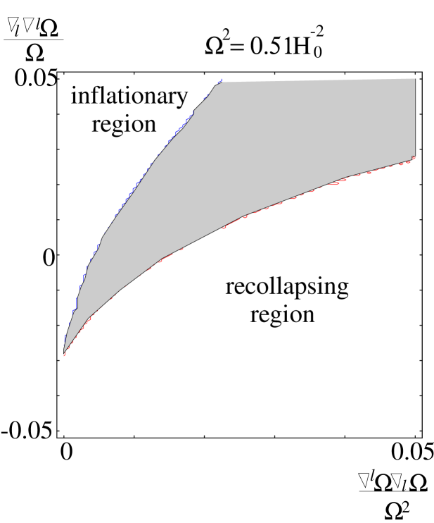
We divide the three dimensional parameter space $(\Omega,\nabla_{l}\nabla^{l}\Omega/\Omega,\nabla_{l}\Omega\nabla_{l}\Omega/\Omega^{2})$ into two regions: inflationary region and recollapsing region (see Figs.4 - 6). The effective local scale factor with the parameters in the inflationary region enters the accelerating expansion phase: $\dot{a}_{\mbox{\sl eff}}/a_{\mbox{\sl eff}}>0$ and $\ddot{a}_{\mbox{\sl eff}}/a_{\mbox{\sl eff}}>0$. On the other hand, the effective local scale factor with the parameters in the recollapsing region enters recollapsing phase: $\dot{a}_{\mbox{\sl eff}}/a_{\mbox{\sl eff}}<0$ and $\ddot{a}_{\mbox{\sl eff}}/a_{\mbox{\sl eff}}<0$. Between these two regions, there emerges a fuzzy region where error becomes large and Eq.(18) or Eq.(19) does not hold before the effective local scale factor enters the inflationary or recollapsing phase.

IV Conclusion and Discussions

We studied how the inhomogeneities of spatial curvature affect the occurrence of inflation in the inhomogeneous universe which is constructed by the gradient expansion from the locally closed Friedmann universe, in which the inhomogeneities are described by a function $\Omega(x)$ and its spatial gradients. For the first step, we considered a simple model universe with a cosmological constant and radiation fluid.

In this paper, we expanded the spatial metric up to the second order spatial derivatives $\nabla_{i}\nabla_{j}\Omega/\Omega$ and $\nabla_{i}\Omega\nabla_{j}\Omega/\Omega^{2}$. We solved the ordinary differential equations for the coefficient functions of these derivative terms numerically and evolved the inhomogeneous spatial metric[13]. We assumed that the inhomogeneities were generated by one function $\Omega(x)$ but the universe needed not to have any symmetries.

How the inhomogeneities described by $\nabla_{l}\nabla^{l}\Omega/\Omega$ and $\nabla_{l}\Omega\nabla^{l}\Omega/\Omega^{2}$ affect the onset of inflation is shown in Figs.4 - 6. The term $\nabla_{l}\Omega\nabla^{l}\Omega/\Omega^{2}$ tends to prevent inflation and positive (negative) $\nabla_{l}\nabla^{l}\Omega/\Omega$ helps the universe to inflate (collapse). This is related to the fact that the spatial curvature grows rapidly when $\nabla_{l}\Omega\nabla^{l}\Omega/\Omega^{2}$ is large.

From Figs.4 - 6, we get the criterion for the occurrence of inflation in the vicinity of $\Omega/\Omega_{cr}-1=\nabla_{l}\nabla^{l}\Omega/\Omega=\nabla_{l}\Omega\nabla^{l}\Omega/\Omega^{2}=0$ in a simple time independent form:

$$\frac{1}{\Omega^{2}}\left[1+\alpha\left\{-\frac{\nabla_{l}\nabla^{l}\Omega}{\Omega}+\beta\frac{\nabla_{l}\Omega\nabla^{l}\Omega}{\Omega^{2}}\right\}\right]<\frac{1}{\Omega_{cr}^{2}},$$ (20)

where $\alpha\sim 5/4$ and $\beta\sim 6$. If the condition Eq.(20) holds, the effective local scale factor enters the inflationary phase. By the use of Eq.(B13) in the limit $t\to 0$, the criterion (20) is translated into

$${}^{3}\!R_{init}+\tilde{\alpha}\left\{\frac{({}^{3}\!R_{init})_{;l}^{~{};l}}{{}^{3}\!R_{init}}+\tilde{\beta}\frac{({}^{3}\!R_{init})_{;l}({}^{3}\!R_{init})^{;l}}{{}^{3}\!R_{init}^{2}}\right\}<{}^{3}\!R_{cr}(t),$$ (21)

where $\tilde{\alpha}\sim 9/5$ and $\tilde{\beta}\sim 4$ and ${}^{3}\!R_{cr}(t)$ is given in Eq.(5). Equations (20) and (21) correspond to Eqs.(4) and (5). Equation(21) means that the occurrence of inflation at a spatial point is determined by ${}^{3}\!R_{init}$ and its gradients. The spatial curvature at an early time $t$ should be less than the critical curvature value ${}^{3}\!R_{cr}(t)$ over a region which has several times size of the local curvature radius $({}^{3}\!R_{init}(t))^{-1/2}$ for the onset of inflation in the future, where ${}^{3}\!R_{cr}(t)$ is the marginal value for inflation of the closed Friedmann universe.

If the homogeneous universe enters the inflationary phase, it never recollapse. However, for the inhomogeneous universe even if the local scale factor enters the inflationary phase, it would be possible to recollapse. It may be also possible that the recollapsing local scale factor re-expands again in the inhomogeneous universe. In order to observe the final fate of the inhomogeneous universe, we should sum up all order terms of the series expansion. It is actually very difficult. In this paper we investigated the behavior of solutions up to the first order of the expansion while the criteria of the validity of the approximation Eqs.(18) and (19) hold. For the purpose to know how the inhomogeneities affect the onset of inflation, it is worth clarifying the behavior of the approximate solutions of the order.

In the more realistic model of the inflationary universe, a certain field variable, e.g. a scalar field, drives inflation. In this case, not only the spatial curvature but also the field has inhomogeneities. We will discuss this case elsewhere.

Acknowledgements

We would like to thank Professor A.Hosoya for continuous encouragement. One of authors ( J.S. ) thanks Dr. Salopek for his hospitality. This work was supported in part by the Grant-in-Aid for Scientific Research No.06740222 and No.5149.

A Rule of the order of the spatial tensor

When we calculate the first order approximation, we determine the order of spatial tensor which contains the sixth order terms in the spatial gradient at least because they appear in the spatial curvature $\stackrel{{\scriptstyle(1)}}{{{}^{3}\!R_{i}^{~{}j}}}$. Here we explain the rule we adopted when we calculate the first order approximation.

For scalar: $(\nabla^{(2)}\Omega)$ and $(\nabla^{(4)}\Omega)$ are the scalar of the second order terms in the spatial gradient and the fourth order terms, respectively. $(\nabla^{(2)}\Omega)$ consists of two terms,

$$\frac{\nabla_{l}\nabla^{l}\Omega}{\Omega},\quad\frac{\nabla_{l}\Omega\nabla^{l}\Omega}{\Omega^{2}}.$$

$(\nabla^{(4)}\Omega)$ is classified into the following three types,

$$\nabla_{l}\nabla^{l}(\nabla^{(2)}\Omega),\quad\nabla_{l}(\nabla^{(2)}\Omega)\nabla^{l}\Omega,\quad(\nabla^{(2)}\Omega)(\nabla^{(2)}\Omega).$$

For spatial tensor: We adopt the tensors $(\nabla^{(4)}\Omega)_{ij}$ consist of the following terms,

$$\frac{\nabla_{i}\nabla_{j}\nabla_{l}\nabla^{l}\Omega}{\Omega},$$

$$\frac{\nabla_{i}\nabla_{j}\Omega\nabla_{l}\nabla^{l}\Omega}{\Omega^{2}},\quad\frac{\nabla_{i}\Omega\nabla_{j}\nabla_{l}\nabla^{l}\Omega}{\Omega^{2}},\quad\frac{\nabla_{l}\nabla_{i}\nabla_{j}\Omega\nabla^{l}\Omega}{\Omega^{2}},\quad\frac{\nabla_{i}\nabla_{j}(\nabla_{l}\Omega\nabla^{l}\Omega)}{\Omega^{2}},$$

$$\frac{\nabla_{i}\Omega\nabla_{j}\Omega\nabla_{l}\nabla^{l}\Omega}{\Omega^{3}},\quad\frac{\nabla_{i}\nabla_{j}\Omega\nabla_{l}\Omega\nabla^{l}\Omega}{\Omega^{3}},\quad\frac{\nabla_{i}\Omega\nabla_{j}(\nabla_{l}\Omega\nabla^{l}\Omega)}{\Omega^{3}},$$

$$\frac{\nabla_{i}\Omega\nabla_{j}\Omega\nabla_{l}\Omega\nabla^{l}\Omega}{\Omega^{4}},$$

because the trace of these terms belong to the above scalar category.

The sixth order terms in the spatial gradient appear in the spatial curvature $\stackrel{{\scriptstyle(1)}}{{{}^{3}\!R_{i}^{~{}j}}}$ are transformed into the following terms by use of the commutation relation,

$$\frac{\nabla_{l}\nabla_{m}\nabla_{i}\nabla_{j}\Omega\nabla^{l}\nabla^{m}\Omega}{\Omega^{2}},\quad\frac{\nabla_{l}\nabla_{i}\nabla_{j}\Omega\nabla^{l}\nabla_{m}\nabla^{m}\Omega}{\Omega^{2}},$$

$$\frac{\nabla_{i}\nabla_{j}(\nabla_{l}\nabla_{m}\nabla^{m}\Omega\nabla^{l}\Omega)}{\Omega^{2}},\quad\frac{\nabla_{i}\nabla_{j}(\nabla_{l}\nabla^{l}(\nabla_{m}\Omega\nabla^{m}\Omega))}{\Omega^{2}}.$$

We treat them as higher order terms. They don’t affect the calculation in the first order approximation because their trace contain the spatial derivative of $(\nabla^{(2)}\Omega)$.

B Expression for the spatial curvature in the first order approximation

In the gradient expansion from the locally closed or open Friedmann universe, we expand the spatial metric up to the second order of the spatial gradients in the form

$$\gamma_{ij}=\stackrel{{\scriptstyle(0)}}{{\gamma}}_{ij}{\hskip-9.95845pt}^{\pm}+\stackrel{{\scriptstyle(1)}}{{\gamma}}_{ij}{\hskip-9.95845pt}^{\pm},$$ (B1)

where

$$\stackrel{{\scriptstyle(0)}}{{\gamma}}_{ij}{\hskip-9.95845pt}^{\pm} = a_{\pm}^{2}(t,\Omega(x))h^{\pm}_{ij},$$

$$\stackrel{{\scriptstyle(1)}}{{\gamma}}_{ij}{\hskip-9.95845pt}^{\pm} = a_{\pm}^{2}(t,\Omega(x))\left[\frac{1}{3}F(t,\Omega)\frac{\nabla_{l}\nabla^{l}\Omega}{\Omega}h^{\pm}_{ij}+\bar{F}(t,\Omega)\overline{\frac{\nabla_{i}\nabla_{j}\Omega}{\Omega}}\right.$$

$$+\frac{1}{3}G(t,\Omega)\frac{\nabla_{l}\Omega\nabla^{l}\Omega}{\Omega^{2}}h^{\pm}_{ij}\left.+\bar{G}(t,\Omega)\overline{\frac{\nabla_{i}\Omega\nabla_{j}\Omega}{\Omega^{2}}}\right].$$

From the inverse of ${\gamma_{ij}}$, we get

$$\stackrel{{\scriptstyle(1)}}{{\gamma}}_{\pm}{\hskip-9.95845pt}^{ij} = -\frac{1}{a_{\pm}^{2}}\left[\frac{1}{3}F\frac{\nabla_{l}\nabla^{l}\Omega}{\Omega}h_{\pm}^{ij}+\bar{F}\overline{\frac{\nabla^{i}\nabla^{j}\Omega}{\Omega}}\right.$$ (B3)

$$+\frac{1}{3}(G+2{\bar{F}}^{2})\frac{\nabla_{l}\Omega\nabla^{l}\Omega}{\Omega^{2}}h_{\pm}^{ij}+\left.(\bar{G}-\bar{F}^{2})\overline{\frac{\nabla^{i}\Omega\nabla^{j}\Omega}{\Omega^{2}}}\right].$$

The spatial Ricci and scalar curvatures are

$${}^{3}\!\stackrel{{\scriptstyle(1)}}{{R}}_{ij}({\gamma_{ij}}) = -\left[\frac{4}{3}\frac{a_{\pm}^{\prime}\Omega}{a_{\pm}}-\frac{2}{3}\bar{F}\right]\frac{\nabla_{l}\nabla^{l}\Omega}{\Omega}h^{\pm}_{ij}$$ (B7)

$$+\frac{2}{3}\left[-2\frac{a_{\pm}^{\prime\prime}\Omega^{2}}{a_{\pm}}+\left(\frac{a_{\pm}^{\prime}\Omega}{a_{\pm}}\right)^{2}+{\bar{F}}^{\prime}\Omega-\bar{F}+\frac{a_{\pm}^{\prime}\Omega}{a_{\pm}}\bar{F}-{\bar{F}}^{2}\right]\frac{\nabla_{l}\Omega\nabla^{l}\Omega}{\Omega^{2}}h^{\pm}_{ij}$$

$$-\left[\frac{a_{\pm}^{\prime}\Omega}{a_{\pm}}-2\bar{F}\right]\overline{\frac{\nabla_{i}\nabla_{j}\Omega}{\Omega}}$$

$$+\left[-\frac{a_{\pm}^{\prime\prime}\Omega^{2}}{a_{\pm}}+2\left(\frac{a_{\pm}^{\prime}\Omega}{a_{\pm}}\right)^{2}+2{\bar{F}}^{\prime}\Omega-2\bar{F}-\frac{a_{\pm}^{\prime}\Omega}{a_{\pm}}\bar{F}+\frac{5{\bar{F}}^{2}}{2}\right]\overline{\frac{\nabla_{i}\Omega\nabla_{j}\Omega}{\Omega^{2}}},$$

$${}^{3}\!\stackrel{{\scriptstyle(1)}}{{R_{i}^{~{}j}}}({\gamma_{ij}}) = -\frac{1}{a_{\pm}^{2}}\left\{\frac{2}{3}\left[\pm F-\bar{F}+2\frac{a_{\pm}^{\prime}\Omega}{a_{\pm}}\right]\frac{\nabla_{l}\nabla^{l}\Omega}{\Omega}\delta^{j}_{i}\right.$$ (B11)

$$+\frac{2}{3}\left[\pm G+\bar{F}-{\bar{F}}^{\prime}\Omega\pm 2{\bar{F}}^{2}-{\bar{F}}^{2}+\Omega^{2}\left(2\frac{a_{\pm}^{\prime\prime}}{a_{\pm}}-\frac{a_{\pm}^{\prime 2}}{a_{\pm}^{2}}\right)\right]\frac{\nabla_{l}\Omega\nabla^{l}\Omega}{\Omega^{2}}\delta^{j}_{i}$$

$$+\left[\frac{a_{\pm}^{\prime}\Omega}{a_{\pm}}\pm 2\bar{F}-2\bar{F}\right]\overline{\frac{\nabla_{i}\nabla^{j}\Omega}{\Omega}}$$

$$+\left.\left[\pm 2\bar{G}+2\bar{F}-2{\bar{F}}^{\prime}\Omega-(\pm 2+\frac{1}{2}){\bar{F}}^{2}-2\left(\frac{a_{\pm}^{\prime}\Omega}{a_{\pm}}\right)^{2}+\frac{a_{\pm}^{\prime\prime}\Omega^{2}}{a_{\pm}}\right]\overline{\frac{\nabla_{i}\Omega\nabla^{j}\Omega}{\Omega^{2}}}\right\},$$

$${}^{3}\!\stackrel{{\scriptstyle(1)}}{{R}}({\gamma_{ij}}) = -\frac{1}{a_{\pm}^{2}}\left\{2\left[\pm F-\bar{F}+2\frac{a_{\pm}^{\prime}\Omega}{a_{\pm}}\right]\frac{\nabla_{l}\nabla^{l}\Omega}{\Omega}\right.$$ (B13)

$$\left.+2\left[\pm G+\bar{F}-{\bar{F}}^{\prime}\Omega\pm 2{\bar{F}}^{2}-{\bar{F}}^{2}+\Omega^{2}\left(2\frac{a_{\pm}^{\prime\prime}}{a_{\pm}}-\frac{a_{\pm}^{\prime 2}}{a_{\pm}^{2}}\right)\right]\frac{\nabla_{l}\Omega\nabla^{l}\Omega}{\Omega^{2}}\right\},$$

where $a_{\pm}^{\prime}\equiv\partial a_{\pm}/\partial\Omega$.

Figure Captions

Fig.1.

A typical example of the time evolution of $F(t)$.

Fig.2.

A typical example of the time evolution of $\tilde{G}(t)$.

Fig.3.

Evolution of the spatial curvature which has the same initial value but different $\nabla_{l}\Omega\nabla^{l}\Omega/\Omega^{2}$.

Figs.4 - 6.

An inflationary region and a recollapsing region are shown in the three dimensional parameter space $(\Omega,\nabla_{l}\nabla^{l}\Omega/\Omega,\nabla_{l}\Omega\nabla^{l}\Omega/\Omega^{2})$. A meshed region is a region where the approximation breaks down.

FIG. 1.:

FIG. 2.:

FIG. 3.:

FIG. 4.:

FIG. 5.:

FIG. 6.:

REFERENCES

• [1] A. H. Guth, Phys. Rev. D 23, 347 (1981);
K. Sato, Mon. Not. R. Astron. Soc. 195, 467 (1981);
Linde, Prog. Phys. 47, 925 (1984).
• [2] D.S.Goldwirth and T.Piran, Phys. Rep. 214, 223(1992).
• [3] V.A.Belinski, H.Ishihara, I.M.Khalatnikov and H.Sato, Prog. Theor. Phys. 79, 676 (1988).
• [4] R.M.Wald, Phys. Rev. D28, 2118 (1983).
• [5] D.S.Goldwirth and T.Piran, Phys. Rev. D40, 3263 (1989);
D.S.Goldwirth, Phys. Rev. D43, 3204 (1991).
• [6] K.Nakao, T.Nakamura, K.Oohara and K.Maeda, Phys. Rev. D43, 1788 (1991);
H. Shinkai and K. Maeda, Phys. Rev. D49, 6367 (1994).
• [7] Belinski, Khalatnikov and Lifshitz, Adv. Phys. 19, 525 (1970).
• [8] K. Tomita, Prog. Theor. Phys. 48, 1503, (1972), ibid 50, 1285 (1973).
• [9] G.L.Comer, D.Deruelle, D.Langlois and J.Parry, Phys. Rev. D49, 2759 (1994).
• [10] D.S.Salopek and J.M.Stewart, Phys. Rev. D 47, 3235 (1993).
• [11] N.Deruelle and D.S.Goldwirth, Phys. Rev. D 51, 1563 (1995).
• [12] Y.Nambu and A.Taruya,preprint,Application of Gradient Expansion Universe,(1994).
• [13] K.Tomita and D.Deruelle, Phys. Rev. D50, 7216 (1994). The behavior of F,G~𝐹~𝐺F,\tilde{G} shown in Figs.1 and 2 is consistent with their analysis.
Refer to caption
FIG. 1.:
FIG. 2.:
FIG. 3.:
FIG. 4.:
FIG. 5.: