The search for continuous gravitational waves: metric of the multi-detector \mathcal{F}-statistic

Reinhard Prix Max-Planck-Institut für Gravitationsphysik, Albert-Einstein-Institut, Am Mühlenberg 1, 14476 Golm, Germany
Abstract

We develop a general formalism for the parameter-space metric of the multi-detector \mathcal{F}-statistic, which is a matched-filtering detection statistic for continuous gravitational waves. We find that there exists a whole family of \mathcal{F}-statistic metrics, parametrized by the (unknown) amplitude parameters of the gravitational wave. The multi-detector metric is shown to be expressible in terms of noise-weighted averages of single-detector contributions, which implies that the number of templates required to cover the parameter space does not scale with the number of detectors. Contrary to using a longer observation time, combining detectors of similar sensitivity is therefore the computationally cheapest way to improve the sensitivity of coherent wide-parameter searches for continuous gravitational waves.

We explicitly compute the \mathcal{F}-statistic metric family for signals from isolated spinning neutron stars, and we numerically evaluate the quality of different metric approximations in a Monte-Carlo study. The metric predictions are tested against the measured mismatches and we identify regimes in which the local metric is no longer a good description of the parameter-space structure.

preprint: AEI-2006-043

I Introduction

Continuous gravitational waves (GWs), which would be emitted, for example, by spinning non-axisymmetric neutron stars, or by solar-mass binary systems, are generally expected to be so weak that they will be buried several orders of magnitude below the noise of even the most sensitive detectors. The detection of such signals therefore requires the exact knowledge of their waveform, in order to be able to coherently correlate the data with the expected signal by matched filtering.

In a wide-parameter search for unknown sources, however, we typically only know the family of possible waveforms (or an approximation thereof), parametrized by unknown signal parameters (such as the frequency or sky position of the source). The corresponding parameter space needs to be covered by a finite number of “templates” for which a search will be performed. These templates must be placed densely enough, so that for any possible signal, no more than a certain fraction of the signal-to-noise ratio (SNR) is lost at the closest template. On the other hand, coherently correlating the data with every templates is computationally expensive and increases the number of statistical false-alarm candidates. Therefore an optimal covering is desirable, which minimizes the number of templates but guarantees the required “minimal match”.

In order to solve this covering problem, it is essential to understand the underlying parameter-space structure. Most studies on the construction of optimal template banks have been performed in the context of binary-inspiral searches. It was realized early on that a geometric approach to this problem is the most natural, in particular the introduction of a metric on the parameter space by Balasubramanian et al. (1996) and Owen (1996), building on the earlier concept of the “fitting factor” introduced by Apostolatos (1995). Note, however, that this definition of the metric differs subtly from the “canonical” definition used in the present work (and also in Królak et al. (2004)), which is derived directly from the detection statistic (see appendix A for more details). The canonical definition of the metric assigns the relative loss of SNR due to an offset in signal parameters as an invariant “distance” measure, which can locally be expressed as a metric tensor. The metric is closely related to the well-known concept of the “Fisher information matrix”, which quantifies the statistical errors in the parameter estimation of signals: the (canonical) metric is identical to the normalized Fisher matrix, even though it describes conceptually rather different aspects of the detection statistic.

A somewhat related question is the global parameter-space structure, which was studied in Prix and Itoh (2005) for the case of isolated neutron-star signals. This study found that the global structure (the “circles in the sky”) deviates significantly from the local metric picture. The global structure is relevant, for example, for deciding whether different detection candidates are consistent with the same signal, i.e. whether they are “coincident candidates”. Obviously, the metric description is the local approximation to this global parameter-space structure.

In this paper we consider gravitational-wave signals that are nearly monochromatic and sinusoidal in the frame of the GW source, and which are of long duration (i.e. typically longer than the observation time T𝑇T). This class of signals is usually referred to as “continuous waves”, and the prime examples are GWs from non-axisymmetric spinning neutron stars (e.g. see Prix et al. (LIGO Scientific Collaboration) for a review) and stellar-mass binary systems in the LISA frequency band (e.g. see Królak et al. (2004)).

The phase of the signal received at the detector is Doppler modulated by the rotation and orbital motion of the detector. The observed phase therefore depends not only on the intrinsic frequency evolution of the signal, but also on its sky position. In addition to the phase modulation, there is a time-varying amplitude modulation, due to the rotating antenna pattern of the detector. This amplitude modulation depends on the polarization angle ψ𝜓\psi and the polarization amplitudes A+subscript𝐴A_{+} and A×subscript𝐴A_{\times} of the GW. However, as shown by Jaranowski et al. (1998), these unknown parameters (together with the initial phase ϕ0subscriptitalic-ϕ0\phi_{0}), can be eliminated by analytically maximizing the detection statistic. The resulting reduced parameter space includes only the parameters affecting the time evolution of the signal phase, which we will refer to as the “Doppler parameters”. This amplitude-maximized detection statistic is generally known as the “\mathcal{F}-statistic”, which has been used in several searches for continuous GWs from spinning neutron stars (e.g. Abbott et al. (LIGO Scientific Collaboration, LIGO Scientific Collaboration); Astone et al. (2005)). After two earlier (partly successful) attempts to generalize the \mathcal{F}-statistic to a coherent network of detectors Jaranowski et al. (1998); Królak et al. (2004), this problem was fully solved more recently by Cutler and Schutz (2005).

Somewhat surprisingly, however, there has not been much work on the metric of the \mathcal{F}-statistic, neither in the single- nor the multi-detector case: the single-detector \mathcal{F}-statistic metric was derived on a formal level by Królak et al. (2004), but was not evaluated explicitly or studied further. A single-detector \mathcal{F}-statistic metric was used (without giving any details) in Cornish and Porter (2005) to numerically estimate the number of templates in galactic-binary searches with LISA. An earlier study by Brady et al. (1998) of the metric for isolated neutron-star signals introduced a metric approximation based only on the phase modulation of the signal and neglecting the amplitude modulation. We will refer to this approximation as the “phase metric”. This metric has a simpler structure than the full \mathcal{F}-metric, and it can be computed analytically Jones et al. (2006) if one assumes a circular orbital motion. This is the only type of continuous GW metric that is currently implemented in LAL/LALApps LIGO Scientific Collaboration .

As we will see in this study, the amplitude modulation cannot always be neglected, but “on average” the phase metric seems to be a good approximation, and its quality improves with longer observation times and with the number of detectors. With the recent multi-detector generalization of the \mathcal{F}-statistic formalism Cutler and Schutz (2005) and its subsequent implementation into LAL/LALApps, the need to understand the multi-detector \mathcal{F}-statistic metric has become more urgent. The most important question in this context is whether the metric resolution increases with the number of detectors, i.e. whether a denser covering of the parameter space is required, which would increase the computational cost.

The main result of this work is to show that the metric resolution does not scale with the number of detectors. Therefore, sensitivity can be gained at the cost of only a linear increase in the required computing power (as the signal has to be correlated with the data stream from each detector). This has to be contrasted with the (at least) 𝒪(T5)𝒪superscript𝑇5\mathcal{O}(T^{5}) scaling (129) of the number of templates with observation time T𝑇T, in the case isolated neutron-star signals with one spindown.

In order to improve the sensitivity of a coherent search for continuous gravitational waves, increasing the number of similar-sensitivity detectors is therefore computationally much cheaper than to increase the observation time.

The plan of this paper is as follows: in Sect. II we introduce the formalism and notation of the multi-detector \mathcal{F}-statistic, following Cutler and Schutz (2005) and Królak et al. (2004). In Sect. III we derive the \mathcal{F}-statistic metric family for high-frequency signals (relevant for ground-based detector networks). We compute the extremal range of this metric family, its average metric, and the long-duration limit, in which the \mathcal{F}-metric family reduces to a simple “orbital metric”. In Sect. IV we apply this framework to the special case of GWs from isolated spinning neutron stars, and we evaluate the quality of the metric predictions (and different approximations) by comparing them against measured mismatches in a Monte-Carlo study. The main results are summarized in Sect. V. Appendix A presents an alternative, more elegant derivation of the \mathcal{F}-statistic metric, and Appendix B gives the general expressions for the \mathcal{F}-metric, which would be valid also for low-frequency signals relevant for LISA.

II The multi-detector \mathcal{F}-statistic

II.1 General definitions

In this section we introduce the formalism and notation of the \mathcal{F}-statistic, a matched-filtering detection statistic for continuous gravitational waves, which was first introduced by Jaranowski et al. (1998), and subsequently generalized to the multi-detector case by Cutler and Schutz (2005). As shown in Jaranowski et al. (1998), the dimensionless strain signal sX(t)superscript𝑠X𝑡s^{\mathrm{X}}(t) of a continuous gravitational wave at detector XX{\mathrm{X}} can be represented in the form

sX(t)=μ=14𝒜μhμX(t),superscript𝑠X𝑡superscriptsubscript𝜇14superscript𝒜𝜇subscriptsuperscriptX𝜇𝑡s^{\mathrm{X}}(t)=\sum_{\mu=1}^{4}\mathcal{A}^{\mu}\,h^{\mathrm{X}}_{\mu}(t)\,, (1)

in terms of four signal-amplitudes 𝒜μsuperscript𝒜𝜇\mathcal{A}^{\mu}, which are independent of the detector XX{\mathrm{X}}, and the detector-dependent basis waveforms hμX(t)superscriptsubscript𝜇X𝑡h_{\mu}^{\mathrm{X}}(t). The four amplitudes Aμsuperscript𝐴𝜇A^{\mu} can be expressed in terms of two polarization amplitudes A+subscript𝐴A_{+}, A×subscript𝐴A_{\times}, the initial phase ϕ0subscriptitalic-ϕ0\phi_{0} in the solar-system barycenter (SSB) at a reference time τrefsubscript𝜏ref\tau_{\mathrm{ref}}, and the polarization angle ψ𝜓\psi of the wave frame with respect to the equatorial coordinate system, namely

𝒜1=A+cosϕ0cos2ψA×sinϕ0sin2ψ,𝒜2=A+cosϕ0sin2ψ+A×sinϕ0cos2ψ,𝒜3=A+sinϕ0cos2ψA×cosϕ0sin2ψ,𝒜4=A+sinϕ0sin2ψ+A×cosϕ0cos2ψ.superscript𝒜1subscript𝐴subscriptitalic-ϕ02𝜓subscript𝐴subscriptitalic-ϕ02𝜓superscript𝒜2subscript𝐴subscriptitalic-ϕ02𝜓subscript𝐴subscriptitalic-ϕ02𝜓superscript𝒜3subscript𝐴subscriptitalic-ϕ02𝜓subscript𝐴subscriptitalic-ϕ02𝜓superscript𝒜4subscript𝐴subscriptitalic-ϕ02𝜓subscript𝐴subscriptitalic-ϕ02𝜓\begin{array}[]{r c l}\mathcal{A}^{1}&=&\;\;A_{+}\,\cos\phi_{0}\,\cos 2\psi-A_{\times}\,\sin\phi_{0}\,\sin 2\psi\,,\\[2.84544pt] \mathcal{A}^{2}&=&\;\;A_{+}\,\cos\phi_{0}\,\sin 2\psi+A_{\times}\,\sin\phi_{0}\,\cos 2\psi\,,\\[2.84544pt] \mathcal{A}^{3}&=&-A_{+}\,\sin\phi_{0}\,\cos 2\psi-A_{\times}\,\cos\phi_{0}\,\sin 2\psi\,,\\[2.84544pt] \mathcal{A}^{4}&=&-A_{+}\,\sin\phi_{0}\,\sin 2\psi+A_{\times}\,\cos\phi_{0}\,\cos 2\psi\,.\\ \end{array} (2)

We can further relate the two polarization amplitudes A+subscript𝐴A_{+} and A×subscript𝐴A_{\times} to the overall amplitude h0subscript0h_{0} and the inclination angle ι𝜄\iota of the quadrupole rotation axis with respect to the line of sight, namely

A+=12h0(1+cos2ι),A×=h0cosι.formulae-sequencesubscript𝐴12subscript01superscript2𝜄subscript𝐴subscript0𝜄A_{+}=\frac{1}{2}h_{0}\,\left(1+\cos^{2}\iota\right)\,,\quad A_{\times}=h_{0}\,{\cos\iota}\,. (3)

The four basis waveforms hμX(t)superscriptsubscript𝜇X𝑡h_{\mu}^{\mathrm{X}}(t) can be written as

h1X(t)=aX(t)cosϕX(t),h2X(t)=bX(t)cosϕX(t),h3X(t)=aX(t)sinϕX(t),h4X(t)=bX(t)sinϕX(t),formulae-sequencesuperscriptsubscript1X𝑡superscript𝑎X𝑡superscriptitalic-ϕX𝑡superscriptsubscript2X𝑡superscript𝑏X𝑡superscriptitalic-ϕX𝑡formulae-sequencesuperscriptsubscript3X𝑡superscript𝑎X𝑡superscriptitalic-ϕX𝑡superscriptsubscript4X𝑡superscript𝑏X𝑡superscriptitalic-ϕX𝑡\begin{array}[]{l}h_{1}^{\mathrm{X}}(t)=a^{\mathrm{X}}(t)\cos\phi^{\mathrm{X}}(t)\,,\;h_{2}^{\mathrm{X}}(t)=b^{\mathrm{X}}(t)\cos\phi^{\mathrm{X}}(t)\,,\\[2.84544pt] h_{3}^{\mathrm{X}}(t)=a^{\mathrm{X}}(t)\sin\phi^{\mathrm{X}}(t)\,,\;h_{4}^{\mathrm{X}}(t)=b^{\mathrm{X}}(t)\sin\phi^{\mathrm{X}}(t)\,,\\ \end{array} (4)

where aX(t)superscript𝑎X𝑡a^{\mathrm{X}}(t) and bX(t)superscript𝑏X𝑡b^{\mathrm{X}}(t) are the antenna-pattern functions (see Eqs.(12,13) of Jaranowski et al. (1998)), and ϕX(t)superscriptitalic-ϕX𝑡\phi^{\mathrm{X}}(t) is the signal phase at the detector XX{\mathrm{X}}. The antenna-pattern functions aX(t),bX(t)superscript𝑎X𝑡superscript𝑏X𝑡a^{\mathrm{X}}(t),\,b^{\mathrm{X}}(t) depend on the sky position n𝑛{\vec{n}} of the GW source, and on the location and orientation of the detector XX{\mathrm{X}}. The phase ϕX(t)superscriptitalic-ϕX𝑡\phi^{\mathrm{X}}(t) also depends on the intrinsic phase parameters, ω𝜔\omega say, of the signal. In the case of continuous waves from isolated neutron stars, ω𝜔\omega would only consist of the s+1𝑠1s+1 spin parameters, i.e. ω={f(k)}k=0s𝜔superscriptsubscriptsuperscript𝑓𝑘𝑘0𝑠\omega=\{f^{(k)}\}_{k=0}^{s}, where f(k)superscript𝑓𝑘f^{(k)} is the k-th time-derivative of the intrinsic signal frequency in the SSB (see Sect. IV). In the case of signals from spinning neutron stars in a binary system, ω𝜔\omega would also contain the binary orbital parameters. We can summarize these dependencies as

aX=aX(t;n),bX=bX(t;n),ϕX=ϕX(t;n,ω).formulae-sequencesuperscript𝑎Xsuperscript𝑎X𝑡𝑛formulae-sequencesuperscript𝑏Xsuperscript𝑏X𝑡𝑛superscriptitalic-ϕXsuperscriptitalic-ϕX𝑡𝑛𝜔\displaystyle a^{\mathrm{X}}=a^{\mathrm{X}}(t;{\vec{n}})\,,\;\;b^{\mathrm{X}}=b^{\mathrm{X}}(t;{\vec{n}})\,,\;\;\phi^{\mathrm{X}}=\phi^{\mathrm{X}}(t;{\vec{n}},\omega)\,. (5)

In the following we denote the set of “Doppler parameters” (i.e. the parameters affecting the time evolution of the phase) by λ{n,ω}𝜆𝑛𝜔\lambda\equiv\{{\vec{n}},\omega\}, as opposed to the four “amplitude parameters” {𝒜}μ=𝒜μsuperscript𝒜𝜇superscript𝒜𝜇\{\mathcal{A}\}^{\mu}=\mathcal{A}^{\mu}. Note that in the literature the Doppler parameters are sometimes referred to as “intrinsic”, and the amplitude parameters as “extrinsic”, but we will not use this convention here.

Using the multi-detector notation of Cutler and Schutz (2005); Królak et al. (2004), we write vectors in “detector-space” in boldface, i.e. {𝒔}X=sXsuperscript𝒔Xsuperscript𝑠X\{\mathchoice{\mbox{\boldmath$\displaystyle s$}}{\mbox{\boldmath$\textstyle s$}}{\mbox{\boldmath$\scriptstyle s$}}{\mbox{\boldmath$\scriptscriptstyle s$}}\}^{\mathrm{X}}=s^{\mathrm{X}}, and so the signal model (1) can be written as

𝒔(t;𝒜,λ)=𝒜μ𝒉μ(t;λ),𝒔𝑡𝒜𝜆superscript𝒜𝜇subscript𝒉𝜇𝑡𝜆\mathchoice{\mbox{\boldmath$\displaystyle s$}}{\mbox{\boldmath$\textstyle s$}}{\mbox{\boldmath$\scriptstyle s$}}{\mbox{\boldmath$\scriptscriptstyle s$}}(t;{\mathcal{A}},{\lambda})=\mathcal{A}^{\mu}\,\mathchoice{\mbox{\boldmath$\displaystyle h$}}{\mbox{\boldmath$\textstyle h$}}{\mbox{\boldmath$\scriptstyle h$}}{\mbox{\boldmath$\scriptscriptstyle h$}}_{\mu}(t;{\lambda})\,, (6)

with implicit summation over repeated amplitude indices, μ{1,2,3,4}𝜇1234\mu\in\{1,2,3,4\}. We assume the data xX(t)superscript𝑥X𝑡x^{\mathrm{X}}(t) of detector XX{\mathrm{X}} contains a signal with parameters {𝒜,λ}𝒜𝜆\{{\mathcal{A}},{\lambda}\} in addition to Gaussian stationary noise nX(t)superscript𝑛X𝑡n^{\mathrm{X}}(t), i.e.

𝒙(t)=𝒏(t)+𝒔(t;𝒜,λ).𝒙𝑡𝒏𝑡𝒔𝑡𝒜𝜆\mathchoice{\mbox{\boldmath$\displaystyle x$}}{\mbox{\boldmath$\textstyle x$}}{\mbox{\boldmath$\scriptstyle x$}}{\mbox{\boldmath$\scriptscriptstyle x$}}(t)=\mathchoice{\mbox{\boldmath$\displaystyle n$}}{\mbox{\boldmath$\textstyle n$}}{\mbox{\boldmath$\scriptstyle n$}}{\mbox{\boldmath$\scriptscriptstyle n$}}(t)+\mathchoice{\mbox{\boldmath$\displaystyle s$}}{\mbox{\boldmath$\textstyle s$}}{\mbox{\boldmath$\scriptstyle s$}}{\mbox{\boldmath$\scriptscriptstyle s$}}(t;{\mathcal{A}},{\lambda})\,. (7)

In general, the noise contributions nX(t)superscript𝑛X𝑡n^{\mathrm{X}}(t) of the different detectors could be correlated (which might be relevant for the two LIGO detectors in Hanford, or for LISA), and so we define the (double-sided) noise-density matrix SXYsuperscript𝑆XYS^{{\mathrm{X}}{\mathrm{Y}}} as

SXY(f)=κXY(τ)ei2πfτ𝑑τ,superscript𝑆XY𝑓superscriptsubscriptsuperscript𝜅XY𝜏superscript𝑒𝑖2𝜋𝑓𝜏differential-d𝜏S^{{\mathrm{X}}{\mathrm{Y}}}(f)=\int_{-\infty}^{\infty}\kappa^{{\mathrm{X}}{\mathrm{Y}}}(\tau)\,e^{-i2\pi\,f\tau}\,d\tau\,, (8)

in terms of the correlation functions

κXY(τ)E[nX(t+τ)nY(t)].superscript𝜅XY𝜏𝐸delimited-[]superscript𝑛X𝑡𝜏superscript𝑛Y𝑡\kappa^{{\mathrm{X}}{\mathrm{Y}}}(\tau)\equiv E\left[n^{\mathrm{X}}(t+\tau)\,n^{\mathrm{Y}}(t)\right]\,. (9)

The corresponding multi-detector scalar product is defined (in analogy to Finn (1992)) as

(𝒙|𝒚)x~X(f)SXY1(f)y~Y(f)𝑑f,conditional𝒙𝒚superscriptsubscriptsuperscript~𝑥X𝑓subscriptsuperscript𝑆1XY𝑓superscript~𝑦Y𝑓differential-d𝑓\left(\mathchoice{\mbox{\boldmath$\displaystyle x$}}{\mbox{\boldmath$\textstyle x$}}{\mbox{\boldmath$\scriptstyle x$}}{\mbox{\boldmath$\scriptscriptstyle x$}}|\mathchoice{\mbox{\boldmath$\displaystyle y$}}{\mbox{\boldmath$\textstyle y$}}{\mbox{\boldmath$\scriptstyle y$}}{\mbox{\boldmath$\scriptscriptstyle y$}}\right)\equiv\int_{-\infty}^{\infty}\widetilde{x}^{\mathrm{X}}(f)\,S^{-1}_{{\mathrm{X}}{\mathrm{Y}}}(f)\,\widetilde{y}^{{\mathrm{Y}}*}(f)\,df\,, (10)

where x~(f)~𝑥𝑓\widetilde{x}(f) denotes the Fourier-transformed of x(t)𝑥𝑡x(t). We use implicit summation over repeated detector indices, and the inverse noise matrix is defined by SXY1SYZ=δXZsubscriptsuperscript𝑆1XYsuperscript𝑆YZsuperscriptsubscript𝛿XZS^{-1}_{{\mathrm{X}}{\mathrm{Y}}}\,S^{{\mathrm{Y}}{\mathrm{Z}}}=\delta_{\mathrm{X}}^{\mathrm{Z}}. In the case of uncorrelated noise, where SXY=SXδXYsuperscript𝑆XYsuperscript𝑆Xsuperscript𝛿XYS^{{\mathrm{X}}{\mathrm{Y}}}=S^{\mathrm{X}}\,\delta^{{\mathrm{X}}{\mathrm{Y}}}, the scalar product simplifies to

(𝒙|𝒚)=X(xX|yX),conditional𝒙𝒚subscriptXconditionalsuperscript𝑥Xsuperscript𝑦X(\mathchoice{\mbox{\boldmath$\displaystyle x$}}{\mbox{\boldmath$\textstyle x$}}{\mbox{\boldmath$\scriptstyle x$}}{\mbox{\boldmath$\scriptscriptstyle x$}}|\mathchoice{\mbox{\boldmath$\displaystyle y$}}{\mbox{\boldmath$\textstyle y$}}{\mbox{\boldmath$\scriptstyle y$}}{\mbox{\boldmath$\scriptscriptstyle y$}})=\sum_{\mathrm{X}}(x^{\mathrm{X}}|y^{\mathrm{X}})\,, (11)

in terms of the usual single-detector scalar product

(xX|yX)x~X(f)y~X(f)SX(f)𝑑f.conditionalsuperscript𝑥Xsuperscript𝑦Xsuperscriptsubscriptsuperscript~𝑥X𝑓superscript~𝑦X𝑓superscript𝑆𝑋𝑓differential-d𝑓(x^{\mathrm{X}}|y^{\mathrm{X}})\equiv\int_{-\infty}^{\infty}{\widetilde{x}^{\mathrm{X}}(f)\,\widetilde{y}^{{\mathrm{X}}*}(f)\over S^{X}(f)}\,df\,. (12)

With the definition (10) of the multi-detector scalar product, the likelihood function for Gaussian stationary noise 𝒏(t)𝒏𝑡\mathchoice{\mbox{\boldmath$\displaystyle n$}}{\mbox{\boldmath$\textstyle n$}}{\mbox{\boldmath$\scriptstyle n$}}{\mbox{\boldmath$\scriptscriptstyle n$}}(t) can be written as

P(𝒏(t)|SXY)=ke12(𝒏|𝒏),𝑃conditional𝒏𝑡superscript𝑆XY𝑘superscript𝑒12conditional𝒏𝒏P\left(\mathchoice{\mbox{\boldmath$\displaystyle n$}}{\mbox{\boldmath$\textstyle n$}}{\mbox{\boldmath$\scriptstyle n$}}{\mbox{\boldmath$\scriptscriptstyle n$}}(t)|S^{{\mathrm{X}}{\mathrm{Y}}}\right)=k\,e^{-{1\over 2}\left(\mathchoice{\mbox{\boldmath$\displaystyle n$}}{\mbox{\boldmath$\textstyle n$}}{\mbox{\boldmath$\scriptstyle n$}}{\mbox{\boldmath$\scriptscriptstyle n$}}|\mathchoice{\mbox{\boldmath$\displaystyle n$}}{\mbox{\boldmath$\textstyle n$}}{\mbox{\boldmath$\scriptstyle n$}}{\mbox{\boldmath$\scriptscriptstyle n$}}\right)}\,, (13)

where k𝑘k is a normalization constant. Using (7) we can express the likelihood of observing data 𝒙(t)𝒙𝑡\mathchoice{\mbox{\boldmath$\displaystyle x$}}{\mbox{\boldmath$\textstyle x$}}{\mbox{\boldmath$\scriptstyle x$}}{\mbox{\boldmath$\scriptscriptstyle x$}}(t) in the presence of a signal 𝒔(t;𝒜,λ)𝒔𝑡𝒜𝜆\mathchoice{\mbox{\boldmath$\displaystyle s$}}{\mbox{\boldmath$\textstyle s$}}{\mbox{\boldmath$\scriptstyle s$}}{\mbox{\boldmath$\scriptscriptstyle s$}}(t;{\mathcal{A}},{\lambda}) as

P(𝒙|𝒜,λ,SXY)=ke12(𝒙|𝒙)e(𝒙|𝒔)12(𝒔|𝒔).𝑃conditional𝒙𝒜𝜆superscript𝑆XY𝑘superscript𝑒12conditional𝒙𝒙superscript𝑒conditional𝒙𝒔12conditional𝒔𝒔P(\mathchoice{\mbox{\boldmath$\displaystyle x$}}{\mbox{\boldmath$\textstyle x$}}{\mbox{\boldmath$\scriptstyle x$}}{\mbox{\boldmath$\scriptscriptstyle x$}}|{\mathcal{A}},{\lambda},S^{{\mathrm{X}}{\mathrm{Y}}})=k\,e^{-{1\over 2}(\mathchoice{\mbox{\boldmath$\displaystyle x$}}{\mbox{\boldmath$\textstyle x$}}{\mbox{\boldmath$\scriptstyle x$}}{\mbox{\boldmath$\scriptscriptstyle x$}}|\mathchoice{\mbox{\boldmath$\displaystyle x$}}{\mbox{\boldmath$\textstyle x$}}{\mbox{\boldmath$\scriptstyle x$}}{\mbox{\boldmath$\scriptscriptstyle x$}})}\,e^{(\mathchoice{\mbox{\boldmath$\displaystyle x$}}{\mbox{\boldmath$\textstyle x$}}{\mbox{\boldmath$\scriptstyle x$}}{\mbox{\boldmath$\scriptscriptstyle x$}}|\mathchoice{\mbox{\boldmath$\displaystyle s$}}{\mbox{\boldmath$\textstyle s$}}{\mbox{\boldmath$\scriptstyle s$}}{\mbox{\boldmath$\scriptscriptstyle s$}})-{1\over 2}(\mathchoice{\mbox{\boldmath$\displaystyle s$}}{\mbox{\boldmath$\textstyle s$}}{\mbox{\boldmath$\scriptstyle s$}}{\mbox{\boldmath$\scriptscriptstyle s$}}|\mathchoice{\mbox{\boldmath$\displaystyle s$}}{\mbox{\boldmath$\textstyle s$}}{\mbox{\boldmath$\scriptstyle s$}}{\mbox{\boldmath$\scriptscriptstyle s$}})}\,. (14)

Using a standard frequentist approach, the optimal detection statistic to decide between the hypothesis of a signal s=𝒔(𝒜,λ)𝑠𝒔𝒜𝜆s=\mathchoice{\mbox{\boldmath$\displaystyle s$}}{\mbox{\boldmath$\textstyle s$}}{\mbox{\boldmath$\scriptstyle s$}}{\mbox{\boldmath$\scriptscriptstyle s$}}({\mathcal{A}},{\lambda}) being present and no signal, s=0𝑠0s=0, is given by the likelihood ratio Λ(𝒙;𝒔)Λ𝒙𝒔\Lambda(\mathchoice{\mbox{\boldmath$\displaystyle x$}}{\mbox{\boldmath$\textstyle x$}}{\mbox{\boldmath$\scriptstyle x$}}{\mbox{\boldmath$\scriptscriptstyle x$}};\mathchoice{\mbox{\boldmath$\displaystyle s$}}{\mbox{\boldmath$\textstyle s$}}{\mbox{\boldmath$\scriptstyle s$}}{\mbox{\boldmath$\scriptscriptstyle s$}}), defined as

lnΛ(𝒙;𝒔)lnP(𝒙|s)P(𝒙|0)=(𝒙|𝒔)12(𝒔|𝒔).Λ𝒙𝒔𝑃conditional𝒙𝑠𝑃conditional𝒙0conditional𝒙𝒔12conditional𝒔𝒔\ln\Lambda(\mathchoice{\mbox{\boldmath$\displaystyle x$}}{\mbox{\boldmath$\textstyle x$}}{\mbox{\boldmath$\scriptstyle x$}}{\mbox{\boldmath$\scriptscriptstyle x$}};\mathchoice{\mbox{\boldmath$\displaystyle s$}}{\mbox{\boldmath$\textstyle s$}}{\mbox{\boldmath$\scriptstyle s$}}{\mbox{\boldmath$\scriptscriptstyle s$}})\equiv\ln\frac{P(\mathchoice{\mbox{\boldmath$\displaystyle x$}}{\mbox{\boldmath$\textstyle x$}}{\mbox{\boldmath$\scriptstyle x$}}{\mbox{\boldmath$\scriptscriptstyle x$}}|s)}{P(\mathchoice{\mbox{\boldmath$\displaystyle x$}}{\mbox{\boldmath$\textstyle x$}}{\mbox{\boldmath$\scriptstyle x$}}{\mbox{\boldmath$\scriptscriptstyle x$}}|0)}=(\mathchoice{\mbox{\boldmath$\displaystyle x$}}{\mbox{\boldmath$\textstyle x$}}{\mbox{\boldmath$\scriptstyle x$}}{\mbox{\boldmath$\scriptscriptstyle x$}}|\mathchoice{\mbox{\boldmath$\displaystyle s$}}{\mbox{\boldmath$\textstyle s$}}{\mbox{\boldmath$\scriptstyle s$}}{\mbox{\boldmath$\scriptscriptstyle s$}})-\frac{1}{2}(\mathchoice{\mbox{\boldmath$\displaystyle s$}}{\mbox{\boldmath$\textstyle s$}}{\mbox{\boldmath$\scriptstyle s$}}{\mbox{\boldmath$\scriptscriptstyle s$}}|\mathchoice{\mbox{\boldmath$\displaystyle s$}}{\mbox{\boldmath$\textstyle s$}}{\mbox{\boldmath$\scriptstyle s$}}{\mbox{\boldmath$\scriptscriptstyle s$}})\,. (15)

Substituting the signal model (1), the log-likelihood ratio is found as

lnΛ(𝒙;𝒜,λ)=𝒜μxμ12𝒜μμν𝒜ν,Λ𝒙𝒜𝜆superscript𝒜𝜇subscript𝑥𝜇12superscript𝒜𝜇subscript𝜇𝜈superscript𝒜𝜈\ln\Lambda(\mathchoice{\mbox{\boldmath$\displaystyle x$}}{\mbox{\boldmath$\textstyle x$}}{\mbox{\boldmath$\scriptstyle x$}}{\mbox{\boldmath$\scriptscriptstyle x$}};{\mathcal{A}},{\lambda})=\mathcal{A}^{\mu}\,x_{\mu}-{1\over 2}\mathcal{A}^{\mu}\,\mathcal{M}_{\mu\nu}\,\mathcal{A}^{\nu}\,, (16)

where we defined

xμ(λ)subscript𝑥𝜇𝜆\displaystyle x_{\mu}({\lambda}) \displaystyle\equiv (𝒙|𝒉μ),conditional𝒙subscript𝒉𝜇\displaystyle\left(\mathchoice{\mbox{\boldmath$\displaystyle x$}}{\mbox{\boldmath$\textstyle x$}}{\mbox{\boldmath$\scriptstyle x$}}{\mbox{\boldmath$\scriptscriptstyle x$}}|\mathchoice{\mbox{\boldmath$\displaystyle h$}}{\mbox{\boldmath$\textstyle h$}}{\mbox{\boldmath$\scriptstyle h$}}{\mbox{\boldmath$\scriptscriptstyle h$}}_{\mu}\right)\,, (17)
μν(λ)subscript𝜇𝜈𝜆\displaystyle\mathcal{M}_{\mu\nu}({\lambda}) \displaystyle\equiv (𝒉μ|𝒉ν).conditionalsubscript𝒉𝜇subscript𝒉𝜈\displaystyle\left(\mathchoice{\mbox{\boldmath$\displaystyle h$}}{\mbox{\boldmath$\textstyle h$}}{\mbox{\boldmath$\scriptstyle h$}}{\mbox{\boldmath$\scriptscriptstyle h$}}_{\mu}|\mathchoice{\mbox{\boldmath$\displaystyle h$}}{\mbox{\boldmath$\textstyle h$}}{\mbox{\boldmath$\scriptstyle h$}}{\mbox{\boldmath$\scriptscriptstyle h$}}_{\nu}\right)\,. (18)

We see that the likelihood ratio (16) can be maximized analytically with respect to the unknown amplitudes 𝒜μsuperscript𝒜𝜇\mathcal{A}^{\mu}, and the resulting detection statistic for the Doppler parameters λ𝜆{\lambda} is the so-called \mathcal{F}-statistic, namely

2(𝒙;λ)xμμνxν,2𝒙𝜆subscript𝑥𝜇superscript𝜇𝜈subscript𝑥𝜈2\mathcal{F}(\mathchoice{\mbox{\boldmath$\displaystyle x$}}{\mbox{\boldmath$\textstyle x$}}{\mbox{\boldmath$\scriptstyle x$}}{\mbox{\boldmath$\scriptscriptstyle x$}};{\lambda})\equiv x_{\mu}\,\mathcal{M}^{\mu\nu}\,x_{\nu}\,, (19)

where μν{1}μνsuperscript𝜇𝜈superscriptsuperscript1𝜇𝜈\mathcal{M}^{\mu\nu}\equiv\{\mathcal{M}^{-1}\}^{\mu\nu}, i.e. μααν=δμνsubscript𝜇𝛼superscript𝛼𝜈superscriptsubscript𝛿𝜇𝜈\mathcal{M}_{\mu\alpha}\mathcal{M}^{\alpha\nu}=\delta_{\mu}^{\nu}. Note that the four (multi-detector) wave-functions 𝒉μ(t)subscript𝒉𝜇𝑡\mathchoice{\mbox{\boldmath$\displaystyle h$}}{\mbox{\boldmath$\textstyle h$}}{\mbox{\boldmath$\scriptstyle h$}}{\mbox{\boldmath$\scriptscriptstyle h$}}_{\mu}(t) form a basis of the signal space, and \mathcal{M} is the associated metric, which allows us to raise and lower amplitude indices. In particular, we could define a “dual” basis, 𝒉μ(t)μν𝒉ν(t)superscript𝒉𝜇𝑡superscript𝜇𝜈subscript𝒉𝜈𝑡\mathchoice{\mbox{\boldmath$\displaystyle h$}}{\mbox{\boldmath$\textstyle h$}}{\mbox{\boldmath$\scriptstyle h$}}{\mbox{\boldmath$\scriptscriptstyle h$}}^{\mu}(t)\equiv\mathcal{M}^{\mu\nu}\,\mathchoice{\mbox{\boldmath$\displaystyle h$}}{\mbox{\boldmath$\textstyle h$}}{\mbox{\boldmath$\scriptstyle h$}}{\mbox{\boldmath$\scriptscriptstyle h$}}_{\nu}(t), satisfying (𝒉μ|𝒉ν)=δνμconditionalsuperscript𝒉𝜇subscript𝒉𝜈subscriptsuperscript𝛿𝜇𝜈(\mathchoice{\mbox{\boldmath$\displaystyle h$}}{\mbox{\boldmath$\textstyle h$}}{\mbox{\boldmath$\scriptstyle h$}}{\mbox{\boldmath$\scriptscriptstyle h$}}^{\mu}|\mathchoice{\mbox{\boldmath$\displaystyle h$}}{\mbox{\boldmath$\textstyle h$}}{\mbox{\boldmath$\scriptstyle h$}}{\mbox{\boldmath$\scriptscriptstyle h$}}_{\nu})=\delta^{\mu}_{\nu}, and the \mathcal{F}-statistic (19) could then be written even more compactly as 2(λ)=xμxμ2𝜆superscript𝑥𝜇subscript𝑥𝜇2\mathcal{F}({\lambda})=x^{\mu}\,x_{\mu}.

II.2 \mathcal{F}-statistic of perfectly matched signals

Let us consider the case where the target Doppler parameters λ𝜆{\lambda} are perfectly matched to the signal λssubscript𝜆s{\lambda}_{\mathrm{s}}, so the measured data would be 𝒙(t)=𝒏(t)+𝒔(t;𝒜,λ)𝒙𝑡𝒏𝑡𝒔𝑡𝒜𝜆\mathchoice{\mbox{\boldmath$\displaystyle x$}}{\mbox{\boldmath$\textstyle x$}}{\mbox{\boldmath$\scriptstyle x$}}{\mbox{\boldmath$\scriptscriptstyle x$}}(t)=\mathchoice{\mbox{\boldmath$\displaystyle n$}}{\mbox{\boldmath$\textstyle n$}}{\mbox{\boldmath$\scriptstyle n$}}{\mbox{\boldmath$\scriptscriptstyle n$}}(t)+\mathchoice{\mbox{\boldmath$\displaystyle s$}}{\mbox{\boldmath$\textstyle s$}}{\mbox{\boldmath$\scriptstyle s$}}{\mbox{\boldmath$\scriptscriptstyle s$}}(t;{\mathcal{A}},{\lambda}). In this case, the projections (17) are

xμ(𝒜,λ)=nμ(λ)+sμ(𝒜,λ),subscript𝑥𝜇𝒜𝜆subscript𝑛𝜇𝜆subscript𝑠𝜇𝒜𝜆x_{\mu}({\mathcal{A}},{\lambda})=n_{\mu}({\lambda})+s_{\mu}({\mathcal{A}},{\lambda})\,, (20)

where we defined nμ(𝒏|𝒉μ)subscript𝑛𝜇conditional𝒏subscript𝒉𝜇n_{\mu}\equiv\left(\mathchoice{\mbox{\boldmath$\displaystyle n$}}{\mbox{\boldmath$\textstyle n$}}{\mbox{\boldmath$\scriptstyle n$}}{\mbox{\boldmath$\scriptscriptstyle n$}}|\mathchoice{\mbox{\boldmath$\displaystyle h$}}{\mbox{\boldmath$\textstyle h$}}{\mbox{\boldmath$\scriptstyle h$}}{\mbox{\boldmath$\scriptscriptstyle h$}}_{\mu}\right) and sμ(𝒔|𝒉μ)subscript𝑠𝜇conditional𝒔subscript𝒉𝜇s_{\mu}\equiv\left(\mathchoice{\mbox{\boldmath$\displaystyle s$}}{\mbox{\boldmath$\textstyle s$}}{\mbox{\boldmath$\scriptstyle s$}}{\mbox{\boldmath$\scriptscriptstyle s$}}|\mathchoice{\mbox{\boldmath$\displaystyle h$}}{\mbox{\boldmath$\textstyle h$}}{\mbox{\boldmath$\scriptstyle h$}}{\mbox{\boldmath$\scriptscriptstyle h$}}_{\mu}\right). Assuming Gaussian stationary noise, one can show that

E[nμ]=0,andE[nμnν]=μν,formulae-sequence𝐸delimited-[]subscript𝑛𝜇0and𝐸delimited-[]subscript𝑛𝜇subscript𝑛𝜈subscript𝜇𝜈E\left[n_{\mu}\right]=0\,,\quad\textrm{and}\quad E\left[n_{\mu}\,n_{\nu}\right]=\mathcal{M}_{\mu\nu}\,, (21)

where E[.]E[.] is the expectation value. We further find

E[xμ]=sμ,andE[xμxν]=μν+sμsν,formulae-sequence𝐸delimited-[]subscript𝑥𝜇subscript𝑠𝜇and𝐸delimited-[]subscript𝑥𝜇subscript𝑥𝜈subscript𝜇𝜈subscript𝑠𝜇subscript𝑠𝜈E[x_{\mu}]=s_{\mu}\,,\quad\textrm{and}\quad E[x_{\mu}\,x_{\nu}]=\mathcal{M}_{\mu\nu}+s_{\mu}\,s_{\nu}\,, (22)

so the four random variables xμsubscript𝑥𝜇x_{\mu} have mean sμsubscript𝑠𝜇s_{\mu} and covariances μνsubscript𝜇𝜈\mathcal{M}_{\mu\nu}. Using this together with (19), we find the expectation value of the \mathcal{F}-statistic as

E[2]=4+ρ2(0),𝐸delimited-[]24superscript𝜌20E[2\mathcal{F}]=4+\rho^{2}(0)\,, (23)

in terms of the “optimal” signal-to-noise ratio ρ(0)𝜌0\rho(0), given by

ρ2(0)=sμμνsν=𝒜μμν𝒜ν=(𝒔|𝒔).superscript𝜌20subscript𝑠𝜇superscript𝜇𝜈subscript𝑠𝜈superscript𝒜𝜇subscript𝜇𝜈superscript𝒜𝜈conditional𝒔𝒔\rho^{2}(0)=s_{\mu}\,\mathcal{M}^{\mu\nu}\,s_{\nu}=\mathcal{A}^{\mu}\,\mathcal{M}_{\mu\nu}\,\mathcal{A}^{\nu}=\left(\mathchoice{\mbox{\boldmath$\displaystyle s$}}{\mbox{\boldmath$\textstyle s$}}{\mbox{\boldmath$\scriptstyle s$}}{\mbox{\boldmath$\scriptscriptstyle s$}}|\mathchoice{\mbox{\boldmath$\displaystyle s$}}{\mbox{\boldmath$\textstyle s$}}{\mbox{\boldmath$\scriptstyle s$}}{\mbox{\boldmath$\scriptscriptstyle s$}}\right)\,. (24)

Using (22), it is straightforward to show that the quadratic form (19) can be diagonalized as the sum of four squares of Gaussian random variables with unit covariance matrix. This implies that 222\mathcal{F} is distributed according to a (non-central) χ2superscript𝜒2\chi^{2}-distribution with four degrees of freedom, as previously shown by Cutler and Schutz (2005). The corresponding non-centrality parameter of this χ2superscript𝜒2\chi^{2}-distribution is ρ2(0)superscript𝜌20\rho^{2}(0).

II.3 \mathcal{F}-statistic of mismatched signals

In the case of unknown signal parameters, there will generally be an “offset” ΔλΔ𝜆\Delta{\lambda} between the Doppler parameters λssubscript𝜆s{\lambda}_{\mathrm{s}} of the signal and the target parameters λ𝜆{\lambda}, i.e.

λ=λs+Δλ.𝜆subscript𝜆sΔ𝜆{\lambda}={\lambda}_{\mathrm{s}}+\Delta{\lambda}\,. (25)

In this case, the projections (17) can be expressed as

xμ(𝒜,λs;λ)=nμ(λ)+𝒜ααμ(λs;λ),subscript𝑥𝜇𝒜subscript𝜆s𝜆subscript𝑛𝜇𝜆superscript𝒜𝛼subscript𝛼𝜇subscript𝜆s𝜆x_{\mu}({\mathcal{A}},{\lambda}_{\mathrm{s}};{\lambda})=n_{\mu}({\lambda})+\mathcal{A}^{\alpha}\,\mathcal{R}_{\alpha\mu}({\lambda}_{\mathrm{s}};{\lambda})\,, (26)

where the 4x4 matrix αμsubscript𝛼𝜇\mathcal{R}_{\alpha\mu} is defined as

αμ(λs;λ)(𝒉α(λs)|𝒉μ(λ)).subscript𝛼𝜇subscript𝜆s𝜆conditionalsubscript𝒉𝛼subscript𝜆ssubscript𝒉𝜇𝜆\mathcal{R}_{\alpha\mu}({\lambda}_{\mathrm{s}};{\lambda})\equiv\left(\mathchoice{\mbox{\boldmath$\displaystyle h$}}{\mbox{\boldmath$\textstyle h$}}{\mbox{\boldmath$\scriptstyle h$}}{\mbox{\boldmath$\scriptscriptstyle h$}}_{\alpha}({\lambda}_{\mathrm{s}})|\mathchoice{\mbox{\boldmath$\displaystyle h$}}{\mbox{\boldmath$\textstyle h$}}{\mbox{\boldmath$\scriptstyle h$}}{\mbox{\boldmath$\scriptscriptstyle h$}}_{\mu}({\lambda})\right)\,. (27)

This matrix is generally not symmetric, but evidently satisfies the symmetry relation αμ(λs;λ)=μα(λ;λs)subscript𝛼𝜇subscript𝜆s𝜆subscript𝜇𝛼𝜆subscript𝜆s\mathcal{R}_{\alpha\mu}({\lambda}_{\mathrm{s}};{\lambda})=\mathcal{R}_{\mu\alpha}({\lambda};{\lambda}_{\mathrm{s}}). Using this together with (19), we can write the mismatched (SNR)2 as

ρ2(𝒜,λs;λ)superscript𝜌2𝒜subscript𝜆s𝜆\displaystyle\rho^{2}({\mathcal{A}},{\lambda}_{\mathrm{s}};{\lambda}) \displaystyle\equiv E[2]4𝐸delimited-[]24\displaystyle E[2\mathcal{F}]-4 (28)
=𝒜ααμ(λs;λ)μν(λ)βν(λs;λ)𝒜β.absentsuperscript𝒜𝛼subscript𝛼𝜇subscript𝜆s𝜆superscript𝜇𝜈𝜆subscript𝛽𝜈subscript𝜆s𝜆superscript𝒜𝛽\displaystyle=\mathcal{A}^{\alpha}\mathcal{R}_{\alpha\mu}({\lambda}_{\mathrm{s}};{\lambda})\mathcal{M}^{\mu\nu}({\lambda})\mathcal{R}_{\beta\nu}({\lambda}_{\mathrm{s}};{\lambda})\mathcal{A}^{\beta}\,.

Assuming the target parameters λ𝜆{\lambda} to be “close” (in a suitable sense) to the signal, we can Taylor-expand these matrices around the signal-location λssubscript𝜆s{\lambda}_{\mathrm{s}}, and keeping only terms up to second order, we obtain

μν(λ)superscript𝜇𝜈𝜆\displaystyle\mathcal{M}^{\mu\nu}({\lambda}) =\displaystyle= μν(λs)+iμν(λs)Δλisuperscript𝜇𝜈subscript𝜆ssubscript𝑖superscript𝜇𝜈subscript𝜆sΔsuperscript𝜆𝑖\displaystyle\mathcal{M}^{\mu\nu}({\lambda}_{\mathrm{s}})+\partial_{i}\mathcal{M}^{\mu\nu}({\lambda}_{\mathrm{s}})\,\Delta\lambda^{i} (29)
+12ijμν(λs)ΔλiΔλj,12subscript𝑖𝑗superscript𝜇𝜈subscript𝜆sΔsuperscript𝜆𝑖Δsuperscript𝜆𝑗\displaystyle+{1\over 2}\partial_{ij}\mathcal{M}^{\mu\nu}({\lambda}_{\mathrm{s}})\,\Delta\lambda^{i}\Delta\lambda^{j}\,,
μν(λs;λ)subscript𝜇𝜈subscript𝜆s𝜆\displaystyle\mathcal{R}_{\mu\nu}({\lambda}_{\mathrm{s}};{\lambda}) =\displaystyle= μν(λs)+μνi(λs)Δλisubscript𝜇𝜈subscript𝜆ssubscript𝜇𝜈𝑖subscript𝜆sΔsuperscript𝜆𝑖\displaystyle\mathcal{M}_{\mu\nu}({\lambda}_{\mathrm{s}})+\mathcal{R}_{\mu\nu\,i}({\lambda}_{\mathrm{s}})\,\Delta\lambda^{i} (30)
+12μνij(λs)ΔλiΔλj,12subscript𝜇𝜈𝑖𝑗subscript𝜆sΔsuperscript𝜆𝑖Δsuperscript𝜆𝑗\displaystyle+{1\over 2}\mathcal{R}_{\mu\nu\,ij}({\lambda}_{\mathrm{s}})\,\Delta\lambda^{i}\,\Delta\lambda^{j}\,,

where indices i,j𝑖𝑗i,j refer to the Doppler parameters λisuperscript𝜆𝑖\lambda^{i} (with automatic summation), and where we defined

μνisubscript𝜇𝜈𝑖\displaystyle\mathcal{R}_{\mu\nu\,i} \displaystyle\equiv (𝒉μ|i𝒉ν),conditionalsubscript𝒉𝜇subscript𝑖subscript𝒉𝜈\displaystyle\left(\mathchoice{\mbox{\boldmath$\displaystyle h$}}{\mbox{\boldmath$\textstyle h$}}{\mbox{\boldmath$\scriptstyle h$}}{\mbox{\boldmath$\scriptscriptstyle h$}}_{\mu}|\partial_{i}\mathchoice{\mbox{\boldmath$\displaystyle h$}}{\mbox{\boldmath$\textstyle h$}}{\mbox{\boldmath$\scriptstyle h$}}{\mbox{\boldmath$\scriptscriptstyle h$}}_{\nu}\right)\,, (31)
μνijsubscript𝜇𝜈𝑖𝑗\displaystyle\mathcal{R}_{\mu\nu\,ij} \displaystyle\equiv (𝒉μ|ij𝒉ν),conditionalsubscript𝒉𝜇subscript𝑖𝑗subscript𝒉𝜈\displaystyle\left(\mathchoice{\mbox{\boldmath$\displaystyle h$}}{\mbox{\boldmath$\textstyle h$}}{\mbox{\boldmath$\scriptstyle h$}}{\mbox{\boldmath$\scriptscriptstyle h$}}_{\mu}|\partial_{ij}\mathchoice{\mbox{\boldmath$\displaystyle h$}}{\mbox{\boldmath$\textstyle h$}}{\mbox{\boldmath$\scriptstyle h$}}{\mbox{\boldmath$\scriptscriptstyle h$}}_{\nu}\right)\,, (32)

with i/λisubscript𝑖superscript𝜆𝑖\partial_{i}\equiv{\partial/\partial\lambda^{i}} and ij2/λiλjsubscript𝑖𝑗superscript2superscript𝜆𝑖superscript𝜆𝑗\partial_{ij}\equiv{\partial^{2}/\partial\lambda^{i}\partial\lambda^{j}}. Substituting these expansions into (28), we find to second order

ρ2(Δλ)=𝒜μ[μν+μνiΔλi𝒢μνijΔλiΔλj]𝒜ν,superscript𝜌2Δ𝜆superscript𝒜𝜇delimited-[]subscript𝜇𝜈subscript𝜇𝜈𝑖Δsuperscript𝜆𝑖subscript𝒢𝜇𝜈𝑖𝑗Δsuperscript𝜆𝑖Δsuperscript𝜆𝑗superscript𝒜𝜈\rho^{2}(\Delta{\lambda})=\mathcal{A}^{\mu}\left[\mathcal{M}_{\mu\nu}+\mathcal{L}_{\mu\nu i}\Delta\lambda^{i}-\mathcal{G}_{\mu\nu ij}\Delta\lambda^{i}\Delta\lambda^{j}\right]\mathcal{A}^{\nu}\,, (33)

where the first- and second-order coefficients explicitly read as

isubscript𝑖\displaystyle\mathcal{L}_{i} \displaystyle\equiv i+iT+i1,subscript𝑖superscriptsubscript𝑖Tsubscript𝑖superscript1\displaystyle\mathcal{R}_{i}+{{}^{\mathrm{T}}\!}\mathcal{R}_{i}+\mathcal{M}\cdot\partial_{i}\mathcal{M}^{-1}\cdot\mathcal{M}\,, (34)
𝒢ijsubscript𝒢𝑖𝑗\displaystyle-\mathcal{G}_{ij} \displaystyle\equiv 12(ij+ijT)+12ij112subscript𝑖𝑗superscriptsubscript𝑖𝑗T12subscript𝑖𝑗superscript1\displaystyle{1\over 2}(\mathcal{R}_{ij}+{{}^{\mathrm{T}}\!}\mathcal{R}_{ij})+{1\over 2}\mathcal{M}\cdot\partial_{ij}\mathcal{M}^{-1}\cdot\mathcal{M} (35)
+i1jT+i1jTsubscript𝑖superscript1superscriptsubscript𝑗Tsubscript𝑖superscript1superscriptsubscript𝑗T\displaystyle+\mathcal{M}\cdot\partial_{i}\mathcal{M}^{-1}\cdot{{}^{\mathrm{T}}\!}\mathcal{R}_{j}+\mathcal{R}_{i}\cdot\mathcal{M}^{-1}\cdot{{}^{\mathrm{T}}\!}\mathcal{R}_{j}
+ij1,subscript𝑖subscript𝑗superscript1\displaystyle+\mathcal{R}_{i}\cdot\partial_{j}\mathcal{M}^{-1}\cdot\mathcal{M}\,,

using matrix notation, and writing TT{{}^{\mathrm{T}}\!} for the transpose of the amplitude indices. By applying derivatives to the identity 1=𝕀superscript1𝕀\mathcal{M}\cdot\mathcal{M}^{-1}=\mathbb{I}, we find

i1subscript𝑖superscript1\displaystyle\mathcal{M}\!\cdot\!\partial_{i}\mathcal{M}^{-1}\!\cdot\!\mathcal{M} =\displaystyle= i,subscript𝑖\displaystyle-\partial_{i}\mathcal{M}\,, (36)
ij1subscript𝑖𝑗superscript1\displaystyle\mathcal{M}\!\cdot\!\partial_{ij}\mathcal{M}^{-1}\!\cdot\!\mathcal{M} =\displaystyle= ij+2i1j,subscript𝑖𝑗2subscript𝑖superscript1subscript𝑗\displaystyle-\partial_{ij}\mathcal{M}+2\partial_{i}\mathcal{M}\!\cdot\!\mathcal{M}^{-1}\!\cdot\!\partial_{j}\mathcal{M}, (37)

and using (18) and the product rule, we further obtain

isubscript𝑖\displaystyle\partial_{i}\mathcal{M} =\displaystyle= i+iT,subscript𝑖superscriptsubscript𝑖T\displaystyle\mathcal{R}_{i}+{{}^{\mathrm{T}}\!}\mathcal{R}_{i}\,, (38)
ijsubscript𝑖𝑗\displaystyle\partial_{ij}\mathcal{M} =\displaystyle= ij+ijT+2hij,subscript𝑖𝑗superscriptsubscript𝑖𝑗T2subscript𝑖𝑗\displaystyle\mathcal{R}_{ij}+{{}^{\mathrm{T}}\!}\mathcal{R}_{ij}+2\,h_{ij}\,, (39)

where we defined

hμνij(i𝒉μ|j𝒉ν).subscript𝜇𝜈𝑖𝑗conditionalsubscript𝑖subscript𝒉𝜇subscript𝑗subscript𝒉𝜈h_{\mu\nu ij}\equiv\left(\partial_{i}\mathchoice{\mbox{\boldmath$\displaystyle h$}}{\mbox{\boldmath$\textstyle h$}}{\mbox{\boldmath$\scriptstyle h$}}{\mbox{\boldmath$\scriptscriptstyle h$}}_{\mu}|\partial_{j}\mathchoice{\mbox{\boldmath$\displaystyle h$}}{\mbox{\boldmath$\textstyle h$}}{\mbox{\boldmath$\scriptstyle h$}}{\mbox{\boldmath$\scriptscriptstyle h$}}_{\nu}\right)\,. (40)

For simplicity of notation, we assume the Doppler indices in (35) to be implicitly symmetrized, i.e. 𝒢ij=𝒢jisubscript𝒢𝑖𝑗subscript𝒢𝑗𝑖\mathcal{G}_{ij}=\mathcal{G}_{ji}, as any non-symmetric parts will not contribute to the quadratic form (33). Using the identities (36)–(39), we can reduce the expansion coefficients (34), (35) to

isubscript𝑖\displaystyle\mathcal{L}_{i} =\displaystyle= 0,0\displaystyle 0\,, (41)
𝒢ijsubscript𝒢𝑖𝑗\displaystyle\mathcal{G}_{ij} =\displaystyle= hijiT1j.subscript𝑖𝑗superscriptsubscript𝑖Tsuperscript1subscript𝑗\displaystyle h_{ij}-{{}^{\mathrm{T}}\!}\mathcal{R}_{i}\cdot\mathcal{M}^{-1}\cdot\mathcal{R}_{j}\,. (42)

The exact vanishing of the first-order coefficient isubscript𝑖\mathcal{L}_{i} shows that the perfectly-matched case, λ=λs𝜆subscript𝜆s{\lambda}={\lambda}_{\mathrm{s}}, is a local extremum of the \mathcal{F}-statistic, as expected. The zeroth-order term in (33) corresponds to the perfectly-matched case (24), and so we arrive at

ρ2(Δλ)=ρ2(0)𝒜μ𝒢μνij𝒜νΔλiΔλj+𝒪(Δλ3),superscript𝜌2Δ𝜆superscript𝜌20superscript𝒜𝜇subscript𝒢𝜇𝜈𝑖𝑗superscript𝒜𝜈Δsuperscript𝜆𝑖Δsuperscript𝜆𝑗𝒪Δsuperscript𝜆3\rho^{2}(\Delta\lambda)=\rho^{2}(0)-\mathcal{A}^{\mu}\,\mathcal{G}_{\mu\nu\,ij}\,\mathcal{A}^{\nu}\,\,\Delta\lambda^{i}\,\Delta\lambda^{j}+\mathcal{O}(\Delta{\lambda}^{3})\,, (43)

where Gμνijsubscript𝐺𝜇𝜈𝑖𝑗G_{\mu\nu ij} can be written more explicitly as

𝒢μνij=(i𝒉μ|j𝒉ν)(𝒉α|i𝒉μ)αβ(𝒉β|j𝒉ν).subscript𝒢𝜇𝜈𝑖𝑗conditionalsubscript𝑖subscript𝒉𝜇subscript𝑗subscript𝒉𝜈conditionalsubscript𝒉𝛼subscript𝑖subscript𝒉𝜇superscript𝛼𝛽conditionalsubscript𝒉𝛽subscript𝑗subscript𝒉𝜈\mathcal{G}_{\mu\nu ij}=\left(\partial_{i}\mathchoice{\mbox{\boldmath$\displaystyle h$}}{\mbox{\boldmath$\textstyle h$}}{\mbox{\boldmath$\scriptstyle h$}}{\mbox{\boldmath$\scriptscriptstyle h$}}_{\mu}|\partial_{j}\mathchoice{\mbox{\boldmath$\displaystyle h$}}{\mbox{\boldmath$\textstyle h$}}{\mbox{\boldmath$\scriptstyle h$}}{\mbox{\boldmath$\scriptscriptstyle h$}}_{\nu}\right)-\left(\mathchoice{\mbox{\boldmath$\displaystyle h$}}{\mbox{\boldmath$\textstyle h$}}{\mbox{\boldmath$\scriptstyle h$}}{\mbox{\boldmath$\scriptscriptstyle h$}}_{\alpha}|\partial_{i}\mathchoice{\mbox{\boldmath$\displaystyle h$}}{\mbox{\boldmath$\textstyle h$}}{\mbox{\boldmath$\scriptstyle h$}}{\mbox{\boldmath$\scriptscriptstyle h$}}_{\mu}\right)\mathcal{M}^{\alpha\beta}\left(\mathchoice{\mbox{\boldmath$\displaystyle h$}}{\mbox{\boldmath$\textstyle h$}}{\mbox{\boldmath$\scriptstyle h$}}{\mbox{\boldmath$\scriptscriptstyle h$}}_{\beta}|\partial_{j}\mathchoice{\mbox{\boldmath$\displaystyle h$}}{\mbox{\boldmath$\textstyle h$}}{\mbox{\boldmath$\scriptstyle h$}}{\mbox{\boldmath$\scriptscriptstyle h$}}_{\nu}\right)\,. (44)

As discussed in Królak et al. (2004), this matrix is directly related to the projected Fisher matrix Γ¯¯Γ\overline{\Gamma}, namely

Γ¯ij𝒜𝒢ij𝒜,subscript¯Γ𝑖𝑗𝒜subscript𝒢𝑖𝑗𝒜\overline{\Gamma}_{ij}\equiv{\mathcal{A}}\cdot\mathcal{G}_{ij}\cdot{\mathcal{A}}\,, (45)

describing the statistical information on the Doppler parameters λisuperscript𝜆𝑖{\lambda}^{i}, given the amplitude parameters 𝒜μsuperscript𝒜𝜇\mathcal{A}^{\mu}.

III The \mathcal{F}-statistic metric family

III.1 General definitions

The relative loss in expected \mathcal{F}-statistic due to an offset ΔλΔ𝜆\Delta{\lambda} with respect to the signal location λssubscript𝜆s{\lambda}_{\mathrm{s}} defines a natural dimensionless “mismatch”111See appendix A for a discussion of a slightly different mismatch definition sometimes found in the literature. msubscript𝑚m_{\mathcal{F}}, namely

m(𝒜,λs;Δλ)ρ2(0)ρ2(Δλ)ρ2(0).subscript𝑚𝒜subscript𝜆sΔ𝜆superscript𝜌20superscript𝜌2Δ𝜆superscript𝜌20m_{\mathcal{F}}({\mathcal{A}},{\lambda}_{\mathrm{s}};\Delta\lambda)\equiv{\rho^{2}(0)-\rho^{2}(\Delta\lambda)\over\rho^{2}(0)}\,. (46)

Using (43) for the mismatched SNR, we can cast the \mathcal{F}-mismatch in the form

m=gij(𝒜,λ)ΔλiΔλj+𝒪(Δλ3),subscript𝑚subscriptsuperscript𝑔𝑖𝑗𝒜𝜆Δsuperscript𝜆𝑖Δsuperscript𝜆𝑗𝒪Δsuperscript𝜆3m_{\mathcal{F}}=g^{\mathcal{F}}_{ij}({\mathcal{A}},{\lambda})\,\Delta\lambda^{i}\Delta\lambda^{j}+\mathcal{O}(\Delta{\lambda}^{3})\,, (47)

where we defined the \mathcal{F}-statistic metric gijsubscriptsuperscript𝑔𝑖𝑗g^{\mathcal{F}}_{ij} as

gij(𝒜,λ)𝒜𝒢ij(λ)𝒜𝒜(λ)𝒜=Γ¯ijρ2(0).subscriptsuperscript𝑔𝑖𝑗𝒜𝜆𝒜subscript𝒢𝑖𝑗𝜆𝒜𝒜𝜆𝒜subscript¯Γ𝑖𝑗superscript𝜌20g^{\mathcal{F}}_{ij}({\mathcal{A}},{\lambda})\equiv{{\mathcal{A}}\cdot\mathcal{G}_{ij}({\lambda})\cdot{\mathcal{A}}\over{\mathcal{A}}\cdot\mathcal{M}({\lambda})\cdot{\mathcal{A}}}=\frac{\overline{\Gamma}_{ij}}{\rho^{2}(0)}\,. (48)

This expression is identical to that found previously (for the single-detector case) in Jaranowski and Królak (2005); Królak et al. (2004), referred to as the “normalized projected Fisher matrix”. A more elegant method of obtaining this result by projecting the full parameter-space metric into the Doppler subspace is shown in appendix A. It is obvious from (46) that the overall signal amplitude h0subscript0h_{0} cancels out, and that the mismatch msubscript𝑚m_{\mathcal{F}} is therefore, contrary to the Fisher matrix Γ¯ijsubscript¯Γ𝑖𝑗\overline{\Gamma}_{ij}, independent of h0subscript0h_{0}.

The Fisher matrix Γ¯ijsubscript¯Γ𝑖𝑗\overline{\Gamma}_{ij} characterizes the statistical uncertainty (due to the presence of noise) of the maximum-likelihood estimators for the signal parameters. In particular, the inverse Fisher matrix gives lower bounds on the variances of the parameter estimators (the so-called Cramér-Rao bound), describing the typical fluctuations by which the location of the detection-statistic peak will vary in repeated experiments. The Fisher matrix can therefore be regarded as a measure of the best possible accuracy of parameter estimation. The concept of the metric gijsubscriptsuperscript𝑔𝑖𝑗g^{\mathcal{F}}_{ij}, on the other hand, describes the relative (i.e. SNR-independent) “extent” of detection-statistic peaks for any single realization of the noise. This gives a measure of the intrinsic parameter-space resolution, which is not related to the true location of any putative signal. However, while conceptually rather different, Eq. (48) shows that there exists a deep connection between the two concepts.

The \mathcal{F}-metric (48) is not a unique metric on the Doppler-parameter space λ𝜆{\lambda} of the \mathcal{F}-statistic, as it depends on the (generally unknown) signal amplitudes 𝒜μsuperscript𝒜𝜇\mathcal{A}^{\mu}. Expression (48) therefore describes a whole family of metrics, corresponding to different 𝒜=const.𝒜const{\mathcal{A}}=\mathrm{const}. subspaces of the full parameter space, which is of very limited direct use for the covering problem of the Doppler-parameter space.

However, we can explicitly compute the possible range of mismatches for any given λ𝜆{\lambda} and ΔλΔ𝜆\Delta{\lambda}. For this, consider the extrema of msubscript𝑚m_{\mathcal{F}} as a function of 𝒜𝒜{\mathcal{A}}, i.e.

0=m𝒜=2𝒢𝒜𝒜𝒜𝒜𝒢𝒜(𝒜𝒜)2 2𝒜,0subscript𝑚𝒜2𝒢𝒜𝒜𝒜𝒜𝒢𝒜superscript𝒜𝒜22𝒜0={\partial m_{\mathcal{F}}\over\partial{\mathcal{A}}}={2\mathcal{G}{\mathcal{A}}\over{\mathcal{A}}\mathcal{M}{\mathcal{A}}}-{{\mathcal{A}}\mathcal{G}{\mathcal{A}}\over({\mathcal{A}}\mathcal{M}{\mathcal{A}})^{2}}\,2\mathcal{M}{\mathcal{A}}\,, (49)

where we wrote 𝒢𝒢ijΔλiΔλj𝒢subscript𝒢𝑖𝑗Δsuperscript𝜆𝑖Δsuperscript𝜆𝑗\mathcal{G}\equiv\mathcal{G}_{ij}\Delta\lambda^{i}\Delta\lambda^{j}, which is a 4x4 matrix in amplitude space. Equation (49) is equivalent to

(1𝒢)𝒜=m^(λ,Δλ)𝒜,superscript1𝒢𝒜subscript^𝑚𝜆Δ𝜆𝒜\left(\mathcal{M}^{-1}\cdot\mathcal{G}\right)\,{\mathcal{A}}={\widehat{m}}_{\mathcal{F}}({\lambda},\Delta{\lambda})\,{\mathcal{A}}\,, (50)

which determines the extremal values m^subscript^𝑚{\widehat{m}}_{\mathcal{F}} of the \mathcal{F}-mismatch as the eigenvalues of 1𝒢superscript1𝒢\mathcal{M}^{-1}\!\cdot\!\mathcal{G}. According to the Rayleigh principle, the minimum and maximum of the mismatch will be given respectively by the smallest and largest eigenvalues. As suggested in Jaranowski and Królak (2005), a more practical mismatch measure can be constructed from the mean of the eigenvalues, and we can define an “average” \mathcal{F}-metric as

g¯ij(λ)14Tr[1𝒢ij],subscriptsuperscript¯𝑔𝑖𝑗𝜆14Trdelimited-[]superscript1subscript𝒢𝑖𝑗\overline{g}^{\mathcal{F}}_{ij}({\lambda})\equiv{1\over 4}\,\textrm{Tr}\left[\mathcal{M}^{-1}\cdot\mathcal{G}_{ij}\right]\,, (51)

where the trace Tr refers to the amplitude indices. This average \mathcal{F}-metric, contrary to gijsubscriptsuperscript𝑔𝑖𝑗g^{\mathcal{F}}_{ij}, is independent of the amplitudes 𝒜μsuperscript𝒜𝜇\mathcal{A}^{\mu}, and is therefore of more practical interest as a metric on the Doppler-parameter space. The corresponding average \mathcal{F}-mismatch m¯subscript¯𝑚\overline{m}_{\mathcal{F}} is simply

m¯(λ,Δλ)g¯ij(λ)ΔλiΔλj.subscript¯𝑚𝜆Δ𝜆subscriptsuperscript¯𝑔𝑖𝑗𝜆Δsuperscript𝜆𝑖Δsuperscript𝜆𝑗\overline{m}_{\mathcal{F}}({\lambda},\Delta{\lambda})\equiv\overline{g}^{\mathcal{F}}_{ij}({\lambda})\,\Delta{\lambda}^{i}\Delta{\lambda}^{j}\,. (52)

We note that in the analogous case of binary-inspiral signals, where one can equally maximize the detection statistic over some of the signal parameters (referred to as “extrinsic” parameters), the metric of the reduced parameter space depends again on both extrinsic and intrinsic parameters Pan et al. (2004); Buonanno et al. (2005). A common choice of mismatch metric for the template placement in this binary-inspiral context is to use the most conservative case (based on the concept of the “minimal match” Owen (1996)), namely the worst-case mismatch

m^max(λ,Δλ)=max𝒜m(𝒜,λ;Δλ).superscriptsubscript^𝑚max𝜆Δ𝜆subscriptmax𝒜subscript𝑚𝒜𝜆Δ𝜆{\widehat{m}}_{\mathcal{F}}^{\mathrm{max}}({\lambda},\Delta{\lambda})={\mathrm{max}}_{{}_{\mathcal{A}}}\,m_{\mathcal{F}}({\mathcal{A}},{\lambda};\Delta{\lambda})\,. (53)

The is referred to as the “minimax” prescription in Pan et al. (2004). Contrary to the average metric (52), this extremal metric cannot be expressed as a quadratic form in the Doppler separations ΔλΔ𝜆\Delta{\lambda}, and so the corresponding iso-mismatch surfaces are not described by hyper-ellipsoids.

As we will see in the following section, for the type of narrow-band continuous-wave signals considered here, the 4x4 matrix 1𝒢superscript1𝒢\mathcal{M}^{-1}\cdot\mathcal{G} has only two independent eigenvalues, corresponding directly to the maximum and minimum possible \mathcal{F}-mismatches for any given λ𝜆{\lambda} and ΔλΔ𝜆\Delta{\lambda}.

III.2 Narrow-band signals, uncorrelated noise

In the following we restrict our analysis to continuous gravitational waves with a well-defined, slowly varying (intrinsic) frequency f𝑓f. This assumption applies, for example, for GWs emitted from spinning non-axisymmetric neutron stars, and from stellar-mass binary systems (relevant for LISA). We assume the observation time T𝑇T to be much longer than the GW period 1/fs1subscript𝑓s1/f_{\mathrm{s}}, such that the number of cycles N𝑁N is large, i.e.

N=fsT1.𝑁subscript𝑓s𝑇much-greater-than1N=f_{\mathrm{s}}\,T\gg 1\,. (54)

The phase ϕ(t)italic-ϕ𝑡\phi(t) of the signal will be dominated by the zeroth-order term 2πfst2𝜋subscript𝑓s𝑡2\pi f_{\mathrm{s}}t, while the intrinsic frequency variability and the Doppler modulations are much smaller corrections. Assuming two such narrow-band signals x(t)𝑥𝑡x(t) and y(t)𝑦𝑡y(t), we can approximate the scalar product (10) as

(𝒙|𝒚)TSXY1(fs)xXyY,conditional𝒙𝒚𝑇superscriptsubscript𝑆XY1subscript𝑓sdelimited-⟨⟩superscript𝑥Xsuperscript𝑦Y(\mathchoice{\mbox{\boldmath$\displaystyle x$}}{\mbox{\boldmath$\textstyle x$}}{\mbox{\boldmath$\scriptstyle x$}}{\mbox{\boldmath$\scriptscriptstyle x$}}|\mathchoice{\mbox{\boldmath$\displaystyle y$}}{\mbox{\boldmath$\textstyle y$}}{\mbox{\boldmath$\scriptstyle y$}}{\mbox{\boldmath$\scriptscriptstyle y$}})\approx T\,S_{{\mathrm{X}}{\mathrm{Y}}}^{-1}(f_{\mathrm{s}})\,{\langle x^{\mathrm{X}}\,y^{\mathrm{Y}}\rangle}\,, (55)

in terms of the time-averaging operator .{\langle.\rangle}, defined as

g1T0Tg(t)𝑑t.delimited-⟨⟩𝑔1𝑇superscriptsubscript0𝑇𝑔𝑡differential-d𝑡{\langle g\rangle}\equiv{1\over T}\int_{0}^{T}g(t)\,dt\,. (56)

Note that the noise matrix SXY(fs)superscript𝑆XYsubscript𝑓sS^{{\mathrm{X}}{\mathrm{Y}}}(f_{\mathrm{s}}) can be considered as a metric in “detector space”, allowing us to lower and raise detector indices, e.g. we could write xX(t)SXY1(fs)xY(t)subscript𝑥X𝑡subscriptsuperscript𝑆1XYsubscript𝑓ssuperscript𝑥Y𝑡x_{\mathrm{X}}(t)\equiv S^{-1}_{{\mathrm{X}}{\mathrm{Y}}}(f_{\mathrm{s}})x^{\mathrm{Y}}(t), and the scalar product (55) would then read as (𝒙|𝒚)=TxXyXconditional𝒙𝒚𝑇delimited-⟨⟩superscript𝑥Xsubscript𝑦X(\mathchoice{\mbox{\boldmath$\displaystyle x$}}{\mbox{\boldmath$\textstyle x$}}{\mbox{\boldmath$\scriptstyle x$}}{\mbox{\boldmath$\scriptscriptstyle x$}}|\mathchoice{\mbox{\boldmath$\displaystyle y$}}{\mbox{\boldmath$\textstyle y$}}{\mbox{\boldmath$\scriptstyle y$}}{\mbox{\boldmath$\scriptscriptstyle y$}})=T\,{\langle x^{\mathrm{X}}\,y_{\mathrm{X}}\rangle}.

For simplicity, we restrict our analysis to the (more common) case of uncorrelated detector noises, i.e. we assume SXY1=SX1δXYsubscriptsuperscript𝑆1XYsubscriptsuperscript𝑆1Xsubscript𝛿XYS^{-1}_{{\mathrm{X}}{\mathrm{Y}}}=S^{-1}_{\mathrm{X}}\,\delta_{{\mathrm{X}}{\mathrm{Y}}}, which allows us to introduce “noise weights” wXsubscript𝑤Xw_{\mathrm{X}} as

wXSX1𝒮1,with𝒮1XSX1,formulae-sequencesubscript𝑤Xsuperscriptsubscript𝑆X1superscript𝒮1withsuperscript𝒮1subscriptXsuperscriptsubscript𝑆X1w_{\mathrm{X}}\equiv{S_{\mathrm{X}}^{-1}\over\mathcal{S}^{-1}}\,,\quad\textrm{with}\quad\mathcal{S}^{-1}\equiv\sum_{\mathrm{X}}S_{\mathrm{X}}^{-1}\,, (57)

such that wX=1subscript𝑤X1\sum w_{\mathrm{X}}=1. Using this, the scalar product (55) can now be expressed as

(𝒙|𝒚)=T𝒮1xyS,conditional𝒙𝒚𝑇superscript𝒮1subscriptdelimited-⟨⟩𝑥𝑦𝑆(\mathchoice{\mbox{\boldmath$\displaystyle x$}}{\mbox{\boldmath$\textstyle x$}}{\mbox{\boldmath$\scriptstyle x$}}{\mbox{\boldmath$\scriptscriptstyle x$}}|\mathchoice{\mbox{\boldmath$\displaystyle y$}}{\mbox{\boldmath$\textstyle y$}}{\mbox{\boldmath$\scriptstyle y$}}{\mbox{\boldmath$\scriptscriptstyle y$}})=T\mathcal{S}^{-1}\,{{\langle x\,y\rangle}_{\!S}}\,, (58)

where we introduced the noise-weighted averaging operator .S{{\langle.\rangle}_{\!S}}, defined as

QSXwXQX.subscriptdelimited-⟨⟩𝑄𝑆subscriptXsubscript𝑤Xdelimited-⟨⟩superscript𝑄X{{\langle Q\rangle}_{\!S}}\equiv\sum_{\mathrm{X}}w_{\mathrm{X}}\,{\langle Q^{\mathrm{X}}\rangle}\,. (59)

The scalar products involved in the expression for the \mathcal{F}-statistic consist of products of slowly varying antenna-pattern functions g(t){a(t),b(t)}𝑔𝑡𝑎𝑡𝑏𝑡g(t)\in\{a(t),\,b(t)\}, and highly oscillatory, quasi-periodic functions p(t){sin2ϕ(t),cos2ϕ(t),sinϕ(t)cosϕ(t)}𝑝𝑡superscript2italic-ϕ𝑡superscript2italic-ϕ𝑡italic-ϕ𝑡italic-ϕ𝑡p(t)\in\{\sin^{2}\phi(t),\,\cos^{2}\phi(t),\,\sin\phi(t)\cos\phi(t)\}. In the following we approximate the oscillatory functions as exactly periodic with period τ=1/f𝜏1𝑓\tau=1/f, i.e. ϕ2πftitalic-ϕ2𝜋𝑓𝑡\phi\approx 2\pi\,f\,t, and so we can write the time-average gpdelimited-⟨⟩𝑔𝑝{\langle g\,p\rangle} as

gp=1Tn=0N1tntn+1g(t)p(t)𝑑t,delimited-⟨⟩𝑔𝑝1𝑇superscriptsubscript𝑛0𝑁1superscriptsubscriptsubscript𝑡𝑛subscript𝑡𝑛1𝑔𝑡𝑝𝑡differential-d𝑡{\langle g\,p\rangle}=\frac{1}{T}\sum_{n=0}^{N-1}\int_{t_{n}}^{t_{n+1}}g(t)\,p(t)\,dt\,, (60)

where tnnτsubscript𝑡𝑛𝑛𝜏t_{n}\equiv n\,\tau, and N=T/τ𝑁𝑇𝜏N=T/\tau is the number of oscillation cycles. We can Taylor-expand g(t)𝑔𝑡g(t) in each of the periods as g(t)=g(tn)+g˙(tn)(ttn)+12g¨(tn)(ttn)2+𝑔𝑡𝑔subscript𝑡𝑛˙𝑔subscript𝑡𝑛𝑡subscript𝑡𝑛12¨𝑔subscript𝑡𝑛superscript𝑡subscript𝑡𝑛2g(t)=g(t_{n})+\dot{g}(t_{n})\,(t-t_{n})+\frac{1}{2}\ddot{g}(t_{n})(t-t_{n})^{2}+..., and using the fact that

1τtntn+1(ttn)mp(t)𝑑t=tmpτ,1𝜏superscriptsubscriptsubscript𝑡𝑛subscript𝑡𝑛1superscript𝑡subscript𝑡𝑛𝑚𝑝𝑡differential-d𝑡subscriptdelimited-⟨⟩superscript𝑡𝑚𝑝𝜏\frac{1}{\tau}\int_{t_{n}}^{t_{n+1}}(t-t_{n})^{m}\,p(t)\,dt={\langle t^{m}\,p\rangle}_{\tau}\,, (61)

where .τ{\langle.\rangle}_{\tau} denotes the time-average over one cycle of p(t)𝑝𝑡p(t), we obtain the expansion

gpdelimited-⟨⟩𝑔𝑝\displaystyle{\langle g\,p\rangle} \displaystyle\approx pτTg(tn)τ+tpτTg˙(tn)τ+subscriptdelimited-⟨⟩𝑝𝜏𝑇𝑔subscript𝑡𝑛𝜏subscriptdelimited-⟨⟩𝑡𝑝𝜏𝑇˙𝑔subscript𝑡𝑛𝜏\displaystyle\frac{{\langle p\rangle}_{\!\tau}}{T}\,\sum g(t_{n})\,\tau+\frac{{\langle t\,p\rangle}_{\!\tau}}{T}\,\sum\dot{g}(t_{n})\,\tau+... (62)
\displaystyle\approx pτg+tpτT[g(T)g(0)]+subscriptdelimited-⟨⟩𝑝𝜏delimited-⟨⟩𝑔subscriptdelimited-⟨⟩𝑡𝑝𝜏𝑇delimited-[]𝑔𝑇𝑔0\displaystyle{\langle p\rangle}_{\!\tau}{\langle g\rangle}+\frac{{\langle t\,p\rangle}_{\!\tau}}{T}\left[g(T)-g(0)\right]+...

For the averages over one cycle τ𝜏\tau we find:

sin2ϕτ=cos2ϕτ=12,sinϕcosϕτ=0,tmsin2ϕτtmcos2ϕτtmsinϕcosϕττm.formulae-sequencesubscriptdelimited-⟨⟩superscript2italic-ϕ𝜏subscriptdelimited-⟨⟩superscript2italic-ϕ𝜏12subscriptdelimited-⟨⟩italic-ϕitalic-ϕ𝜏0missing-subexpressionmissing-subexpressionsimilar-tosubscriptdelimited-⟨⟩superscript𝑡𝑚superscript2italic-ϕ𝜏subscriptdelimited-⟨⟩superscript𝑡𝑚superscript2italic-ϕ𝜏similar-tosubscriptdelimited-⟨⟩superscript𝑡𝑚italic-ϕitalic-ϕ𝜏similar-tosuperscript𝜏𝑚missing-subexpressionmissing-subexpression\begin{array}[]{r c l}{\langle\sin^{2}\phi\rangle}_{\tau}={\langle\cos^{2}\phi\rangle}_{\tau}=\frac{1}{2}\,,\quad{\langle\sin\phi\,\cos\phi\rangle}_{\tau}=0\,,\\[5.69046pt] {\langle t^{m}\sin^{2}\phi\rangle}_{\tau}\sim{\langle t^{m}\cos^{2}\phi\rangle}_{\tau}\sim{\langle t^{m}\sin\phi\cos\phi\rangle}_{\tau}\sim\tau^{m}\,.\end{array} (63)

Under the above assumptions, we can therefore write

gpgp+𝒪(1/N),delimited-⟨⟩𝑔𝑝delimited-⟨⟩𝑔delimited-⟨⟩𝑝𝒪1𝑁{\langle g\,p\rangle}\approx{\langle g\rangle}\,{\langle p\rangle}+\mathcal{O}\left({1}/{N}\right)\,, (64)

and so we can neglect higher-order contributions and keep only the zeroth-order term pgdelimited-⟨⟩𝑝delimited-⟨⟩𝑔{\langle p\rangle}{\langle g\rangle} in expressions of this type. Using this approximation, the 4x4 matrix μνsubscript𝜇𝜈\mathcal{M}_{\mu\nu}, defined in (18), is explicitly found as

μν12𝒮1T(𝒞00𝒞),subscript𝜇𝜈12superscript𝒮1𝑇𝒞00𝒞\mathcal{M}_{\mu\nu}\approx{1\over 2}\,\mathcal{S}^{-1}T\,\left(\begin{array}[]{c c}\mathcal{C}&0\\ 0&\mathcal{C}\\ \end{array}\right)\,, (65)

where 𝒞𝒞\mathcal{C} is the 2x2 matrix

𝒞(ACCB),𝒞𝐴𝐶𝐶𝐵\mathcal{C}\equiv\left(\begin{array}[]{c c}A&C\\ C&B\\ \end{array}\right)\,, (66)

in terms of the three independent antenna-pattern coefficients

Aa2S,Bb2S,CabS,formulae-sequence𝐴subscriptdelimited-⟨⟩superscript𝑎2𝑆formulae-sequence𝐵subscriptdelimited-⟨⟩superscript𝑏2𝑆𝐶subscriptdelimited-⟨⟩𝑎𝑏𝑆\displaystyle A\equiv{{\langle a^{2}\rangle}_{\!S}},\quad B\equiv{{\langle b^{2}\rangle}_{\!S}},\quad C\equiv{{\langle a\,b\rangle}_{\!S}}\,, (67)

and we further define DABC2𝐷𝐴𝐵superscript𝐶2D\equiv A\,B-C^{2}. Inserting the explicit expressions (2) for the amplitudes 𝒜μsuperscript𝒜𝜇\mathcal{A}^{\mu} and using (65), we can write the optimal SNR (24) explicitly as

ρ2(0)superscript𝜌20\displaystyle\rho^{2}(0) =\displaystyle= 12h02T𝒮1[α1A+α2B+2α3C],12superscriptsubscript02𝑇superscript𝒮1delimited-[]subscript𝛼1𝐴subscript𝛼2𝐵2subscript𝛼3𝐶\displaystyle\frac{1}{2}\,{h_{0}^{2}\,T\,\mathcal{S}^{-1}}\left[\alpha_{1}\,A+\alpha_{2}\,B+2\alpha_{3}\,C\right]\,, (68)

in terms of the amplitudes (writing ηcosι𝜂𝜄\eta\equiv{\cos\iota}):

α1(η,ψ)14(1+η2)2cos22ψ+η2sin22ψ,α2(η,ψ)14(1+η2)2sin22ψ+η2cos22ψ,α3(η,ψ)14(1η2)2sin2ψcos2ψ.subscript𝛼1𝜂𝜓14superscript1superscript𝜂22superscript22𝜓superscript𝜂2superscript22𝜓subscript𝛼2𝜂𝜓14superscript1superscript𝜂22superscript22𝜓superscript𝜂2superscript22𝜓subscript𝛼3𝜂𝜓14superscript1superscript𝜂222𝜓2𝜓\begin{array}[]{r c l}\alpha_{1}(\eta,\psi)&\equiv&{1\over 4}(1+\eta^{2})^{2}\cos^{2}2\psi+\eta^{2}\sin^{2}2\psi\,,\\[2.84544pt] \alpha_{2}(\eta,\psi)&\equiv&{1\over 4}(1+\eta^{2})^{2}\sin^{2}2\psi+\eta^{2}\cos^{2}2\psi\,,\\[2.84544pt] \alpha_{3}(\eta,\psi)&\equiv&{1\over 4}(1-\eta^{2})^{2}\sin 2\psi\,\cos 2\psi\,.\\ \end{array} (69)

We see that the optimal SNR does not depend on the initial phase ϕ0subscriptitalic-ϕ0\phi_{0}, and it scales linearly with the overall amplitude h0subscript0h_{0}, and with the square-root of the observation time T𝑇T. The dependence on the number of detectors will be discussed in the next section.

III.3 Dependence on the number of detectors 𝒩𝒩\mathcal{N}

A question of central importance is how the SNR and the metric resolution depend on the number 𝒩𝒩\mathcal{N} of coherently combined detectors. The dependence of the optimal SNR is very easy to see: in the explicit expression (68), the antenna-pattern coefficients A,B,C𝐴𝐵𝐶A,B,C are the noise-weighted averages (67) over detector-specific quantities, and the only scaling with the number of detectors 𝒩𝒩\mathcal{N} therefore comes from the total inverse noise floor 𝒮1=XSX1superscript𝒮1subscriptXsuperscriptsubscript𝑆X1\mathcal{S}^{-1}=\sum_{\mathrm{X}}S_{\mathrm{X}}^{-1}. If we assume, for simplicity, that all 𝒩𝒩\mathcal{N} detectors have a similar noise floor S0subscript𝑆0S_{0}, i.e. 𝒮1𝒩S01superscript𝒮1𝒩superscriptsubscript𝑆01\mathcal{S}^{-1}\approx\mathcal{N}\,S_{0}^{-1}, then the optimal SNR scales as

ρ(0)h0S0T𝒩.proportional-to𝜌0subscript0subscript𝑆0𝑇𝒩\rho(0)\propto{h_{0}\over\sqrt{S_{0}}}\,\sqrt{T\,\mathcal{N}}\,. (70)

Doubling the number of detectors (of similar noise floor) therefore has the same effect on the SNR as doubling the observation time T𝑇T.

It is not difficult to see from (58) and definitions (18) and (44), that both the numerator and denominator in (48) have the same scaling with 𝒮1superscript𝒮1\mathcal{S}^{-1} (and therefore 𝒩𝒩\mathcal{N}), which cancels out. To show this more clearly, we write the explicit expression found from Eq. (48) for the multi-detector \mathcal{F}-metric, namely

gij=𝒜μ[ihμjhνShαihνShαhβS1hβjhνS]𝒜ν𝒜ρhρhσS𝒜σ.subscriptsuperscript𝑔𝑖𝑗superscript𝒜𝜇delimited-[]subscriptdelimited-⟨⟩subscript𝑖subscript𝜇subscript𝑗subscript𝜈𝑆subscriptdelimited-⟨⟩subscript𝛼subscript𝑖subscript𝜈𝑆superscriptsubscriptdelimited-⟨⟩subscript𝛼subscript𝛽𝑆1subscriptdelimited-⟨⟩subscript𝛽subscript𝑗subscript𝜈𝑆superscript𝒜𝜈superscript𝒜𝜌subscriptdelimited-⟨⟩subscript𝜌subscript𝜎𝑆superscript𝒜𝜎g^{\mathcal{F}}_{ij}=\frac{\mathcal{A}^{\mu}\!\left[{{\langle\partial_{i}h_{\mu}\partial_{j}h_{\nu}\rangle}_{\!S}}\!-\!{{\langle h_{\alpha}\partial_{i}h_{\nu}\rangle}_{\!S}}{{\langle h_{\alpha}h_{\beta}\rangle}_{\!S}}^{\!\!\!-1}{{\langle h_{\beta}\partial_{j}h_{\nu}\rangle}_{\!S}}\right]\!\mathcal{A}^{\nu}}{\mathcal{A}^{\rho}\,{{\langle h_{\rho}h_{\sigma}\rangle}_{\!S}}\,\mathcal{A}^{\sigma}}\,.

It is evident from this expression that the \mathcal{F}-metric only depends on noise-weighted averages of single-detector contributions, but does not scale with 𝒩𝒩\mathcal{N}. Note, however, that the multi-detector metric is not a simple average of single-detector metrics.

Increasing the number of detectors therefore does not increase the metric resolution in parameter space. This is in strong contrast to the effect of increasing the observation time T𝑇T, in which case the metric resolution, and therefore the number of templates, grows at a high power of T𝑇T (e.g. 𝒪(T5)proportional-toabsent𝒪superscript𝑇5\propto\mathcal{O}(T^{5}), see (129)). We can therefore gain SNR 𝒩proportional-toabsent𝒩\propto\sqrt{\mathcal{N}} with 𝒩𝒩\mathcal{N} similar-sensitivity detectors, at the cost of “only” a linear increase 𝒩proportional-toabsent𝒩\propto\mathcal{N} in the required computing power. Using a coherent multi-detector search is therefore the computationally cheapest way to increase SNR in a coherent wide-parameter search for continuous gravitational waves.

As discussed in Sect. III.1, the metric resolution must not be confused with the accuracy of parameter-estimation. The latter increases with SNR (and therefore also with the number of detectors), as described by the Fisher information matrix, while the former does not. It might still seem somewhat surprising that the additional “information” coming from the time delays between detectors does not result in a higher metric sky resolution. This can be understood in terms of the diffraction limit, which can be used to estimate the order of magnitude of the sky resolution from the ratio of the wavelength c/f𝑐𝑓c/f to the “baseline” VT𝑉𝑇V\,T, where V𝑉V is the orbital velocity. The expected metric sky resolution is therefore of the order ΔΩ0c/(TfV)similar-toΔsubscriptΩ0𝑐𝑇𝑓𝑉\Delta\Omega_{0}\sim c/(TfV), which is exactly the metric scaling found in Sect. IV.2. It is therefore evident that for detector distances of the order 1,000similar-toabsent1000\sim 1,000 km, the “integration baseline” VT𝑉𝑇V\,T dominates the sky resolution starting from observation times as short as T100greater-than-or-equivalent-to𝑇100T\gtrsim 100 s, and no additional sky resolution can be gained from the baseline spanned by different detectors.

III.4 The \mathcal{F}-metric family for high-frequency signals

In order to explicitly calculate the \mathcal{F}-metric family (III.3), we need to consider the derivatives ihμXsubscript𝑖subscriptsuperscriptX𝜇\partial_{i}h^{\mathrm{X}}_{\mu} of the basis functions (4), namely (omitting detector indices)

ih1=iacosϕaiϕsinϕ,ih2=ibcosϕbiϕsinϕ,ih3=iasinϕ+aiϕcosϕ,ih4=ibsinϕ+biϕcosϕ.subscript𝑖subscript1subscript𝑖𝑎italic-ϕ𝑎subscript𝑖italic-ϕitalic-ϕsubscript𝑖subscript2subscript𝑖𝑏italic-ϕ𝑏subscript𝑖italic-ϕitalic-ϕsubscript𝑖subscript3subscript𝑖𝑎italic-ϕ𝑎subscript𝑖italic-ϕitalic-ϕsubscript𝑖subscript4subscript𝑖𝑏italic-ϕ𝑏subscript𝑖italic-ϕitalic-ϕ\begin{array}[]{r c l}\partial_{i}h_{1}&=&\partial_{i}a\,\cos\phi-a\,\partial_{i}\phi\,\sin\phi\,,\\[2.84544pt] \partial_{i}h_{2}&=&\partial_{i}b\,\cos\phi-b\,\partial_{i}\phi\,\sin\phi\,,\\[2.84544pt] \partial_{i}h_{3}&=&\partial_{i}a\,\sin\phi+a\,\partial_{i}\phi\,\cos\phi\,,\\[2.84544pt] \partial_{i}h_{4}&=&\partial_{i}b\,\sin\phi+b\,\partial_{i}\phi\,\cos\phi\,.\\ \end{array} (71)

The antenna-pattern functions a(t),b(t)𝑎𝑡𝑏𝑡a(t),b(t) do not depend on any of the Doppler parameters λ𝜆{\lambda} except for the sky position n𝑛{\vec{n}}. From their explicit expressions (cf. Eqs.(12,13) of Jaranowski et al. (1998)) for ground-based interferometers one sees that

naa𝒪(1),nbb𝒪(1),formulae-sequencesimilar-tosubscript𝑛𝑎𝑎similar-to𝒪1similar-tosubscript𝑛𝑏𝑏similar-to𝒪1\partial_{\vec{n}}a\sim a\sim\mathcal{O}(1),\quad\partial_{\vec{n}}b\sim b\sim\mathcal{O}(1)\,, (72)

while the corresponding phase derivatives will typically be of order

|nϕ(t)||tϕr(t)c|2πfrorbc+2πfTV/c+.similar-tosubscript𝑛italic-ϕ𝑡subscript𝑡italic-ϕ𝑟𝑡𝑐similar-to2𝜋𝑓subscript𝑟orb𝑐2𝜋𝑓𝑇𝑉𝑐|\partial_{\vec{n}}\phi(t)|\sim|\partial_{t}\phi\,{{\vec{r}}(t)\over c}|\sim 2\pi f\,{r_{\mathrm{orb}}\over c}+2\pi fTV/c+...\,. (73)

Ignoring the constant term, which will not contribute to the metric, the second term will be much larger than unity if the number of cycles N=fT𝑁𝑓𝑇N=fT satisfies Nc/V104much-greater-than𝑁𝑐𝑉similar-tosuperscript104N\gg c/V\sim 10^{4}. This will always be be true for high-frequency signals relevant for ground-based detectors, for which we can therefore neglect the antenna-pattern derivatives in (71) with respect to the phase derivatives, i.e.

iϕia,ib,much-greater-thansubscript𝑖italic-ϕsubscript𝑖𝑎subscript𝑖𝑏\partial_{i}\phi\gg\partial_{i}a\,,\;\partial_{i}b\,, (74)

This assumption might not hold in the case of low-frequency signals that would be more relevant for LISA, or for very short observation times. The corresponding calculations are somewhat more tedious, but lead to equivalent results and are presented in appendix B. Using (74), (58) and keeping only the leading-order terms in (64), we can approximate (40) as

hμνijsubscript𝜇𝜈𝑖𝑗\displaystyle h_{\mu\nu ij} \displaystyle\approx 12𝒮1T(Pij1Pij300Pij3Pij20000Pij1Pij300Pij3Pij2),12superscript𝒮1𝑇subscriptsuperscript𝑃1𝑖𝑗subscriptsuperscript𝑃3𝑖𝑗00subscriptsuperscript𝑃3𝑖𝑗subscriptsuperscript𝑃2𝑖𝑗0000subscriptsuperscript𝑃1𝑖𝑗subscriptsuperscript𝑃3𝑖𝑗00subscriptsuperscript𝑃3𝑖𝑗subscriptsuperscript𝑃2𝑖𝑗\displaystyle{1\over 2}\mathcal{S}^{-1}T\,\left(\begin{array}[]{c c c c}P^{1}_{ij}&P^{3}_{ij}&0&0\\ P^{3}_{ij}&P^{2}_{ij}&0&0\\ 0&0&P^{1}_{ij}&P^{3}_{ij}\\ 0&0&P^{3}_{ij}&P^{2}_{ij}\\ \end{array}\right)\,, (79)

with the three independent components

Pij1=a2iϕjϕS,Pij2=b2iϕjϕS,Pij3=abiϕjϕS.formulae-sequencesubscriptsuperscript𝑃1𝑖𝑗subscriptdelimited-⟨⟩superscript𝑎2subscript𝑖italic-ϕsubscript𝑗italic-ϕ𝑆subscriptsuperscript𝑃2𝑖𝑗subscriptdelimited-⟨⟩superscript𝑏2subscript𝑖italic-ϕsubscript𝑗italic-ϕ𝑆subscriptsuperscript𝑃3𝑖𝑗subscriptdelimited-⟨⟩𝑎𝑏subscript𝑖italic-ϕsubscript𝑗italic-ϕ𝑆\begin{array}[]{c}P^{1}_{ij}={{\langle a^{2}\,\partial_{i}\phi\,\partial_{j}\phi\rangle}_{\!S}}\,,\quad P^{2}_{ij}={{\langle b^{2}\,\partial_{i}\phi\,\partial_{j}\phi\rangle}_{\!S}}\,,\\[2.84544pt] P^{3}_{ij}={{\langle a\,b\,\partial_{i}\phi\,\partial_{j}\phi\rangle}_{\!S}}\,.\\ \end{array} (80)

In the same way, (31) can be approximated as

μνisubscript𝜇𝜈𝑖\displaystyle\mathcal{R}_{\mu\nu i} \displaystyle\approx 12𝒮1T(00Ri13Ri1400Ri14Ri24Ri13Ri1400Ri14Ri2400),12superscript𝒮1𝑇00subscriptsuperscript𝑅13𝑖subscriptsuperscript𝑅14𝑖00subscriptsuperscript𝑅14𝑖subscriptsuperscript𝑅24𝑖subscriptsuperscript𝑅13𝑖subscriptsuperscript𝑅14𝑖00subscriptsuperscript𝑅14𝑖subscriptsuperscript𝑅24𝑖00\displaystyle{1\over 2}\mathcal{S}^{-1}T\,\left(\begin{array}[]{c c c c}0&0&R^{13}_{i}&R^{14}_{i}\\ 0&0&R^{14}_{i}&R^{24}_{i}\\ -R^{13}_{i}&-R^{14}_{i}&0&0\\ -R^{14}_{i}&-R^{24}_{i}&0&0\\ \end{array}\right)\,, (85)

where

Ri13=a2iϕS,Ri24=b2iϕS,Ri14=abiϕS.formulae-sequencesubscriptsuperscript𝑅13𝑖subscriptdelimited-⟨⟩superscript𝑎2subscript𝑖italic-ϕ𝑆subscriptsuperscript𝑅24𝑖subscriptdelimited-⟨⟩superscript𝑏2subscript𝑖italic-ϕ𝑆subscriptsuperscript𝑅14𝑖subscriptdelimited-⟨⟩𝑎𝑏subscript𝑖italic-ϕ𝑆\begin{array}[]{c}R^{13}_{i}={{\langle a^{2}\,\partial_{i}\phi\rangle}_{\!S}}\,,\quad R^{24}_{i}={{\langle b^{2}\,\partial_{i}\phi\rangle}_{\!S}}\,,\\[2.84544pt] R^{14}_{i}={{\langle a\,b\,\partial_{i}\phi\rangle}_{\!S}}\,.\end{array} (86)

Using this and (65), we obtain

{iT1j}μν12𝒮1T(Qij1Qij300Qij3Qij20000Qij1Qij300Qij3Qij2),subscriptsuperscriptsubscript𝑖Tsuperscript1subscript𝑗𝜇𝜈12superscript𝒮1𝑇superscriptsubscript𝑄𝑖𝑗1superscriptsubscript𝑄𝑖𝑗300superscriptsubscript𝑄𝑖𝑗3superscriptsubscript𝑄𝑖𝑗20000superscriptsubscript𝑄𝑖𝑗1superscriptsubscript𝑄𝑖𝑗300superscriptsubscript𝑄𝑖𝑗3superscriptsubscript𝑄𝑖𝑗2\left\{{{}^{\mathrm{T}}\!}\mathcal{R}_{i}\mathcal{M}^{-1}\mathcal{R}_{j}\right\}_{\mu\nu}\approx{1\over 2}\mathcal{S}^{-1}T\left(\begin{array}[]{c c c c}Q_{ij}^{1}&Q_{ij}^{3}&0&0\\ Q_{ij}^{3}&Q_{ij}^{2}&0&0\\ 0&0&Q_{ij}^{1}&Q_{ij}^{3}\\ 0&0&Q_{ij}^{3}&Q_{ij}^{2}\\ \end{array}\right)\,, (87)

with the three independent components

DQij1𝐷subscriptsuperscript𝑄1𝑖𝑗\displaystyle D\,Q^{1}_{ij} =\displaystyle= AabiϕSabjϕS+Ba2iϕSa2jϕS𝐴subscriptdelimited-⟨⟩𝑎𝑏subscript𝑖italic-ϕ𝑆subscriptdelimited-⟨⟩𝑎𝑏subscript𝑗italic-ϕ𝑆𝐵subscriptdelimited-⟨⟩superscript𝑎2subscript𝑖italic-ϕ𝑆subscriptdelimited-⟨⟩superscript𝑎2subscript𝑗italic-ϕ𝑆\displaystyle A{{\langle ab{\partial_{i}}\phi\rangle}_{\!S}}{{\langle ab{\partial_{j}}\phi\rangle}_{\!S}}+B{{\langle a^{2}{\partial_{i}}\phi\rangle}_{\!S}}{{\langle a^{2}{\partial_{j}}\phi\rangle}_{\!S}} (88)
2Ca2iϕSabjϕS,2𝐶subscriptdelimited-⟨⟩superscript𝑎2subscript𝑖italic-ϕ𝑆subscriptdelimited-⟨⟩𝑎𝑏subscript𝑗italic-ϕ𝑆\displaystyle-2C{{\langle a^{2}{\partial_{i}}\phi\rangle}_{\!S}}{{\langle ab{\partial_{j}}\phi\rangle}_{\!S}}\,,
DQij2𝐷subscriptsuperscript𝑄2𝑖𝑗\displaystyle D\,Q^{2}_{ij} =\displaystyle= Ab2iϕSb2jϕS+BabiϕSabjϕS𝐴subscriptdelimited-⟨⟩superscript𝑏2subscript𝑖italic-ϕ𝑆subscriptdelimited-⟨⟩superscript𝑏2subscript𝑗italic-ϕ𝑆𝐵subscriptdelimited-⟨⟩𝑎𝑏subscript𝑖italic-ϕ𝑆subscriptdelimited-⟨⟩𝑎𝑏subscript𝑗italic-ϕ𝑆\displaystyle A{{\langle b^{2}{\partial_{i}}\phi\rangle}_{\!S}}{{\langle b^{2}{\partial_{j}}\phi\rangle}_{\!S}}+B{{\langle ab{\partial_{i}}\phi\rangle}_{\!S}}{{\langle ab{\partial_{j}}\phi\rangle}_{\!S}} (89)
2CabiϕSb2jϕS,2𝐶subscriptdelimited-⟨⟩𝑎𝑏subscript𝑖italic-ϕ𝑆subscriptdelimited-⟨⟩superscript𝑏2subscript𝑗italic-ϕ𝑆\displaystyle-2C{{\langle ab{\partial_{i}}\phi\rangle}_{\!S}}{{\langle b^{2}{\partial_{j}}\phi\rangle}_{\!S}}\,,
DQij3𝐷subscriptsuperscript𝑄3𝑖𝑗\displaystyle D\,Q^{3}_{ij} =\displaystyle= AabiϕSb2jϕS+BabiϕSa2jϕS𝐴subscriptdelimited-⟨⟩𝑎𝑏subscript𝑖italic-ϕ𝑆subscriptdelimited-⟨⟩superscript𝑏2subscript𝑗italic-ϕ𝑆𝐵subscriptdelimited-⟨⟩𝑎𝑏subscript𝑖italic-ϕ𝑆subscriptdelimited-⟨⟩superscript𝑎2subscript𝑗italic-ϕ𝑆\displaystyle A{{\langle ab{\partial_{i}}\phi\rangle}_{\!S}}{{\langle b^{2}{\partial_{j}}\phi\rangle}_{\!S}}+B{{\langle ab{\partial_{i}}\phi\rangle}_{\!S}}{{\langle a^{2}{\partial_{j}}\phi\rangle}_{\!S}} (90)
C[b2iϕSa2jϕS+abiϕSabjϕS],𝐶delimited-[]subscriptdelimited-⟨⟩superscript𝑏2subscript𝑖italic-ϕ𝑆subscriptdelimited-⟨⟩superscript𝑎2subscript𝑗italic-ϕ𝑆subscriptdelimited-⟨⟩𝑎𝑏subscript𝑖italic-ϕ𝑆subscriptdelimited-⟨⟩𝑎𝑏subscript𝑗italic-ϕ𝑆\displaystyle-C\left[{{\langle b^{2}{\partial_{i}}\phi\rangle}_{\!S}}{{\langle a^{2}{\partial_{j}}\phi\rangle}_{\!S}}+{{\langle ab{\partial_{i}}\phi\rangle}_{\!S}}{{\langle ab{\partial_{j}}\phi\rangle}_{\!S}}\right]\,,

assuming implicit index symmetrization in i,j𝑖𝑗i,j. Combining this with (79) and (44), we find the 4x4 amplitude matrix 𝒢μνsubscript𝒢𝜇𝜈\mathcal{G}_{\mu\nu} in the form

𝒢μν12𝒮1T(m1m300m3m20000m1m300m3m2),subscript𝒢𝜇𝜈12superscript𝒮1𝑇superscript𝑚1superscript𝑚300superscript𝑚3superscript𝑚20000superscript𝑚1superscript𝑚300superscript𝑚3superscript𝑚2\displaystyle\mathcal{G}_{\mu\nu}\approx{1\over 2}\mathcal{S}^{-1}T\,\left(\begin{array}[]{c c c c}m^{1}&m^{3}&0&0\\ m^{3}&m^{2}&0&0\\ 0&0&m^{1}&m^{3}\\ 0&0&m^{3}&m^{2}\\ \end{array}\right)\,, (95)

in terms of the three independent mismatch components

mr(λ;Δλ)=mijrΔλiΔλj,superscript𝑚𝑟𝜆Δ𝜆subscriptsuperscript𝑚𝑟𝑖𝑗Δsuperscript𝜆𝑖Δsuperscript𝜆𝑗m^{r}({\lambda};\Delta{\lambda})=m^{r}_{ij}\,\Delta{\lambda}^{i}\Delta{\lambda}^{j}\,, (96)

where r{1,2,3}𝑟123r\in\{1,2,3\}, and the corresponding matrices are

mijr(λ)PijrQijr.subscriptsuperscript𝑚𝑟𝑖𝑗𝜆subscriptsuperscript𝑃𝑟𝑖𝑗subscriptsuperscript𝑄𝑟𝑖𝑗m^{r}_{ij}({\lambda})\equiv P^{r}_{ij}-Q^{r}_{ij}\,. (97)

In analogy to (68), we can write the projected Fisher matrix (45) as

Γ¯ij=12h02T𝒮1[α1mij1+α2mij2+2α3mij3],subscript¯Γ𝑖𝑗12superscriptsubscript02𝑇superscript𝒮1delimited-[]subscript𝛼1subscriptsuperscript𝑚1𝑖𝑗subscript𝛼2subscriptsuperscript𝑚2𝑖𝑗2subscript𝛼3subscriptsuperscript𝑚3𝑖𝑗\overline{\Gamma}_{ij}=\frac{1}{2}\,{h_{0}^{2}\,T\,\mathcal{S}^{-1}}\left[\alpha_{1}\,m^{1}_{ij}+\alpha_{2}\,m^{2}_{ij}+2\alpha_{3}\,m^{3}_{ij}\right]\,, (98)

in terms of the amplitudes αr=αr(cosι,ψ)subscript𝛼𝑟subscript𝛼𝑟𝜄𝜓\alpha_{r}=\alpha_{r}({\cos\iota},\psi) defined in (69). This allows us to express the \mathcal{F}-metric family (48) in the more explicit form

gij(cosι,ψ;λ)α1mij1+α2mij2+2α3mij3α1A+α2B+2α3C.subscriptsuperscript𝑔𝑖𝑗𝜄𝜓𝜆subscript𝛼1subscriptsuperscript𝑚1𝑖𝑗subscript𝛼2subscriptsuperscript𝑚2𝑖𝑗2subscript𝛼3subscriptsuperscript𝑚3𝑖𝑗subscript𝛼1𝐴subscript𝛼2𝐵2subscript𝛼3𝐶g^{\mathcal{F}}_{ij}({\cos\iota},\psi;{\lambda})\equiv{\alpha_{1}\,m^{1}_{ij}+\alpha_{2}\,m^{2}_{ij}+2\alpha_{3}\,m^{3}_{ij}\over\alpha_{1}\,A+\alpha_{2}\,B+2\alpha_{3}\,C}\,. (99)

As discussed in Sect. III.1, the extrema m^subscript^𝑚{\widehat{m}}_{\mathcal{F}} of the mismatch family m(𝒜)subscript𝑚𝒜m_{\mathcal{F}}({\mathcal{A}}) are given by the eigenvalues of 1𝒢superscript1𝒢\mathcal{M}^{-1}\cdot\mathcal{G}, namely

00\displaystyle 0 =\displaystyle= det[1𝒢m^𝕀]delimited-[]superscript1𝒢subscript^𝑚𝕀\displaystyle\det\left[\mathcal{M}^{-1}\cdot\mathcal{G}-{\widehat{m}}_{\mathcal{F}}\,\mathbb{I}\right] (100)
=\displaystyle= det1det[𝒢m^],superscript1delimited-[]𝒢subscript^𝑚\displaystyle\det\mathcal{M}^{-1}\,\det\left[\mathcal{G}-{\widehat{m}}_{\mathcal{F}}\,\mathcal{M}\right]\,,

and therefore

0=(m1m^A)(m2m^B)(m3m^C)2.0superscript𝑚1subscript^𝑚𝐴superscript𝑚2subscript^𝑚𝐵superscriptsuperscript𝑚3subscript^𝑚𝐶20=(m^{1}-{\widehat{m}}_{\mathcal{F}}A)(m^{2}-{\widehat{m}}_{\mathcal{F}}B)-(m^{3}-{\widehat{m}}_{\mathcal{F}}C)^{2}\,. (101)

We see that there are maximally two independent eigenvalues, namely

m^max|min(λ;Δλ)=m¯±m¯2m~2,superscriptsubscript^𝑚conditionalmaxmin𝜆Δ𝜆plus-or-minussubscript¯𝑚superscriptsubscript¯𝑚2superscript~𝑚2{\widehat{m}}_{\mathcal{F}}^{{\mathrm{max}}|{\mathrm{min}}}({\lambda};\Delta{\lambda})=\overline{m}_{\mathcal{F}}\pm\sqrt{\overline{m}_{\mathcal{F}}^{2}-{\widetilde{m}}^{2}}\,, (102)

where

m¯subscript¯𝑚\displaystyle\overline{m}_{\mathcal{F}} \displaystyle\equiv (2D)1[Bm1+Am22Cm3],superscript2𝐷1delimited-[]𝐵superscript𝑚1𝐴superscript𝑚22𝐶superscript𝑚3\displaystyle(2D)^{-1}\left[B\,m^{1}+A\,m^{2}-2C\,m^{3}\right]\,, (103)
m~2superscript~𝑚2\displaystyle{\widetilde{m}}^{2} \displaystyle\equiv D1[m1m2(m3)2].superscript𝐷1delimited-[]superscript𝑚1superscript𝑚2superscriptsuperscript𝑚32\displaystyle D^{-1}\left[m^{1}\,m^{2}-(m^{3})^{2}\right]\,. (104)

Note that m~2>0superscript~𝑚20{\widetilde{m}}^{2}>0 is necessary for the positivity of the \mathcal{F}-mismatch msubscript𝑚m_{\mathcal{F}}, and is equivalently to the matrix 𝒢ijsubscript𝒢𝑖𝑗\mathcal{G}_{ij} being positive definite, as can be seen from (95). The extremal solutions (102) determine the maximum and minimum possible mismatch, respectively, as well as the average \mathcal{F}-mismatch m¯subscript¯𝑚\overline{m}_{\mathcal{F}}, for given signal location λ𝜆{\lambda} and offset ΔλΔ𝜆\Delta{\lambda}. The corresponding average \mathcal{F}-metric is found from (52) and (103) as

g¯ij(λ)=(2D)1[Bmij1+Amij22Cmij3].subscriptsuperscript¯𝑔𝑖𝑗𝜆superscript2𝐷1delimited-[]𝐵subscriptsuperscript𝑚1𝑖𝑗𝐴subscriptsuperscript𝑚2𝑖𝑗2𝐶subscriptsuperscript𝑚3𝑖𝑗\overline{g}^{\mathcal{F}}_{ij}({\lambda})=(2D)^{-1}\left[B\,m^{1}_{ij}+A\,m^{2}_{ij}-2C\,m^{3}_{ij}\right]\,. (105)

Note that, contrary to the average mismatch m¯subscript¯𝑚\overline{m}_{\mathcal{F}}, the extremal values m^min|maxsuperscriptsubscript^𝑚conditionalminmax{\widehat{m}}_{\mathcal{F}}^{{\mathrm{min}}|{\mathrm{max}}} cannot be written as quadratic forms in the Doppler offsets ΔλΔ𝜆\Delta{\lambda}. The range of possible \mathcal{F}-mismatches for given λ𝜆{\lambda} and ΔλΔ𝜆\Delta{\lambda} can be characterized by an intrinsic “uncertainty” ΔmΔsubscript𝑚\Delta m_{\mathcal{F}}, which we define as

Δm(λ;Δλ)12(m^maxm^min)=m¯2m~2,Δsubscript𝑚𝜆Δ𝜆12superscriptsubscript^𝑚maxsuperscriptsubscript^𝑚minsuperscriptsubscript¯𝑚2superscript~𝑚2\Delta m_{\mathcal{F}}({\lambda};\Delta{\lambda})\equiv{1\over 2}\left({\widehat{m}}_{\mathcal{F}}^{\mathrm{max}}-{\widehat{m}}_{\mathcal{F}}^{\mathrm{min}}\right)=\sqrt{\overline{m}_{\mathcal{F}}^{2}-{\widetilde{m}}^{2}}\,, (106)

and we further introduce the relative uncertainty σsubscript𝜎\sigma_{\mathcal{F}} as

σ(λ;Δλ)Δmm¯=(1m~2m¯2)1/2,subscript𝜎𝜆Δ𝜆Δsubscript𝑚subscript¯𝑚superscript1superscript~𝑚2superscriptsubscript¯𝑚212\sigma_{\mathcal{F}}({\lambda};\Delta{\lambda})\equiv{\Delta m_{\mathcal{F}}\over\overline{m}_{\mathcal{F}}}=\left(1-{{\widetilde{m}}^{2}\over\overline{m}_{\mathcal{F}}^{2}}\right)^{1/2}\,, (107)

which is bounded in σ[0,1]subscript𝜎01\sigma_{\mathcal{F}}\in[0,1]. The maximal mismatch m^maxsuperscriptsubscript^𝑚max{\widehat{m}}_{\mathcal{F}}^{\mathrm{max}} can never be larger than twice the average mismatch m¯subscript¯𝑚\overline{m}_{\mathcal{F}}, and in most cases it will be smaller. The average \mathcal{F}-metric g¯ijsubscriptsuperscript¯𝑔𝑖𝑗\overline{g}^{\mathcal{F}}_{ij} might therefore be quite a reliable mismatch measure in practice, which will be confirmed in the Monte-Carlo studies in Sect. IV for isolated neutron-star signals.

III.5 Long-duration limit: the “orbital metric”

Consider the limit of very long observation times compared to a day τdsubscript𝜏𝑑\tau_{d}, i.e. Tτdmuch-greater-than𝑇subscript𝜏𝑑T\gg\tau_{d}. We can always write the signal phase ϕX(t)superscriptitalic-ϕX𝑡\phi^{\mathrm{X}}(t) at the detector XX{\mathrm{X}} as

ϕX(t)=ϕorb(t)+ΔϕX(t),superscriptitalic-ϕX𝑡subscriptitalic-ϕorb𝑡Δsuperscriptitalic-ϕX𝑡\phi^{\mathrm{X}}(t)=\phi_{\mathrm{orb}}(t)+\Delta\phi^{\mathrm{X}}(t)\,, (108)

where ϕorb(t)subscriptitalic-ϕorb𝑡\phi_{\mathrm{orb}}(t) is the signal phase modulated by the orbital motion, while ΔϕX(t)Δsuperscriptitalic-ϕX𝑡\Delta\phi^{\mathrm{X}}(t) accounts for the additional diurnal phase modulation due to the spin of the earth, which is of order

ΔϕX(t)2πfΔτX(t),similar-toΔsuperscriptitalic-ϕX𝑡2𝜋𝑓Δsuperscript𝜏X𝑡\Delta\phi^{\mathrm{X}}(t)\sim 2\pi\,f\,\Delta\tau^{\mathrm{X}}(t)\,, (109)

where the time delay |ΔτX(t)|0.02less-than-or-similar-toΔsuperscript𝜏X𝑡0.02|\Delta\tau^{\mathrm{X}}(t)|\lesssim 0.02 s is periodic over a day. We restrict ourselves to signals with slowly varying frequency over the timescale of a day (e.g. excluding neutron stars in close binary systems), for which we can assume ϕorb(t)2πftsimilar-tosubscriptitalic-ϕorb𝑡2𝜋𝑓𝑡\phi_{\mathrm{orb}}(t)\sim 2\pi ft. With these assumptions and (64), we can approximate the typical contributions to the \mathcal{F}-metric in the following way:

a2iϕSsubscriptdelimited-⟨⟩superscript𝑎2subscript𝑖italic-ϕ𝑆\displaystyle{{\langle a^{2}\partial_{i}\phi\rangle}_{\!S}} =\displaystyle= XwXaXaXiϕXsubscriptXsubscript𝑤Xdelimited-⟨⟩superscript𝑎Xsuperscript𝑎Xsubscript𝑖superscriptitalic-ϕX\displaystyle\sum_{\mathrm{X}}w_{\mathrm{X}}{\langle a^{\mathrm{X}}a^{\mathrm{X}}\partial_{i}\phi^{\mathrm{X}}\rangle} (110)
=\displaystyle= wXaXaXiϕorb+wXaXaXiΔϕXsubscript𝑤Xdelimited-⟨⟩superscript𝑎Xsuperscript𝑎Xsubscript𝑖subscriptitalic-ϕorbsubscript𝑤Xdelimited-⟨⟩superscript𝑎Xsuperscript𝑎Xsubscript𝑖Δsuperscriptitalic-ϕX\displaystyle\sum w_{\mathrm{X}}{\langle a^{\mathrm{X}}a^{\mathrm{X}}\partial_{i}\phi_{\mathrm{orb}}\rangle}+\sum w_{\mathrm{X}}{\langle a^{\mathrm{X}}a^{\mathrm{X}}\partial_{i}\Delta\phi^{\mathrm{X}}\rangle}
\displaystyle\approx iϕorbwXaXaX+a2iΔϕS.delimited-⟨⟩subscript𝑖subscriptitalic-ϕorbsubscript𝑤Xdelimited-⟨⟩superscript𝑎Xsuperscript𝑎Xsubscriptdelimited-⟨⟩superscript𝑎2subscript𝑖Δitalic-ϕ𝑆\displaystyle{\langle\partial_{i}\phi_{\mathrm{orb}}\rangle}\sum w_{\mathrm{X}}{\langle a^{\mathrm{X}}a^{\mathrm{X}}\rangle}+{{\langle a^{2}\partial_{i}\Delta\phi\rangle}_{\!S}}\,.

According to our assumptions, the average iϕorbdelimited-⟨⟩subscript𝑖subscriptitalic-ϕorb{\langle\partial_{i}\phi_{\mathrm{orb}}\rangle} is at least linear in the observation time T𝑇T, while the second term will be roughly constant on timescales longer than a day. In the limit Tτdmuch-greater-than𝑇subscript𝜏𝑑T\gg\tau_{d} we therefore find

a2iϕSTτdAiϕorb.superscriptmuch-greater-than𝑇subscript𝜏𝑑subscriptdelimited-⟨⟩superscript𝑎2subscript𝑖italic-ϕ𝑆𝐴delimited-⟨⟩subscript𝑖subscriptitalic-ϕorb{{\langle a^{2}\partial_{i}\phi\rangle}_{\!S}}\stackrel{{\scriptstyle T\gg\tau_{d}}}{{\approx}}A\,{\langle\partial_{i}\phi_{\mathrm{orb}}\rangle}\,. (111)

In the same way, we can approximate in this limit

Pij1Aϕijorb,Pij2Bϕijorb,Pij3Cϕijorb,Qij1Aϕiorbϕjorb,Qij2Bϕiorbϕjorb,Qij3Cϕiorbϕjorb,formulae-sequencesubscriptsuperscript𝑃1𝑖𝑗𝐴subscriptsuperscriptitalic-ϕorb𝑖𝑗formulae-sequencesubscriptsuperscript𝑃2𝑖𝑗𝐵subscriptsuperscriptitalic-ϕorb𝑖𝑗subscriptsuperscript𝑃3𝑖𝑗𝐶subscriptsuperscriptitalic-ϕorb𝑖𝑗formulae-sequencesubscriptsuperscript𝑄1𝑖𝑗𝐴subscriptsuperscriptitalic-ϕorb𝑖subscriptsuperscriptitalic-ϕorb𝑗subscriptsuperscript𝑄2𝑖𝑗𝐵subscriptsuperscriptitalic-ϕorb𝑖subscriptsuperscriptitalic-ϕorb𝑗subscriptsuperscript𝑄3𝑖𝑗𝐶subscriptsuperscriptitalic-ϕorb𝑖subscriptsuperscriptitalic-ϕorb𝑗\begin{array}[]{c}P^{1}_{ij}\approx A\,\phi^{\mathrm{orb}}_{ij}\,,\quad P^{2}_{ij}\approx B\,\phi^{\mathrm{orb}}_{ij}\,,\quad P^{3}_{ij}\approx C\,\phi^{\mathrm{orb}}_{ij}\,,\\[2.84544pt] Q^{1}_{ij}\approx A\,\phi^{\mathrm{orb}}_{i}\phi^{\mathrm{orb}}_{j}\,,\quad Q^{2}_{ij}\approx B\,\phi^{\mathrm{orb}}_{i}\phi^{\mathrm{orb}}_{j}\,,\\[2.84544pt] Q^{3}_{ij}\approx C\,\phi^{\mathrm{orb}}_{i}\phi^{\mathrm{orb}}_{j}\,,\end{array} (112)

where we defined

ϕiorbiϕorb,andϕijorbiϕorbjϕorb.formulae-sequencesubscriptsuperscriptitalic-ϕorb𝑖delimited-⟨⟩subscript𝑖subscriptitalic-ϕorbandsubscriptsuperscriptitalic-ϕorb𝑖𝑗delimited-⟨⟩subscript𝑖subscriptitalic-ϕorbsubscript𝑗subscriptitalic-ϕorb\phi^{\mathrm{orb}}_{i}\equiv{\langle\partial_{i}\phi_{\mathrm{orb}}\rangle}\,,\quad\textrm{and}\quad\phi^{\mathrm{orb}}_{ij}\equiv{\langle\partial_{i}\phi_{\mathrm{orb}}\,\partial_{j}\phi_{\mathrm{orb}}\rangle}\,. (113)

Introducing the “orbital metric” gijorbsubscriptsuperscript𝑔orb𝑖𝑗g^{\mathrm{orb}}_{ij} as

gijorbϕijorbϕiorbϕjorb,subscriptsuperscript𝑔orb𝑖𝑗subscriptsuperscriptitalic-ϕorb𝑖𝑗subscriptsuperscriptitalic-ϕorb𝑖subscriptsuperscriptitalic-ϕorb𝑗g^{\mathrm{orb}}_{ij}\equiv\phi^{\mathrm{orb}}_{ij}-\phi^{\mathrm{orb}}_{i}\phi^{\mathrm{orb}}_{j}\,, (114)

and the corresponding orbital mismatch morbsubscript𝑚orbm_{\mathrm{orb}},

morbgijorbΔλiΔλj,subscript𝑚orbsubscriptsuperscript𝑔orb𝑖𝑗Δsuperscript𝜆𝑖Δsuperscript𝜆𝑗m_{\mathrm{orb}}\equiv g^{\mathrm{orb}}_{ij}\,\Delta\lambda^{i}\,\Delta\lambda^{j}\,, (115)

we find the limiting Tτdmuch-greater-than𝑇subscript𝜏𝑑T\gg\tau_{d} approximations

m1Amorb,m2Bmorb,m3Cmorb.formulae-sequencesuperscript𝑚1𝐴subscript𝑚orbformulae-sequencesuperscript𝑚2𝐵subscript𝑚orbsuperscript𝑚3𝐶subscript𝑚orbm^{1}\approx A\,m_{\mathrm{orb}}\,,\;m^{2}\approx B\,m_{\mathrm{orb}}\,,\;m^{3}\approx C\,m_{\mathrm{orb}}\,. (116)

The \mathcal{F}-mismatch range (102) therefore reduces to a single eigenvalue, namely

m^min|maxTτdmorb,superscriptmuch-greater-than𝑇subscript𝜏𝑑superscriptsubscript^𝑚conditionalminmaxsubscript𝑚orb{\widehat{m}}_{\mathcal{F}}^{{\mathrm{min}}|{\mathrm{max}}}\stackrel{{\scriptstyle T\gg\tau_{d}}}{{\approx}}m_{\mathrm{orb}}\,, (117)

and the multi-detector \mathcal{F}-metric family reduces to the orbital metric (114), i.e.

gij(𝒜,λ)Tτdgijorb(λ),superscriptmuch-greater-than𝑇subscript𝜏𝑑subscriptsuperscript𝑔𝑖𝑗𝒜𝜆subscriptsuperscript𝑔orb𝑖𝑗𝜆g^{\mathcal{F}}_{ij}({\mathcal{A}},{\lambda})\stackrel{{\scriptstyle T\gg\tau_{d}}}{{\approx}}g^{\mathrm{orb}}_{ij}({\lambda})\,, (118)

which is independent of the unknown amplitudes and of the number and position of detectors.

Note that a different, but related metric approximation is the “phase metric”, which neglects the amplitude modulation aX(t)superscript𝑎X𝑡a^{\mathrm{X}}(t), bX(t)superscript𝑏X𝑡b^{\mathrm{X}}(t), but retains the detector-specific phase modulation ΔϕX(t)Δsuperscriptitalic-ϕX𝑡\Delta\phi^{\mathrm{X}}(t), namely

gijϕ,X(λ)iϕXjϕXiϕXjϕX.subscriptsuperscript𝑔italic-ϕX𝑖𝑗𝜆delimited-⟨⟩subscript𝑖superscriptitalic-ϕXsubscript𝑗superscriptitalic-ϕXdelimited-⟨⟩subscript𝑖superscriptitalic-ϕXdelimited-⟨⟩subscript𝑗superscriptitalic-ϕXg^{\phi,{\mathrm{X}}}_{ij}({\lambda})\equiv{\langle\partial_{i}\phi^{\mathrm{X}}\partial_{j}\phi^{\mathrm{X}}\rangle}-{\langle\partial_{i}\phi^{\mathrm{X}}\rangle}{\langle\partial_{j}\phi^{\mathrm{X}}\rangle}\,. (119)

While this is intrinsically a single-detector metric, one could formally generalize it by analogy with the \mathcal{F}-metric, and simply replace the time averages .{\langle.\rangle} by noise-weighted multi-detector averages .S{{\langle.\rangle}_{\!S}}. In this manner we could define an ad-hoc multi-detector phase metric as

gijϕ(λ)iϕjϕSiϕSjϕS.subscriptsuperscript𝑔italic-ϕ𝑖𝑗𝜆subscriptdelimited-⟨⟩subscript𝑖italic-ϕsubscript𝑗italic-ϕ𝑆subscriptdelimited-⟨⟩subscript𝑖italic-ϕ𝑆subscriptdelimited-⟨⟩subscript𝑗italic-ϕ𝑆g^{\phi}_{ij}({\lambda})\equiv{{\langle\partial_{i}\phi\,\partial_{j}\phi\rangle}_{\!S}}-{{\langle\partial_{i}\phi\rangle}_{\!S}}\,{{\langle\partial_{j}\phi\rangle}_{\!S}}\,. (120)

IV Application to signals from isolated neutron stars

In the following we apply the general framework of the previous sections to a particular class of gravitational-wave signals, namely GWs emitted from isolated spinning neutron stars. Restricting ourselves to a specific signal model allows us to explicitly compute the metric and evaluate different approximations for various cases of interest. It also allows us to compare the metric predictions to measured mismatches using a realistic search code for computing the \mathcal{F}-statistic.

IV.1 The phase model

GWs emitted from isolated spinning neutron stars can be described by a very simple phase model, namely

ϕX(t)=2πk=0sf(k)(τref)(k+1)![τX(t)]k+1,superscriptitalic-ϕX𝑡2𝜋superscriptsubscript𝑘0𝑠superscript𝑓𝑘subscript𝜏ref𝑘1superscriptdelimited-[]superscript𝜏X𝑡𝑘1\phi^{\mathrm{X}}(t)=2\pi\,\sum_{k=0}^{s}{f^{(k)}(\tau_{\mathrm{ref}})\over(k+1)!}\,\left[\tau^{\mathrm{X}}(t)\right]^{k+1}\,, (121)

where f(k)superscript𝑓𝑘f^{(k)} is the k𝑘k-th time derivative of the intrinsic signal frequency f(τ)𝑓𝜏f(\tau) in the solar-system barycenter (SSB), and τX(t)superscript𝜏X𝑡\tau^{\mathrm{X}}(t) is the arrival time in the SSB (with respect to the reference time τrefsubscript𝜏ref\tau_{\mathrm{ref}}) of a wavefront reaching the detector XX{\mathrm{X}} at time t𝑡t. Neglecting relativistic effects, this relation is simply given by

τX(t)=t+rX(t)ncτref,superscript𝜏X𝑡𝑡superscript𝑟X𝑡𝑛𝑐subscript𝜏ref\tau^{\mathrm{X}}(t)=t+{{\vec{r}}^{\mathrm{X}}(t)\cdot{\vec{n}}\over c}-\tau_{\mathrm{ref}}\,, (122)

where rX(t)superscript𝑟X𝑡{\vec{r}}^{\mathrm{X}}(t) is the position of detector XX{\mathrm{X}} with respect to the SSB. This can be separated into an orbital and a spin component, namely

rX(t)=rorb(t)+rspinX(t),superscript𝑟X𝑡subscript𝑟orb𝑡superscriptsubscript𝑟spinX𝑡{\vec{r}}^{\mathrm{X}}(t)={\vec{r}}_{\mathrm{orb}}(t)+{\vec{r}}_{\mathrm{spin}}^{\mathrm{X}}(t)\,, (123)

where rorbsubscript𝑟orb{\vec{r}}_{\mathrm{orb}} is the position of the earth in the SSB, and rspinXsuperscriptsubscript𝑟spinX{\vec{r}}_{\mathrm{spin}}^{\mathrm{X}} is the position of the detector on earth. The unit vector n𝑛{\vec{n}} denotes the sky position of the source, which can be written as

n=(cosδcosα,cosδsinα,sinδ),𝑛𝛿𝛼𝛿𝛼𝛿{\vec{n}}=\left(\cos\delta\,\cos\alpha,\cos\delta\,\sin\alpha,\sin\delta\right)\,, (124)

in terms of the equatorial coordinates right ascension α𝛼\alpha and declination δ𝛿\delta. For this phase model we have the derivatives

ϕX(t)f(k)superscriptitalic-ϕX𝑡superscript𝑓𝑘\displaystyle{\partial\phi^{\mathrm{X}}(t)\over\partial f^{(k)}} =\displaystyle= 2π[τX(t)]k+1(k+1)!,2𝜋superscriptdelimited-[]superscript𝜏X𝑡𝑘1𝑘1\displaystyle 2\pi{\left[\tau^{\mathrm{X}}(t)\right]^{k+1}\over(k+1)!}\,, (125)
ϕX(t)nsuperscriptitalic-ϕX𝑡𝑛\displaystyle{\partial\phi^{\mathrm{X}}(t)\over\partial{\vec{n}}} =\displaystyle= 2πrX(t)ck=0sf(k)k![τX(t)]k.2𝜋superscript𝑟X𝑡𝑐superscriptsubscript𝑘0𝑠superscript𝑓𝑘𝑘superscriptdelimited-[]superscript𝜏X𝑡𝑘\displaystyle 2\pi{{\vec{r}}^{\mathrm{X}}(t)\over c}\,\sum_{k=0}^{s}{f^{(k)}\over k!}\left[\tau^{\mathrm{X}}(t)\right]^{k}\,. (126)

The intrinsic signal frequency f(τ)𝑓𝜏f(\tau) can usually be assumed to be a slowly varying function of time, and typically one only needs to include a small number of spindown coefficients f(k)superscript𝑓𝑘f^{(k)}, between s=0𝑠0s=0 and s=3𝑠3s=3, say. With these phase derivatives and the explicit antenna-pattern functions a(t)𝑎𝑡a(t), b(t)𝑏𝑡b(t) (Eqs.(12),(13) in Jaranowski et al. (1998)), we can numerically compute the different metrics derived in Sect. III.

The corresponding time integrals involved in these expressions were computed numerically using a Gauss-Legendre quadrature of order 2000. This results in a (saturated) convergence of the metric components gijsubscript𝑔𝑖𝑗g_{ij} and the antenna-pattern integrals A,B,C𝐴𝐵𝐶A,B,C at the level of a relative precision of 1010superscript101010^{-10}, while the corresponding mismatches, m=gijΔλiΔλj𝑚subscript𝑔𝑖𝑗Δsuperscript𝜆𝑖Δsuperscript𝜆𝑗m=g_{ij}\Delta\lambda^{i}\Delta\lambda^{j}, only converge to a level of about 105superscript10510^{-5}. The weaker convergence of m𝑚m is can be attributed to the fact that the metrics are highly ill-conditioned matrices, as will be discussed further in Sect. IV.5.2.

IV.2 Natural units for the Doppler offsets ΔλΔ𝜆\Delta\lambda

We can easily find the scaling and the order of magnitudes of the metric components: keeping only the dominant scaling-terms in the phase derivatives (125), (126) we find

f(k)ϕXtk+1,nϕXfrorb(t)/c.formulae-sequencesimilar-tosubscriptsuperscript𝑓𝑘superscriptitalic-ϕXsuperscript𝑡𝑘1similar-tosubscript𝑛superscriptitalic-ϕX𝑓subscript𝑟orb𝑡𝑐\partial_{f^{(k)}}\phi^{\mathrm{X}}\sim t^{k+1}\,,\quad\partial_{\vec{n}}\phi^{\mathrm{X}}\sim f\,{\vec{r}}_{\mathrm{orb}}(t)/c\,. (127)

Taylor-expanding rorb(t)subscript𝑟orb𝑡{\vec{r}}_{\mathrm{orb}}(t) for “short” observation times T1much-less-than𝑇1T\ll 1 year, and neglecting the antenna-pattern functions a(t)b(t)𝒪(1)similar-to𝑎𝑡𝑏𝑡similar-to𝒪1a(t)\sim b(t)\sim\mathcal{O}(1), we find the following scaling for the metric components (119):

gfkfkTk+1Tk+1,gninj(fV/c)2T2eiej,gfkniTk+1fTV/cei,subscript𝑔superscript𝑓𝑘superscript𝑓superscript𝑘similar-tosuperscript𝑇𝑘1superscript𝑇superscript𝑘1subscript𝑔superscript𝑛𝑖superscript𝑛𝑗similar-tosuperscript𝑓𝑉𝑐2superscript𝑇2subscript𝑒𝑖subscript𝑒𝑗subscript𝑔superscript𝑓𝑘superscript𝑛𝑖similar-tosuperscript𝑇𝑘1𝑓𝑇𝑉𝑐subscript𝑒𝑖\begin{array}[]{rcl}g_{f^{k}f^{k^{\prime}}}&\sim&T^{k+1}\,T^{k^{\prime}+1}\,,\\[2.84544pt] g_{n^{i}n^{j}}&\sim&(fV/c)^{2}\,T^{2}\,e_{i}\,e_{j}\,,\\[2.84544pt] g_{f^{k}n^{i}}&\sim&T^{k+1}\,fTV/c\,\,e_{i}\,,\end{array} (128)

where eisuperscript𝑒𝑖e^{i} is the unit vector along the orbital velocity Visuperscript𝑉𝑖V^{i}. These estimates allow us to read off the (minimal) scaling of the metric determinant g=detgij𝑔subscript𝑔𝑖𝑗g=\det g_{ij} and of the corresponding volume measure g𝑔\sqrt{g}, namely

gf2𝒪(T2)k=0sTk+1,similar-to𝑔superscript𝑓2𝒪superscript𝑇2superscriptsubscriptproduct𝑘0𝑠superscript𝑇𝑘1\sqrt{g}\sim f^{2}\,\mathcal{O}(T^{2})\,\prod_{k=0}^{s}T^{k+1}\,, (129)

where s𝑠s is the number of spindown coefficients to include. Note that the dominant term (128) of the sky metric gninjsubscript𝑔superscript𝑛𝑖superscript𝑛𝑗g_{n^{i}n^{j}} is degenerate and will only be regularized by higher order terms. Therefore the scaling of the number of sky templates will be at least of the order 𝒪(T2)𝒪superscript𝑇2\mathcal{O}(T^{2}), but is likely to be higher. If we consider the case of a single spindown, i.e. s=1𝑠1s=1, we find the scaling for the volume (and therefore number of templates) of the order gf2𝒪(T5)similar-to𝑔superscript𝑓2𝒪superscript𝑇5\sqrt{g}\sim f^{2}\,\mathcal{O}(T^{5}).

In order for these metric components to be dimensionless and of order unity, we should measure the Doppler offsets ΔλiΔsuperscript𝜆𝑖\Delta{\lambda}^{i} in terms of “natural units” Δλ0iΔsuperscriptsubscript𝜆0𝑖\Delta{\lambda}_{0}^{i}, namely

Δf0(k)1/Tk+1,Δn0c/(fTV),formulae-sequenceΔsuperscriptsubscript𝑓0𝑘1superscript𝑇𝑘1Δsubscript𝑛0𝑐𝑓𝑇𝑉\Delta f_{0}^{(k)}\equiv 1/T^{k+1}\,,\quad\Delta n_{0}\equiv c/(f\,T\,V)\,, (130)

where V/c104𝑉𝑐superscript104V/c\approx 10^{-4}. We denote the Doppler offsets in natural units as

Δλ^iΔλi/Δλ0i.Δsuperscript^𝜆𝑖Δsuperscript𝜆𝑖Δsuperscriptsubscript𝜆0𝑖\Delta\widehat{{\lambda}}^{i}\equiv\Delta{\lambda}^{i}/\Delta{\lambda}_{0}^{i}\,. (131)

Note that n𝑛{\vec{n}} is the unit vector pointing to a sky location, and using its expression (124) in terms of equatorial coordinates α𝛼\alpha, δ𝛿\delta, we find

|Δn|2=cos2δ(Δα)2+(Δδ)2.superscriptΔ𝑛2superscript2𝛿superscriptΔ𝛼2superscriptΔ𝛿2|\Delta{\vec{n}}|^{2}=\cos^{2}\delta\,(\Delta\alpha)^{2}+(\Delta\delta)^{2}\,. (132)

For small offsets, |Δn|Δ𝑛|\Delta{\vec{n}}| is simply the angular distance corresponding to offsets ΔαΔ𝛼\Delta\alpha and ΔδΔ𝛿\Delta\delta. We therefore define the natural-unit angular offset ΔΩ^Δ^Ω{\Delta\widehat{\Omega}} on the sky as

ΔΩ^|Δn|Δn0.Δ^ΩΔ𝑛Δsubscript𝑛0{\Delta\widehat{\Omega}}\equiv{|\Delta{\vec{n}}|\over\Delta n_{0}}\,. (133)

In these units, the statement of “small” Doppler offsets in the expansion (43) is really meaningful, i.e. the validity of the metric approximation is guaranteed in the regime

Δf^(k)1,ΔΩ^1.formulae-sequencemuch-less-thanΔsuperscript^𝑓𝑘1much-less-thanΔ^Ω1\Delta\widehat{f}^{(k)}\ll 1\,,\quad{\Delta\widehat{\Omega}}\ll 1\,. (134)

However, as will be seen later, this condition is in many cases not necessary for the approximate validity of the metric. Note that the metric iso-mismatch ellipses on the sky are highly anisotropic (the dominant contribution shown in (128) is in fact degenerate), and the actual metric scale can therefore deviate significantly from ΔΩ^Δ^Ω{\Delta\widehat{\Omega}}, depending on the direction of the angular offset. In fact, ΔΩ^Δ^Ω{\Delta\widehat{\Omega}} corresponds to the larger of the two angular eigenvalues on the sky (resulting in the smaller mismatch-scale), but it nevertheless captures the correct scaling of the sky metric.

IV.3 Numerical exploration of the parameter space

The results in the following sections are based on Monte-Carlo simulations of the parameter space of signals and Doppler offsets. Here we summarize how the underlying random distributions are generated. For the signal amplitudes 𝒜μsuperscript𝒜𝜇\mathcal{A}^{\mu}, given in (2), we pick cosι𝜄{\cos\iota} and ψ𝜓\psi with uniform distributions from the ranges cosι[1,1]𝜄11{\cos\iota}\in[-1,1] and ψ[0,π]𝜓0𝜋\psi\in[0,\pi]. We simply fix the overall amplitude to h0=1subscript01h_{0}=1 and the initial phase to ϕ0=0subscriptitalic-ϕ00\phi_{0}=0, as these parameters have no effect on the metric. The Doppler parameters λisuperscript𝜆𝑖{\lambda}^{i} of the signal are picked (with uniform distributions) from the ranges f[100,200]𝑓100200f\in[100,200] Hz, f˙[109,109]s2˙𝑓superscript109superscript109superscript𝑠2{\dot{f}}\in[-10^{-9},10^{-9}]\;s^{-2}, α[0,2π]𝛼02𝜋\alpha\in[0,2\pi] and sinδ[1,1]𝛿11\sin\delta\in[-1,1]. Note that δ𝛿\delta is picked in such a way as to obtain an isotropic distribution of points {α,δ}𝛼𝛿\{\alpha,\delta\} on the sky sphere.

The appropriate selection of random Doppler offsets ΔλiΔsuperscript𝜆𝑖\Delta{\lambda}^{i} is more delicate, because their distribution should be roughly “isotropic” in some metric sense, and the corresponding \mathcal{F}-mismatches should lie in a “reasonable” range, where the metric approximation is applicable, e.g. m0.5subscript𝑚0.5m_{\mathcal{F}}\leq 0.5 say. Note that the second requirement is irrelevant for the purpose of studying intrinsic properties of the metric and for comparing different metric approximations with each other. However, it is essential for a comparison of the metric predictions to measured \mathcal{F}-mismatches, which will be described in Sect. IV.7.

We use the following algorithm to generate suitable Doppler offsets ΔλiΔsuperscript𝜆𝑖\Delta{\lambda}^{i}, satisfying the above requirements:

  1. 1.

    Pick the signal parameters 𝒜μsuperscript𝒜𝜇\mathcal{A}^{\mu} and λisuperscript𝜆𝑖{\lambda}^{i} as described above, and compute the corresponding \mathcal{F}-metric gij(cosι,ψ;λ)subscriptsuperscript𝑔𝑖𝑗𝜄𝜓𝜆g^{\mathcal{F}}_{ij}({\cos\iota},\psi;{\lambda}) at this parameter-space point.

  2. 2.

    Pick a random offset vector Δλ^iΔsuperscript^𝜆superscript𝑖\Delta\widehat{\lambda}^{{}^{\prime}i} in natural units with a uniform distribution in the hypercube, i.e. Δλ^i[1,1]Δsuperscript^𝜆superscript𝑖11\Delta{\widehat{\lambda}}^{{}^{\prime}i}\in[-1,1]. The corresponding dimensional offsets ΔλiΔsuperscriptsuperscript𝜆𝑖\Delta{{\lambda}^{\prime}}^{i} are therefore uniformly distributed in Δf[Δf0,Δf0]Δsuperscript𝑓Δsubscript𝑓0Δsubscript𝑓0\Delta f^{\prime}\in[-\Delta f_{0},\Delta f_{0}], {Δα,Δδ}[Δn0,Δn0]Δsuperscript𝛼Δsuperscript𝛿Δsubscript𝑛0Δsubscript𝑛0\{\Delta{\alpha^{\prime}},\Delta{\delta^{\prime}}\}\in[-\Delta n_{0},\Delta n_{0}], and Δf˙[Δf˙0,Δf˙0]Δsuperscript˙𝑓Δsubscript˙𝑓0Δsubscript˙𝑓0\Delta{\dot{f}}^{\prime}\in[-\Delta{\dot{f}}_{0},\Delta{\dot{f}}_{0}]

  3. 3.

    Normalize ΔλiΔsuperscriptsuperscript𝜆𝑖\Delta{{\lambda}^{\prime}}^{i} using the metric, i.e. construct eΔiΔλi/|Δλ|subscriptsuperscript𝑒𝑖ΔΔsuperscriptsuperscript𝜆𝑖Δsuperscript𝜆e^{i}_{\Delta}\equiv\Delta{\lambda^{\prime}}^{i}/|\Delta{\lambda^{\prime}}|, where |Δλ|=gijΔλiΔλjΔsuperscript𝜆subscriptsuperscript𝑔𝑖𝑗Δsuperscriptsuperscript𝜆𝑖Δsuperscriptsuperscript𝜆𝑗|\Delta{\lambda^{\prime}}|=\sqrt{g^{\mathcal{F}}_{ij}\,\Delta{\lambda^{\prime}}^{i}\Delta{\lambda^{\prime}}^{j}}

  4. 4.

    Pick a distance dm𝑑𝑚d\equiv\sqrt{m} with uniform distribution in d[0.1,0.5]𝑑0.10.5d\in[0.1,\sqrt{0.5}].

  5. 5.

    The resulting Doppler offset is then obtained as Δλi=deΔiΔsuperscript𝜆𝑖𝑑subscriptsuperscript𝑒𝑖Δ\Delta{\lambda}^{i}=d\,\,e^{i}_{\Delta}.

The lower bound of m0.01subscript𝑚0.01m_{\mathcal{F}}\geq 0.01 on the generated \mathcal{F}-mismatches is chosen in order to avoid numerical errors dominating the relative differences between mismatches, which happens especially when comparing to measured mismatches. We typically generate about 250,000 random choices of signal parameters and offsets, for observation times ranging from T=12𝑇12T=12 hours to T=200𝑇200T=200 hours in steps of 4 hours, which corresponds to about 5000 trials for each choice of observation time. By construction, the distribution of msubscript𝑚m_{\mathcal{F}} is such that msubscript𝑚\sqrt{m_{\mathcal{F}}} is uniformly distributed in the range [0.1,0.5]0.10.5[0.1,\sqrt{0.5}]. The distribution of the Doppler offsets Δλ^Δ^𝜆\Delta\widehat{{\lambda}} in natural units is found to be approximately Gaussian with zero mean and a standard deviation of about 0.30.30.3. There are, however, a few percent of offsets reaching up to a few hundreds in natural units, which corresponds to highly degenerate directions of the metric.

IV.4 Intrinsic uncertainty of the \mathcal{F}-metric

As discussed in Sect. II.1, the reduced parameter space of the \mathcal{F}-statistic is the Doppler space λ𝜆{\lambda}, while the amplitude space 𝒜𝒜{\mathcal{A}} has been “projected out” by maximization. For the problem of covering the Doppler-parameter space with templates, the amplitudes represent unknown external parameters, and so we cannot directly use the \mathcal{F}-metric family gij(𝒜,λ)subscriptsuperscript𝑔𝑖𝑗𝒜𝜆g^{\mathcal{F}}_{ij}({\mathcal{A}},{\lambda}) for the covering problem. However, as shown in Sect. III.2, we can compute an average \mathcal{F}-metric g¯ij(λ)subscriptsuperscript¯𝑔𝑖𝑗𝜆\overline{g}^{\mathcal{F}}_{ij}({\lambda}), and a corresponding intrinsic relative uncertainty σ(λ,Δλ)subscript𝜎𝜆Δ𝜆\sigma_{\mathcal{F}}({\lambda},\Delta{\lambda}), which are both independent of the unknown amplitudes 𝒜𝒜{\mathcal{A}}.

Refer to caption
Figure 1: Iso-mismatch (m=0.1𝑚0.1m=0.1) ellipses of the \mathcal{F}-metric family gij(cosι,ψ;λ)subscriptsuperscript𝑔𝑖𝑗𝜄𝜓𝜆g^{\mathcal{F}}_{ij}({\cos\iota},\psi;{\lambda}) for 100 random choices {cosι,ψ}𝜄𝜓\{{\cos\iota},\psi\}, and of the average metric g¯ij(λ)subscriptsuperscript¯𝑔𝑖𝑗𝜆\overline{g}^{\mathcal{F}}_{ij}({\lambda}). Parameter-space cut along the sky plane {α,δ}𝛼𝛿\{\alpha,\delta\}. The top and right-hand axes show the corresponding offsets in natural units. [Parameters: f=100𝑓100f=100 Hz, α=1.45rad𝛼1.45rad\alpha=1.45~{}\textrm{rad}, δ=0rad𝛿0rad\delta=0~{}\textrm{rad}, f˙=0˙𝑓0{\dot{f}}=0, detector = ’L1’, GPS start-time t0=810720013subscript𝑡0810720013t_{0}=810720013 s, duration T=50𝑇50T=50 hours.]
Refer to caption
Figure 2: Same as Fig. 1 for a parameter-space cut along the {f,f˙}𝑓˙𝑓\{f,{\dot{f}}\} plane. The top and right-hand axes show the corresponding offsets in natural units.

This uncertainty range in the predicted mismatch is illustrated in Fig. 1 and Fig. 2, which show different parameter-space cuts through the iso-mismatch hyper-ellipsoids for the average metric g¯ijsubscriptsuperscript¯𝑔𝑖𝑗\overline{g}^{\mathcal{F}}_{ij} and for 100 randomly picked members of the \mathcal{F}-metric family g(cosι,ψ)superscript𝑔𝜄𝜓g^{\mathcal{F}}(\cos\iota,\psi). Note that the intersection of all these mismatch hyper-ellipsoids m<0.1subscript𝑚0.1m_{\mathcal{F}}<0.1 corresponds to the worst-case mismatch region m^max<0.1superscriptsubscript^𝑚max0.1{\widehat{m}}_{\mathcal{F}}^{\mathrm{max}}<0.1, which is clearly not a hyper-ellipsoid.
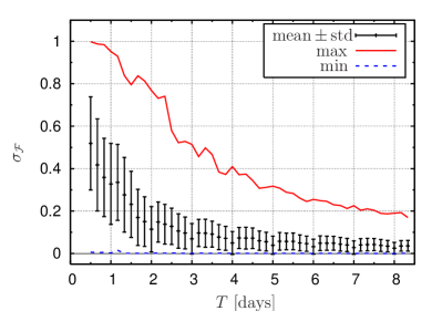
Refer to caption
Figure 3: Distribution of the relative intrinsic uncertainty σsubscript𝜎\sigma_{\mathcal{F}} of the \mathcal{F}-mismatch as a function of observation time T𝑇T, for the single-detector case. Plotted are the mean, standard deviation and extremal values of the distribution for each value of T𝑇T.

Fig. 3 shows the distribution of the relative uncertainty σ(λ,Δλ)subscript𝜎𝜆Δ𝜆\sigma_{\mathcal{F}}({\lambda},\Delta{\lambda}), as a function of the observation time T𝑇T for randomly chosen signal parameters and offsets (using the algorithm described in Sect. IV.3). These results are for the single-detector case only, the corresponding dependence on the number of detectors is investigated in Sect. IV.6. We see in Fig. 3 that for short observation times, of the order of T12similar-to𝑇12T\sim 12 hours, the relative uncertainty can be as large as 100%percent100100\%. For longer observation times of the order of a few days, σsubscript𝜎\sigma_{\mathcal{F}} decreases substantially, but even for T8similar-to𝑇8T\sim 8 days, the intrinsic uncertainty can still reach up to about 202020 %.

IV.5 Comparing different metric approximations

For the following comparisons of different metric approximations, it will be useful to define the relative error ε(a,b)𝜀𝑎𝑏\varepsilon(a,b) between two quantities a𝑎a and b𝑏b as

ε(a,b)ab(|a|+|b|)/2,𝜀𝑎𝑏𝑎𝑏𝑎𝑏2\varepsilon(a,b)\equiv{a-b\over(|a|+|b|)/2}\,, (135)

which is the harmonic mean of (ab)/|a|𝑎𝑏𝑎(a-b)/|a| and (ab)/|b|𝑎𝑏𝑏(a-b)/|b|. This definition has the advantage of being bound within [2,2]22[-2,2] even for large deviations abmuch-greater-than𝑎𝑏a\gg b or bamuch-greater-than𝑏𝑎b\gg a, while it agrees with the more common definitions of relative errors for small values |ε|1much-less-than𝜀1|\varepsilon|\ll 1.

IV.5.1 Monte-Carlo study of mismatches

As we have seen in Fig. 3, the intrinsic relative uncertainty σsubscript𝜎\sigma_{\mathcal{F}} decreases substantially on the timescale of a few days, corresponding to a convergence gijg¯ijsubscriptsuperscript𝑔𝑖𝑗subscriptsuperscript¯𝑔𝑖𝑗g^{\mathcal{F}}_{ij}\rightarrow\overline{g}^{\mathcal{F}}_{ij}. The average metric g¯ijsubscriptsuperscript¯𝑔𝑖𝑗\overline{g}^{\mathcal{F}}_{ij} is therefore expected to be an increasingly reliable approximation of the full \mathcal{F}-metric gijsubscriptsuperscript𝑔𝑖𝑗g^{\mathcal{F}}_{ij} with longer observation times T𝑇T.

Refer to caption
Figure 4: Distribution of relative errors ε(m,m¯)𝜀subscript𝑚subscript¯𝑚\varepsilon(m_{\mathcal{F}},\overline{m}_{\mathcal{F}}) of the (single-detector) average \mathcal{F}-mismatch m¯subscript¯𝑚\overline{m}_{\mathcal{F}} with respect to the exact \mathcal{F}-mismatch msubscript𝑚m_{\mathcal{F}} as a function of observation time T𝑇T. Plotted are the mean, standard deviation and extremal values of the distribution for each value of T𝑇T.

This is indeed the case, as can be seen in Fig. 4, which shows the distribution of relative errors ε(m,m¯)𝜀subscript𝑚subscript¯𝑚\varepsilon(m_{\mathcal{F}},\,\overline{m}_{\mathcal{F}}) as a function of observation time T𝑇T. This distribution was obtained using random choices of the signal parameters and Doppler offsets as described in Sect. IV.3. The standard deviation of the relative errors is about 2020~{}20 % for short observation times T1less-than-or-similar-to𝑇1T\lesssim 1 day, but rapidly decreases to about 111 % for timescales of a few days. Note that these errors are somewhat smaller than could have been expected from the intrinsic uncertainty σsubscript𝜎\sigma_{\mathcal{F}} shown in Fig. 3, which indicates that mismatches near the extremal values mmin|maxsuperscriptsubscript𝑚conditionalminmaxm_{\mathcal{F}}^{{\mathrm{min}}|{\mathrm{max}}} are less likely than those closer to the average m¯subscript¯𝑚\overline{m}_{\mathcal{F}}.

As shown in Sect. III.5, the \mathcal{F}-metric family gijsubscriptsuperscript𝑔𝑖𝑗g^{\mathcal{F}}_{ij} converges to the orbital metric gijorbsubscriptsuperscript𝑔orb𝑖𝑗g^{\mathrm{orb}}_{ij} for very long observation times T1much-greater-than𝑇1T\gg 1 day, but it is not obvious on which timescales this convergence happens in practice.
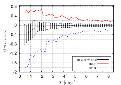
Refer to caption
Figure 5: Distribution of relative errors ε(m,morb)𝜀subscript𝑚subscript𝑚orb\varepsilon(m_{\mathcal{F}},m_{\mathrm{orb}}) of the orbital metric with respect to the (single-detector) \mathcal{F}-metric as a function of observation time T𝑇T. Plotted are the mean, standard deviation and extremal values of the distribution for each value of T𝑇T.

Fig. 5 shows the relative errors ε(m,morb)𝜀subscript𝑚subscript𝑚orb\varepsilon(m_{\mathcal{F}},m_{\mathrm{orb}}) of the orbital metric compared to the exact \mathcal{F}-metric, as a function of observation time. Note that a plot with the distribution of ε(m,mϕ)𝜀subscript𝑚subscript𝑚italic-ϕ\varepsilon(m_{\mathcal{F}},m_{\phi}) would look virtually indistinguishable.
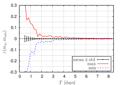
Refer to caption
Figure 6: Distribution of relative errors ε(mϕ,morb)𝜀subscript𝑚italic-ϕsubscript𝑚orb\varepsilon(m_{\phi},m_{\mathrm{orb}}) of the orbital metric with respect to the phase metric as a function of observation time T𝑇T. Plotted are the mean, standard deviation and extremal values of the distribution for each value of T𝑇T.

These two metric approximations perform nearly identically as far as predicting mismatches is concerned, as can be seen in Fig. 6 showing the distribution of relative errors ε(mϕ,morb)𝜀subscript𝑚italic-ϕsubscript𝑚orb\varepsilon(m_{\phi},m_{\mathrm{orb}}). Note that the orbital as well as the phase metric show a tendency to overestimate the mismatch for short observation times T1less-than-or-similar-to𝑇1T\lesssim 1 days, which is apparent in Fig. 5. Summarizing, we conclude that the “mismatch quality” of the orbital and of the phase metric seem virtually identical, and both approximations perform only sightly worse than the average \mathcal{F}-metric shown in Fig. 4. However, as will become clear in the next section, there is an important difference between the phase metric and the orbital metric, which does not manifest itself in this Monte-Carlo study due to the smallness of the relevant parameter space in which the difference becomes apparent.

IV.5.2 Metric determinants and eigenvalues

A complementary way of comparing different metrics is to look at their eigenvalues and determinants. These invariant quantities characterize the semi-major axes and the volume of iso-mismatch hyperellipsoids, which are important properties for the template covering of the parameter space. We denote the four metric eigenvalues as g1g2g3g4subscript𝑔1subscript𝑔2subscript𝑔3subscript𝑔4g_{1}\geq g_{2}\geq g_{3}\geq g_{4}. The metric for isolated neutron-star signals is quite generally represented by highly ill-conditioned matrices in the default parameter-space coordinates (α,δ,f,f˙,𝛼𝛿𝑓˙𝑓\alpha,\delta,f,{\dot{f}},...). That means that g1subscript𝑔1g_{1} is typically many orders of magnitude larger than g4subscript𝑔4g_{4}, corresponding to very thin and elongated mismatch hyperellipsoids. This property can be characterized by the so-called condition number, defined as κg1/g4𝜅subscript𝑔1subscript𝑔4\kappa\equiv{g_{1}/g_{4}}. Well-conditioned matrices have κ𝒪(1)similar-to𝜅𝒪1\kappa\sim\mathcal{O}(1), while the metrics encountered here typically have κ(gij)1020similar-to𝜅subscriptsuperscript𝑔𝑖𝑗superscript1020\kappa(g^{\mathcal{F}}_{ij})\sim 10^{20} in SI units, and κ(gij^)108similar-to𝜅subscriptsuperscript𝑔^𝑖𝑗superscript108\kappa(g^{\mathcal{F}}_{\widehat{ij}})\sim 10^{8} in natural units (cf. Sect. IV.2). Ill-conditioned matrices can strongly amplify numerical errors in computing their maps, inverses, determinants or eigenvalues. One has to be very careful when handling such matrices numerically, as the results can be quite unreliable. Using SI units, it turns out to be all but impossible to compute the determinant or the eigenvalues using standard double-precision arithmetic, which suffers from complete loss of significant digits in this case. In natural units, however, these quantities can be computed (albeit not with good precision, and not for all points in parameter space), and the results for one example are shown in Fig. 7 and Fig. 8.
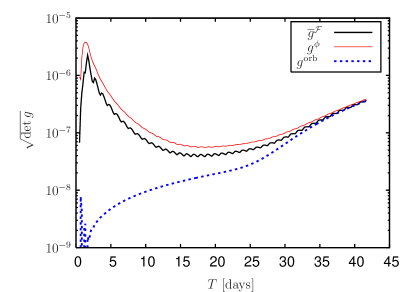
Refer to caption
Figure 7: Determinants of different metric approximations (in natural units) as functions of observation time T𝑇T. [Parameters: f=100𝑓100f=100 Hz, f˙=0˙𝑓0{\dot{f}}=0, α=1.0rad𝛼1.0rad\alpha=1.0~{}\textrm{rad}, δ=0.5rad𝛿0.5rad\delta=0.5~{}\textrm{rad}, detector = ’H1’, GPS start-time t0=792576013subscript𝑡0792576013t_{0}=792576013 s]

Contrary to the apparent fast convergence of the orbital- and the \mathcal{F}-mismatches shown in Fig. 5, we see a very different picture for the metric determinants in Fig. 7.
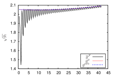
Refer to caption Refer to caption

Figure 8: Square roots of the four eigenvalues gisubscript𝑔𝑖g_{i} of different metric approximations (in natural units) as functions of observation time T𝑇T. [Same parameters as in Fig. 7]

For timescales of a few days, the determinant of the orbital metric is a few orders of magnitude smaller than the determinants of the other metric approximations, and the expected convergence (118) takes place only for timescales longer than T1greater-than-or-equivalent-to𝑇1T\gtrsim 1 month.

How can this be reconciled with the apparently much faster convergence of the mismatches in Fig. 5? In order to better understand this, let us look at the four eigenvalues gisubscript𝑔𝑖g_{i} as functions of T𝑇T, which is shown in Fig. 8. We see that the largest discrepancy of the orbital metric occurs for the smallest eigenvalue, g4subscript𝑔4g_{4}, corresponding to the most degenerate direction of the metric. The largest two eigenvalues g1,g2subscript𝑔1subscript𝑔2g_{1},g_{2} agree well, and g3subscript𝑔3g_{3} only differs by a factor of a few. In order for the mismatch to be affected by the smallest eigenvalue, we would have to pick a Doppler offset that is very closely aligned with the most degenerate principal axis, as any appreciable offset along the other axes would easily dominate the total mismatch. A very rough order-of-magnitude estimate of the probability p𝑝p of picking such a direction yields an upper bound of p(g4/g1)(g4/g2)(g4/g3)106less-than-or-similar-to𝑝subscript𝑔4subscript𝑔1subscript𝑔4subscript𝑔2subscript𝑔4subscript𝑔3less-than-or-similar-tosuperscript106p\lesssim\sqrt{(g_{4}/g_{1})(g_{4}/g_{2})(g_{4}/g_{3})}\lesssim 10^{-6}. It is therefore very unlikely to pick a Doppler offset for which the mismatch is dominated by the smallest eigenvalue. This is consistent with the fact that in about 105similar-toabsentsuperscript105\sim 10^{5} trials we did not see any cases in which the orbital metric had dramatically underestimated the mismatch, i.e. where ε(m,morb)2similar-to𝜀subscript𝑚subscript𝑚orb2\varepsilon(m_{\mathcal{F}},m_{\mathrm{orb}})\sim 2 in Fig. 5.

It is interesting to note that while the phase metric seems virtually identical to the orbital metric for “almost all” directions in parameter space, its determinant (and eigenvalues) agree much better with the (average) \mathcal{F}-metric. The small effect of the spin motion of the earth is negligible for most directions in parameter space, except for the most degenerate one, where it substantially reduces the degeneracy.

IV.6 The multi-detector \mathcal{F}-metric

As discussed in Sect. III.3, the parameter-space resolution of the multi-detector \mathcal{F}-metric does not scale with the number of detectors. Instead, the effect of combining detectors coherently results in a noise-weighted average of contributions from different detectors. This averaging operation (59) would be expected to decrease the effects of the antenna-pattern functions aX(t)superscript𝑎X𝑡a^{\mathrm{X}}(t) and bX(t)superscript𝑏X𝑡b^{\mathrm{X}}(t), as well as the detector-specific Doppler modulation ΔϕX(t)Δsuperscriptitalic-ϕX𝑡\Delta\phi^{\mathrm{X}}(t) of the signal phase (108).

(a)Refer to caption (b)Refer to caption

Figure 9: Distribution of (a) intrinsic relative \mathcal{F}-metric uncertainty σsubscript𝜎\sigma_{\mathcal{F}} and (b) relative errors ε(m,morb)𝜀subscript𝑚subscript𝑚orb\varepsilon(m_{\mathcal{F}},m_{\mathrm{orb}}) as functions of the coherent combination of (assumed equal-noise) detectors, for T=55𝑇55T=55 hours. Plotted are the mean, standard deviation and extremal values of the distribution for each detector combination. The assumed detectors (location and orientation only) are: ’H1’ = LIGO Hanford, ’L1’ = LIGO Livingston, ’G1’ = GEO600, ’V1’ = Virgo, ’T1’ = TAMA, ’P1’ = Caltech 40m.

In Fig. 9 we see indeed that both the intrinsic uncertainty σsubscript𝜎\sigma_{\mathcal{F}} of the \mathcal{F}-metric family, as well as its relative difference to the orbital metric decrease with the number of detectors. These results are based on a Monte-Carlo simulation with 40,000similar-toabsent40000\sim 40,000 randomly chosen parameters (see Sect. IV.3), for a fixed observation time of T=55𝑇55T=55 hours, and using between one and six coherently combined detectors. For the sake of this example, we have made the (obviously unrealistic) assumption that all 6 detectors have the same noise floor, otherwise the convergence would be much weaker. Note that we would find exactly the same mismatch convergence for the phase metric as that shown in Fig. 9(b) for the orbital metric.

IV.7 Comparing metric predictions to measured mismatches

In order to validate the theoretical \mathcal{F}-statistic mismatch msubscript𝑚m_{\mathcal{F}}, derived in Sect. III.2, we compare it to the measured relative SNR loss m0subscript𝑚0m_{0} in a simulated mismatched search. This is done by first generating (using lalapps_Makefakedata LIGO Scientific Collaboration ) a fake signal with parameters {𝒜,λs}𝒜subscript𝜆s\{{\mathcal{A}},{\lambda}_{\mathrm{s}}\} picked at random (see Sect. IV.3). We then measure (using lalapps_ComputeFStatistic LIGO Scientific Collaboration ) the perfectly-matched SNR ρ(0)𝜌0\rho(0) at the signal location λssubscript𝜆s{\lambda}_{\mathrm{s}}, and the mismatched SNR ρ(Δλ)𝜌Δ𝜆\rho(\Delta{\lambda}) at an offset Doppler position λs+Δλsubscript𝜆sΔ𝜆{\lambda}_{\mathrm{s}}+\Delta{\lambda}. The offsets ΔλΔ𝜆\Delta{\lambda} were picked at random using the algorithm described in Sect. IV.3. The measured \mathcal{F}-mismatch m0subscript𝑚0m_{0} is then given simply by the definition Eq. (46). The comparison of the measured mismatches m0subscript𝑚0m_{0} to the theoretical approximation reveals a problem with the metric approximation for large angular offsets (in natural units), in particular for ΔΩ^5greater-than-or-equivalent-toΔ^Ω5{\Delta\widehat{\Omega}}\gtrsim 5. The origin of this “metric failure” can be understood in terms of the metric curvature and will be discussed in more detail in IV.7.2. In the meantime we simply remove this known source of errors by excluding points with ΔΩ^>5Δ^Ω5{\Delta\widehat{\Omega}}>5, which affects less than 1%percent11\% of the Monte-Carlo trials.

(a)Refer to caption (b)Refer to caption

Figure 10: Measured mismatches m0subscript𝑚0m_{0} versus predicted \mathcal{F}-mismatches msubscript𝑚m_{\mathcal{F}} for observations times of (a) T=12𝑇12T=12 hours and (b) T=60𝑇60T=60 hours, omitting points with ΔΩ^>5Δ^Ω5{\Delta\widehat{\Omega}}>5. The dashed line indicates the identity function.

Fig. 10 shows the measured mismatches m0subscript𝑚0m_{0} as a function of the prediction msubscript𝑚m_{\mathcal{F}}, for observation times of (a) T=12𝑇12T=12 hours and (b) T=60𝑇60T=60 hours. We see that there is a substantial scattering of measured mismatches in the case of T=12𝑇12T=12 hours, which has virtually disappeared for T=60𝑇60T=60 hours. This second type of “metric failure”, which only affects short observation times, will be discussed in IV.7.1.

Another effect seen in these figures is a systematic deviation of m0subscript𝑚0m_{0} with respect to msubscript𝑚m_{\mathcal{F}} with increasing mismatches, which becomes noticeable at around m0.15greater-than-or-equivalent-tosubscript𝑚0.15m_{\mathcal{F}}\gtrsim 0.15. This deviation would be suspected due to higher-order corrections 𝒪(Δλ3)𝒪Δsuperscript𝜆3\mathcal{O}(\Delta\lambda^{3}) with respect to the local metric expansion, and is found to be roughly independent of the observation time T𝑇T. We can approximate this systematic deviation by an empirical quadratic correction of the form

m,qu(m)=m0.38m2,subscript𝑚qusubscript𝑚subscript𝑚0.38superscriptsubscript𝑚2m_{\mathcal{F},{\mathrm{qu}}}(m_{\mathcal{F}})=m_{\mathcal{F}}-0.38\,m_{\mathcal{F}}^{2}\,, (136)

which can be used in comparisons to measured mismatches, as it compensates for the systematic “drift” in m0subscript𝑚0m_{0}. Note that this deviation makes the metric a conservative over-estimate, as the actual mismatches tend to be smaller than the predicted ones.

IV.7.1 Metric problems for T1less-than-or-similar-to𝑇1T\lesssim 1 day

The strong scattering of mismatches seen in Fig. 10(a) for short observation times can be attributed to an intrinsic property of the \mathcal{F}-statistic: namely, the “local” parameter-space structure for short observation times is not very well approximated by a quadratic form in offsets. Note that obviously the metric approximation is valid in the strict local sense of sufficiently small offsets, but in practice we are more interested in a finite “local” region of small mismatches, m0.5less-than-or-similar-to𝑚0.5m\lesssim 0.5 say.

Refer to caption
Figure 11: Comparison of the measured decrease in \mathcal{F}-statistic (CFS) as a function of frequency offset ΔfΔ𝑓\Delta f, and the corresponding metric prediction 1m1subscript𝑚1-m_{\mathcal{F}}, for an observation time of T=5𝑇5T=5 hours. [Parameters: f=100𝑓100f=100 Hz, cosι=0.95𝜄0.95\cos\iota=0.95, ψ=2.25𝜓2.25\psi=2.25, α=5.98𝛼5.98\alpha=5.98, δ=0.09𝛿0.09\delta=0.09, f˙=0˙𝑓0{\dot{f}}=0]
Refer to caption
Figure 12: Same as Fig. 11 for an observation time of T=30𝑇30T=30 hours.

An illustrative example for this is shown in Figs. 11, 12, where we have measured the \mathcal{F}-statistic (using lalapps_ComputeFStatistic) over a 104similar-toabsentsuperscript104\sim 10^{-4} Hz band around the true signal frequency, with the other Doppler parameters (α,δ,f˙𝛼𝛿˙𝑓\alpha,\delta,{\dot{f}}) held fixed at their correct values. For an observation time of T=5𝑇5T=5 hours, the quadratic decrease predicted by the \mathcal{F}-metric is clearly not a good approximation, as can be seen in Fig. 11: depending on the sign of the frequency offset, the metric would either substantially under- or overestimate the mismatch. This effect decreases rapidly with observation time, and for T=30𝑇30T=30 hours (and the same signal), the decrease of the \mathcal{F}-statistic is “locally” much better approximated by the metric, as seen in Fig. 12. This effect can be understood as follows: the quadratic decrease of the \mathcal{F}-statistic predicted by the metric has a typical width in frequency of Δf01/Tsimilar-toΔsubscript𝑓01𝑇\Delta f_{0}\sim 1/T (cf. Sect. IV.2). However, the spin motion of the earth creates “side-lobes” in frequency space at offsets of a few fspin=1/f_{\mathrm{spin}}=1/day105similar-toabsentsuperscript105\sim 10^{-5} Hz, which are clearly visible in Fig. 12. For observation times much smaller than a day, these side-lobes are therefore not well separated from the main peak and will substantially alter its quadratic form, e.g. by creating “plateaus” and steeper “cliffs”, as seen in Fig. 11. As the observation time gets longer, i.e. T1greater-than-or-equivalent-to𝑇1T\gtrsim 1 day, the main peak becomes well separated, and therefore well described by the metric approximation.

IV.7.2 Metric problems for ΔΩ^>5Δ^Ω5{\Delta\widehat{\Omega}}>5

As already mentioned, another problem with the metric approximation affects points with large angular offsets ΔΩ^Δ^Ω{\Delta\widehat{\Omega}}, and is present even for long observation times. This can be seen in Fig. 13, showing the relative errors ε(m0,m,qu)𝜀subscript𝑚0subscript𝑚qu\varepsilon(m_{0},m_{\mathcal{F},{\mathrm{qu}}}) as a function of angular offset ΔΩ^Δ^Ω{\Delta\widehat{\Omega}}, for observation times T>48𝑇48T>48 hours.

Refer to caption
Figure 13: Relative errors ε(m0,m,qu)𝜀subscript𝑚0subscript𝑚qu\varepsilon(m_{0},m_{\mathcal{F},{\mathrm{qu}}}) versus angular offset ΔΩ^Δ^Ω{\Delta\widehat{\Omega}} in natural units, for observation times T>48𝑇48T>48 hours. For better readability of the figure, the displayed range of angular offsets is limited to ΔΩ^40Δ^Ω40{\Delta\widehat{\Omega}}\leq 40.

For angular offsets ΔΩ^<5Δ^Ω5{\Delta\widehat{\Omega}}<5, the relative errors stay below ε(m0,m,qu)<0.1𝜀subscript𝑚0subscript𝑚qu0.1\varepsilon(m_{0},m_{\mathcal{F},{\mathrm{qu}}})<0.1, but with increasing ΔΩ^Δ^Ω{\Delta\widehat{\Omega}}, the errors start to spread out substantially.

The reason for this metric failure can be traced to the curvature of the metric on the sky. While the metric ellipses have constant orientation as functions of frequency and spindown, their orientation changes with sky position. This curvature is closely related to the global “circles in the sky” (CiS) structure discussed in Prix and Itoh (2005), as the metric ellipses on the sky are “tangential” to these circles. To first order, the CiS are described by the equation

f(1+nV/c)=fs(1+nsV/c),𝑓1𝑛𝑉𝑐subscript𝑓s1subscript𝑛s𝑉𝑐f\left(1+{\vec{n}}\cdot\vec{V}/c\right)=f_{\mathrm{s}}\left(1+{\vec{n}}_{\mathrm{s}}\cdot\vec{V}/c\right)\,, (137)

where f𝑓f and n𝑛{\vec{n}} are the “target” frequency and sky position respectively, while fssubscript𝑓sf_{\mathrm{s}} and nssubscript𝑛s{\vec{n}}_{\mathrm{s}} are the corresponding signal parameters.
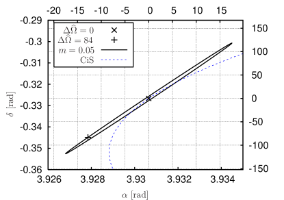
Refer to caption
Figure 14: Metric “failure” for large angular offset ΔΩ^=84Δ^Ω84{\Delta\widehat{\Omega}}=84 at T=68𝑇68T=68 hours. The point ’x’ indicates the signal location, ’+’ shows an offset location on the m=0.05𝑚0.05m=0.05 iso-mismatch ellipse with a measured mismatch of m01similar-tosubscript𝑚01m_{0}\sim 1. The dashed line indicates the “circle in the sky” (137) defined by the signal location. The top and right-hand axes show the offsets in natural units. [Parameters: f=186.34𝑓186.34f=186.34 Hz, α=3.93𝛼3.93\alpha=3.93, δ=0.33𝛿0.33\delta=-0.33, f˙=1.7×10¹⁰s2˙𝑓1.7superscript1010superscript𝑠2{\dot{f}}=1.7\times 10^{-10}s^{-2}, cosι=0.4𝜄0.4\cos\iota=0.4, ψ=1.65𝜓1.65\psi=1.65 ]

The problem stems from the curvature of the \mathcal{F}-statistic circles in the sky-coordinates α𝛼\alpha, δ𝛿\delta, which is why the CiS is only locally well approximated by the respective mismatch ellipses. This effect is seen clearly in Fig. 14, which shows an extreme example of such a metric “failure” due to large ΔΩ^Δ^Ω{\Delta\widehat{\Omega}}. In this figure, ’+’ indicates a sky position on the m=0.05subscript𝑚0.05m_{\mathcal{F}}=0.05 iso-mismatch ellipse, which has an angular offset from the signal of ΔΩ^=84Δ^Ω84{\Delta\widehat{\Omega}}=84. Contrary to the predicted mismatch, the measured mismatch at this point is m01similar-tosubscript𝑚01m_{0}\sim 1, as the \mathcal{F}-statistic decreases rapidly away from the CiS (indicated by the dashed line).

IV.7.3 Summary of metric validation

Fig. 15 summarizes the relative errors ε(m0,m,qu)𝜀subscript𝑚0subscript𝑚qu\varepsilon(m_{0},m_{\mathcal{F},{\mathrm{qu}}}) between the (quadratically corrected) predictions (136) and the measured mismatches m0subscript𝑚0m_{0}, as a function of observation time T𝑇T.

Refer to caption

Figure 15: Distribution of relative errors ε(m0,m,qu)𝜀subscript𝑚0subscript𝑚qu\varepsilon(m_{0},m_{\mathcal{F},{\mathrm{qu}}}) as a function of observation time T𝑇T. Plotted are the mean, standard deviation and extremal values of the distribution for each value of T𝑇T, excluding points with ΔΩ^>5Δ^Ω5{\Delta\widehat{\Omega}}>5. The points ’x’ and ’+’ indicate the respective maximum and minimum errors when including results with ΔΩ^>5Δ^Ω5{\Delta\widehat{\Omega}}>5.

We see that, as expected, excluding large angular offsets (ΔΩ^>5Δ^Ω5{\Delta\widehat{\Omega}}>5) yields a substantially improved agreement between the metric prediction and the measurements, as it eliminates the type of “metric failures” discussed in IV.7.2. We also see that the relative errors can still be quite large for short observation times T1less-than-or-similar-to𝑇1T\lesssim 1 day, as discussed in IV.7.1, and that these errors decrease rapidly with T𝑇T. For observation times of T1greater-than-or-equivalent-to𝑇1T\gtrsim 1 day, the average error is below a few percent. We can therefore conclude that the agreement of the \mathcal{F}-metric with the measurements is very good in the domain of applicability of the metric approximation.

V Discussion

We have derived a formalism for the general parameter-space metric of the multi-detector \mathcal{F}-statistic, and we have explicitly computed the metric for signals from isolated spinning neutron stars. We have shown that there exists a family of \mathcal{F}-metrics, parametrized by the two (unknown) amplitude parameters ψ𝜓\psi and cosι𝜄\cos\iota. We explicitly derived the extremal “mismatch bounds” (i.e. the maximum and minimum possible mismatches) of the \mathcal{F}-metric family, and we introduced an average \mathcal{F}-metric, which is independent of the unknown amplitude parameters. We have shown that the multi-detector \mathcal{F}-metric does not scale with the number of detectors. Combining detectors coherently therefore does not increase the required number of templates. In the long-duration limit (T1greater-than-or-equivalent-to𝑇1T\gtrsim 1 month), we found that the \mathcal{F}-metric family converges towards a simple orbital metric gijorbsubscriptsuperscript𝑔orb𝑖𝑗g^{\mathrm{orb}}_{ij}, which neglects both the amplitude modulation and the phase modulation caused by the diurnal rotation of the Earth.

Both the orbital and the closely related phase metric provide relatively good mismatch approximations in practice, and the quality of these approximations improves with longer observation times and with the number of coherently-combined detectors.

The orbital metric, however, while virtually identical to the phase metric for almost all directions in parameter space, was found to be substantially more degenerate for observation times shorter than a month. This has important consequences for the covering problem of the parameter space and requires further study. Finally, we have identified two regimes in which the local metric approximation itself is not very reliable: namely, for observation times T1less-than-or-similar-to𝑇1T\lesssim 1 day, and for large angular offsets ΔΩ^5greater-than-or-equivalent-toΔ^Ω5{\Delta\widehat{\Omega}}\gtrsim 5 (in natural units).

Appendix A Alternative derivation of the \mathcal{F}-metric

A more elegant derivation of the \mathcal{F}-metric (47) can be obtained Cutler by projecting the full parameter-space metric in {𝒜,λ}𝒜𝜆\{{\mathcal{A}},{\lambda}\} into the reduced parameter space λ𝜆{\lambda} of the \mathcal{F}-statistic. We denote the full parameter space as θ={𝒜,λ}𝜃𝒜𝜆\theta=\{{\mathcal{A}},{\lambda}\}, and we use index conventions θa={𝒜μ,λi}superscript𝜃𝑎superscript𝒜𝜇superscript𝜆𝑖\theta^{a}=\{\mathcal{A}^{\mu},\lambda^{i}\}. Recall the form of the log-likelihood ratio (15), namely

lnΛ(𝒙;θ)(𝒙|𝒔(θ))12(𝒔(θ)|𝒔(θ)).Λ𝒙𝜃conditional𝒙𝒔𝜃12conditional𝒔𝜃𝒔𝜃\ln\Lambda(\mathchoice{\mbox{\boldmath$\displaystyle x$}}{\mbox{\boldmath$\textstyle x$}}{\mbox{\boldmath$\scriptstyle x$}}{\mbox{\boldmath$\scriptscriptstyle x$}};\theta)\equiv\left(\mathchoice{\mbox{\boldmath$\displaystyle x$}}{\mbox{\boldmath$\textstyle x$}}{\mbox{\boldmath$\scriptstyle x$}}{\mbox{\boldmath$\scriptscriptstyle x$}}|\mathchoice{\mbox{\boldmath$\displaystyle s$}}{\mbox{\boldmath$\textstyle s$}}{\mbox{\boldmath$\scriptstyle s$}}{\mbox{\boldmath$\scriptscriptstyle s$}}(\theta)\right)-{1\over 2}\left(\mathchoice{\mbox{\boldmath$\displaystyle s$}}{\mbox{\boldmath$\textstyle s$}}{\mbox{\boldmath$\scriptstyle s$}}{\mbox{\boldmath$\scriptscriptstyle s$}}(\theta)|\mathchoice{\mbox{\boldmath$\displaystyle s$}}{\mbox{\boldmath$\textstyle s$}}{\mbox{\boldmath$\scriptstyle s$}}{\mbox{\boldmath$\scriptscriptstyle s$}}(\theta)\right)\,. (138)

If the data contains a signal with parameters θssubscript𝜃s\theta_{\mathrm{s}}, i.e. 𝒙(t)=𝒏(t)+𝒔(t;θs)𝒙𝑡𝒏𝑡𝒔𝑡subscript𝜃s\mathchoice{\mbox{\boldmath$\displaystyle x$}}{\mbox{\boldmath$\textstyle x$}}{\mbox{\boldmath$\scriptstyle x$}}{\mbox{\boldmath$\scriptscriptstyle x$}}(t)=\mathchoice{\mbox{\boldmath$\displaystyle n$}}{\mbox{\boldmath$\textstyle n$}}{\mbox{\boldmath$\scriptstyle n$}}{\mbox{\boldmath$\scriptscriptstyle n$}}(t)+\mathchoice{\mbox{\boldmath$\displaystyle s$}}{\mbox{\boldmath$\textstyle s$}}{\mbox{\boldmath$\scriptstyle s$}}{\mbox{\boldmath$\scriptscriptstyle s$}}(t;\theta_{\mathrm{s}}), and if the target position θ𝜃\theta is “close” to the signal location, i.e. θ=θs+Δθ𝜃subscript𝜃sΔ𝜃\theta=\theta_{\mathrm{s}}+\Delta\theta for “small” ΔθΔ𝜃\Delta\theta, then the expectation value of lnΛΛ\ln\Lambda can be expanded as

2E[lnΛ(θ|θs)]=(𝒔|𝒔)(a𝒔|b𝒔)ΔθaΔθb+𝒪(3),2𝐸delimited-[]Λconditional𝜃subscript𝜃sconditional𝒔𝒔conditionalsubscript𝑎𝒔subscript𝑏𝒔Δsuperscript𝜃𝑎Δsuperscript𝜃𝑏𝒪32E\left[\ln\Lambda(\theta|\theta_{\mathrm{s}})\right]=\left(\mathchoice{\mbox{\boldmath$\displaystyle s$}}{\mbox{\boldmath$\textstyle s$}}{\mbox{\boldmath$\scriptstyle s$}}{\mbox{\boldmath$\scriptscriptstyle s$}}|\mathchoice{\mbox{\boldmath$\displaystyle s$}}{\mbox{\boldmath$\textstyle s$}}{\mbox{\boldmath$\scriptstyle s$}}{\mbox{\boldmath$\scriptscriptstyle s$}}\right)-\left(\partial_{a}\mathchoice{\mbox{\boldmath$\displaystyle s$}}{\mbox{\boldmath$\textstyle s$}}{\mbox{\boldmath$\scriptstyle s$}}{\mbox{\boldmath$\scriptscriptstyle s$}}|\partial_{b}\mathchoice{\mbox{\boldmath$\displaystyle s$}}{\mbox{\boldmath$\textstyle s$}}{\mbox{\boldmath$\scriptstyle s$}}{\mbox{\boldmath$\scriptscriptstyle s$}}\right)\Delta\theta^{a}\Delta\theta^{b}+\mathcal{O}(3)\,, (139)

so the full parameter-space metric g~absubscript~𝑔𝑎𝑏\widetilde{g}_{ab} is found as

g~ab=(a𝒔|b𝒔)(𝒔|𝒔).subscript~𝑔𝑎𝑏conditionalsubscript𝑎𝒔subscript𝑏𝒔conditional𝒔𝒔\widetilde{g}_{ab}={(\partial_{a}\mathchoice{\mbox{\boldmath$\displaystyle s$}}{\mbox{\boldmath$\textstyle s$}}{\mbox{\boldmath$\scriptstyle s$}}{\mbox{\boldmath$\scriptscriptstyle s$}}|\partial_{b}\mathchoice{\mbox{\boldmath$\displaystyle s$}}{\mbox{\boldmath$\textstyle s$}}{\mbox{\boldmath$\scriptstyle s$}}{\mbox{\boldmath$\scriptscriptstyle s$}})\over(\mathchoice{\mbox{\boldmath$\displaystyle s$}}{\mbox{\boldmath$\textstyle s$}}{\mbox{\boldmath$\scriptstyle s$}}{\mbox{\boldmath$\scriptscriptstyle s$}}|\mathchoice{\mbox{\boldmath$\displaystyle s$}}{\mbox{\boldmath$\textstyle s$}}{\mbox{\boldmath$\scriptstyle s$}}{\mbox{\boldmath$\scriptscriptstyle s$}})}\,. (140)

This expression is sometimes referred to as the normalized Fisher matrix Królak et al. (2004). As mentioned in the introduction, this “canonical” metric differs from a definition often found in the literature (e.g. Owen (1996); Balasubramanian et al. (1996); Cornish and Porter (2005)), which is based on a somewhat more ad-hoc measure of the “match”, namely M(s(θs)|s(θ))𝑀conditional𝑠subscript𝜃s𝑠𝜃M\equiv\left(s(\theta_{\mathrm{s}})|s(\theta)\right), instead of the full log-likelihood (138). As it turns out, both definitions result in the same phase metric (119) when considering constant-amplitude signals (after minimizing the mismatch (140) over the unknown amplitude). In general, however, the canonical definition (140), and correspondingly (46), is more directly relevant to the covering problem, as it describes the relative loss of detection statistic. For the assumed general form of the signal (1), we have

ρ2(0)(𝒔|𝒔)=𝒜μμν𝒜ν,superscript𝜌20conditional𝒔𝒔superscript𝒜𝜇subscript𝜇𝜈superscript𝒜𝜈\rho^{2}(0)\equiv(\mathchoice{\mbox{\boldmath$\displaystyle s$}}{\mbox{\boldmath$\textstyle s$}}{\mbox{\boldmath$\scriptstyle s$}}{\mbox{\boldmath$\scriptscriptstyle s$}}|\mathchoice{\mbox{\boldmath$\displaystyle s$}}{\mbox{\boldmath$\textstyle s$}}{\mbox{\boldmath$\scriptstyle s$}}{\mbox{\boldmath$\scriptscriptstyle s$}})=\mathcal{A}^{\mu}\mathcal{M}_{\mu\nu}\mathcal{A}^{\nu}\,, (141)

and the respective derivatives with respect to the amplitude and Doppler subspaces are given by

μ𝒔subscript𝜇𝒔\displaystyle\partial_{\mu}\mathchoice{\mbox{\boldmath$\displaystyle s$}}{\mbox{\boldmath$\textstyle s$}}{\mbox{\boldmath$\scriptstyle s$}}{\mbox{\boldmath$\scriptscriptstyle s$}} =\displaystyle= 𝒔Aμ=𝒉μ(t;λ),𝒔superscript𝐴𝜇subscript𝒉𝜇𝑡𝜆\displaystyle{\partial\mathchoice{\mbox{\boldmath$\displaystyle s$}}{\mbox{\boldmath$\textstyle s$}}{\mbox{\boldmath$\scriptstyle s$}}{\mbox{\boldmath$\scriptscriptstyle s$}}\over\partial A^{\mu}}=\mathchoice{\mbox{\boldmath$\displaystyle h$}}{\mbox{\boldmath$\textstyle h$}}{\mbox{\boldmath$\scriptstyle h$}}{\mbox{\boldmath$\scriptscriptstyle h$}}_{\mu}(t;{\lambda})\,, (142)
i𝒔subscript𝑖𝒔\displaystyle\partial_{i}\mathchoice{\mbox{\boldmath$\displaystyle s$}}{\mbox{\boldmath$\textstyle s$}}{\mbox{\boldmath$\scriptstyle s$}}{\mbox{\boldmath$\scriptscriptstyle s$}} =\displaystyle= 𝒔λi=𝒜μi𝒉μ.𝒔superscript𝜆𝑖superscript𝒜𝜇subscript𝑖subscript𝒉𝜇\displaystyle{\partial\mathchoice{\mbox{\boldmath$\displaystyle s$}}{\mbox{\boldmath$\textstyle s$}}{\mbox{\boldmath$\scriptstyle s$}}{\mbox{\boldmath$\scriptscriptstyle s$}}\over\partial\lambda^{i}}=\mathcal{A}^{\mu}\,\partial_{i}\mathchoice{\mbox{\boldmath$\displaystyle h$}}{\mbox{\boldmath$\textstyle h$}}{\mbox{\boldmath$\scriptstyle h$}}{\mbox{\boldmath$\scriptscriptstyle h$}}_{\mu}\,. (143)

The full metric g~absubscript~𝑔𝑎𝑏\widetilde{g}_{ab} therefore consists of the three blocks (with respect to the two subspaces):

g~ab=ρ2(0)(μν𝒜νμνi𝒜νμνi𝒜αhαβij𝒜β),subscript~𝑔𝑎𝑏superscript𝜌20subscript𝜇𝜈superscript𝒜𝜈subscript𝜇𝜈𝑖superscript𝒜𝜈subscript𝜇𝜈𝑖superscript𝒜𝛼subscript𝛼𝛽𝑖𝑗superscript𝒜𝛽\widetilde{g}_{ab}=\rho^{-2}(0)\,\left(\begin{array}[]{c c}\mathcal{M}_{\mu\nu}&\mathcal{A}^{\nu}\mathcal{R}_{\mu\nu i}\\[2.84544pt] \mathcal{A}^{\nu}\mathcal{R}_{\mu\nu i}&\mathcal{A}^{\alpha}h_{\alpha\beta ij}\mathcal{A}^{\beta}\\ \end{array}\right)\,, (144)

in terms of hijsubscript𝑖𝑗h_{ij} and isubscript𝑖\mathcal{R}_{i} defined in (40) and (31). The \mathcal{F}-metric gijsubscriptsuperscript𝑔𝑖𝑗g^{\mathcal{F}}_{ij} in the Doppler subspace can be regarded as the distance corresponding to given Doppler offsets Δθi=ΔλiΔsuperscript𝜃𝑖Δsuperscript𝜆𝑖\Delta\theta^{i}=\Delta\lambda^{i}, minimized over the amplitude offsets Δθμ=Δ𝒜μΔsuperscript𝜃𝜇Δsuperscript𝒜𝜇\Delta\theta^{\mu}=\Delta\mathcal{A}^{\mu}, i.e.

gijΔλiΔλjsubscriptsuperscript𝑔𝑖𝑗Δsuperscript𝜆𝑖Δsuperscript𝜆𝑗\displaystyle g^{\mathcal{F}}_{ij}\,\Delta\lambda^{i}\,\Delta\lambda^{j} \displaystyle\equiv minΔ𝒜μg~abΔθaΔθb.subscriptminΔsuperscript𝒜𝜇subscript~𝑔𝑎𝑏Δsuperscript𝜃𝑎Δsuperscript𝜃𝑏\displaystyle{\mathrm{min}}_{\Delta\!\mathcal{A}^{\mu}}\,\widetilde{g}_{ab}\,\Delta\theta^{a}\,\Delta\theta^{b}\,. (145)

This can be minimized trivially, since it is a quadratic function in Δ𝒜μΔsuperscript𝒜𝜇\Delta\mathcal{A}^{\mu}, and the “compensating” amplitude mismatches are

Δθμ=g^μνg~νiΔθi,Δsuperscript𝜃𝜇superscript^𝑔𝜇𝜈subscript~𝑔𝜈𝑖Δsuperscript𝜃𝑖\Delta\theta^{\mu}=-\widehat{g}^{\mu\nu}\,\widetilde{g}_{\nu i}\,\Delta\theta^{i}\,, (146)

where g^μνsuperscript^𝑔𝜇𝜈\widehat{g}^{\mu\nu} is the inverse matrix of g~μνsubscript~𝑔𝜇𝜈\widetilde{g}_{\mu\nu}, i.e. g^μαg~αν=δνμsuperscript^𝑔𝜇𝛼subscript~𝑔𝛼𝜈subscriptsuperscript𝛿𝜇𝜈\widehat{g}^{\mu\alpha}\widetilde{g}_{\alpha\nu}=\delta^{\mu}_{\nu}. Inserting this into (145) we obtain

gij=g~ijg~iμg^μνg~νj,subscriptsuperscript𝑔𝑖𝑗subscript~𝑔𝑖𝑗subscript~𝑔𝑖𝜇superscript^𝑔𝜇𝜈subscript~𝑔𝜈𝑗g^{\mathcal{F}}_{ij}=\widetilde{g}_{ij}-\widetilde{g}_{i\mu}\widehat{g}^{\mu\nu}\widetilde{g}_{\nu j}\,, (147)

which corresponds to the projection of the full metric g~absubscript~𝑔𝑎𝑏\widetilde{g}_{ab} into the Doppler subspace. Using the explicit components (144), we find

gij(𝒜)superscriptsubscript𝑔𝑖𝑗𝒜\displaystyle g_{ij}^{\mathcal{F}}({\mathcal{A}}) =\displaystyle= ρ2(0)𝒜[hij1Tij]𝒜superscript𝜌20𝒜delimited-[]subscript𝑖𝑗superscriptsubscriptsuperscript1𝑖Tsubscript𝑗𝒜\displaystyle\rho^{-2}(0)\,{\mathcal{A}}\left[h_{ij}-\mathcal{R}{{}^{\mathrm{T}}\!}_{i}\mathcal{M}^{-1}\mathcal{R}_{j}\right]{\mathcal{A}} (148)
=\displaystyle= 𝒜𝒢ij𝒜𝒜𝒜,𝒜subscript𝒢𝑖𝑗𝒜𝒜𝒜\displaystyle{{\mathcal{A}}\cdot\mathcal{G}_{ij}\cdot{\mathcal{A}}\over{\mathcal{A}}\cdot\mathcal{M}\cdot{\mathcal{A}}}\,, (149)

in perfect agreement with the earlier result (48), which was obtained in a more straightforward, but somewhat more tedious calculation.

Appendix B \mathcal{F}-metric for low-frequency signals

In the case of low frequencies fssubscript𝑓sf_{\mathrm{s}} (which would be relevant for LISA) and/or short observation times T𝑇T, where fsT≫̸104not-much-greater-thansubscript𝑓s𝑇superscript104f_{\mathrm{s}}\,T\not\gg 10^{4}, we cannot use the simplifying approximation of Sect. III.4. We can nevertheless proceed in the same way: using the expansion (64) and keeping only leading-order terms, we can express (40) as

hμνijsubscript𝜇𝜈𝑖𝑗\displaystyle h_{\mu\nu\,ij} \displaystyle\approx 12𝒮1T(Pij1Pij30Pij4Pij3Pij2Pij400Pij4Pij1Pij3Pij40Pij3Pij2),12superscript𝒮1𝑇subscriptsuperscript𝑃1𝑖𝑗subscriptsuperscript𝑃3𝑖𝑗0subscriptsuperscript𝑃4𝑖𝑗subscriptsuperscript𝑃3𝑖𝑗subscriptsuperscript𝑃2𝑖𝑗subscriptsuperscript𝑃4𝑖𝑗00subscriptsuperscript𝑃4𝑖𝑗subscriptsuperscript𝑃1𝑖𝑗subscriptsuperscript𝑃3𝑖𝑗subscriptsuperscript𝑃4𝑖𝑗0subscriptsuperscript𝑃3𝑖𝑗subscriptsuperscript𝑃2𝑖𝑗\displaystyle{1\over 2}\mathcal{S}^{-1}T\,\left(\begin{array}[]{c c c c}P^{1}_{ij}&P^{3}_{ij}&0&P^{4}_{ij}\\ P^{3}_{ij}&P^{2}_{ij}&-P^{4}_{ij}&0\\ 0&-P^{4}_{ij}&P^{1}_{ij}&P^{3}_{ij}\\ P^{4}_{ij}&0&P^{3}_{ij}&P^{2}_{ij}\\ \end{array}\right)\,, (154)

in terms of the four independent components

Pij1=iajaS+a2iϕjϕS,Pij2=ibjbS+b2iϕjϕS,Pij3=iajbS+abiϕjϕS,Pij4=biajϕSaibjϕS,subscriptsuperscript𝑃1𝑖𝑗subscriptdelimited-⟨⟩subscript𝑖𝑎subscript𝑗𝑎𝑆subscriptdelimited-⟨⟩superscript𝑎2subscript𝑖italic-ϕsubscript𝑗italic-ϕ𝑆subscriptsuperscript𝑃2𝑖𝑗subscriptdelimited-⟨⟩subscript𝑖𝑏subscript𝑗𝑏𝑆subscriptdelimited-⟨⟩superscript𝑏2subscript𝑖italic-ϕsubscript𝑗italic-ϕ𝑆subscriptsuperscript𝑃3𝑖𝑗subscriptdelimited-⟨⟩subscript𝑖𝑎subscript𝑗𝑏𝑆subscriptdelimited-⟨⟩𝑎𝑏subscript𝑖italic-ϕsubscript𝑗italic-ϕ𝑆subscriptsuperscript𝑃4𝑖𝑗subscriptdelimited-⟨⟩𝑏subscript𝑖𝑎subscript𝑗italic-ϕ𝑆subscriptdelimited-⟨⟩𝑎subscript𝑖𝑏subscript𝑗italic-ϕ𝑆\begin{array}[]{rcl}P^{1}_{ij}&=&{{\langle\partial_{i}a\,\partial_{j}a\rangle}_{\!S}}+{{\langle a^{2}\,\partial_{i}\phi\,\partial_{j}\phi\rangle}_{\!S}}\,,\\[2.84544pt] P^{2}_{ij}&=&{{\langle\partial_{i}b\,\partial_{j}b\rangle}_{\!S}}+{{\langle b^{2}\,\partial_{i}\phi\,\partial_{j}\phi\rangle}_{\!S}}\,,\\[2.84544pt] P^{3}_{ij}&=&{{\langle\partial_{i}a\,\partial_{j}b\rangle}_{\!S}}+{{\langle a\,b\,\partial_{i}\phi\,\partial_{j}\phi\rangle}_{\!S}}\,,\\[2.84544pt] P^{4}_{ij}&=&{{\langle b\,\partial_{i}a\,\partial_{j}\phi\rangle}_{\!S}}-{{\langle a\,\partial_{i}b\,\partial_{j}\phi\rangle}_{\!S}}\,,\\ \end{array} (155)

with implicit symmetrization in i,j𝑖𝑗i,j. In a similar manner we calculate μνisubscript𝜇𝜈𝑖\mathcal{R}_{\mu\nu\,i}, defined in (31), which yields

μνi12𝒮1T(^i~i~i^i),subscript𝜇𝜈𝑖12superscript𝒮1𝑇subscript^𝑖subscript~𝑖subscript~𝑖subscript^𝑖\mathcal{R}_{\mu\nu\,i}\approx{1\over 2}\mathcal{S}^{-1}T\,\left(\begin{array}[]{c c}\widehat{\mathcal{R}}_{i}&\widetilde{\mathcal{R}}_{i}\\ -\widetilde{\mathcal{R}}_{i}&\widehat{\mathcal{R}}_{i}\\ \end{array}\right)\,, (156)

where the 2x2 matrices ^isubscript^𝑖\widehat{\mathcal{R}}_{i} and ~isubscript~𝑖\widetilde{\mathcal{R}}_{i} are defined as

^i(Ri11Ri12Ri21Ri22),and~i(Ri13Ri14Ri14Ri24),formulae-sequencesubscript^𝑖subscriptsuperscript𝑅11𝑖subscriptsuperscript𝑅12𝑖subscriptsuperscript𝑅21𝑖subscriptsuperscript𝑅22𝑖andsubscript~𝑖subscriptsuperscript𝑅13𝑖subscriptsuperscript𝑅14𝑖subscriptsuperscript𝑅14𝑖subscriptsuperscript𝑅24𝑖\widehat{\mathcal{R}}_{i}\equiv\left(\begin{array}[]{c c}R^{11}_{i}&R^{12}_{i}\\ R^{21}_{i}&R^{22}_{i}\\ \end{array}\right)\,,\;\textrm{and}\;\widetilde{\mathcal{R}}_{i}\equiv\left(\begin{array}[]{c c}R^{13}_{i}&R^{14}_{i}\\ R^{14}_{i}&R^{24}_{i}\\ \end{array}\right)\,, (157)

in terms of

Ri11=aiaS,Ri12=aibS,Ri21=biaS,Ri22=bibS,Ri13=a2iϕS,Ri24=b2iϕS,Ri14=abiϕS.formulae-sequencesuperscriptsubscript𝑅𝑖11subscriptdelimited-⟨⟩𝑎subscript𝑖𝑎𝑆superscriptsubscript𝑅𝑖12subscriptdelimited-⟨⟩𝑎subscript𝑖𝑏𝑆formulae-sequencesuperscriptsubscript𝑅𝑖21subscriptdelimited-⟨⟩𝑏subscript𝑖𝑎𝑆superscriptsubscript𝑅𝑖22subscriptdelimited-⟨⟩𝑏subscript𝑖𝑏𝑆formulae-sequencesuperscriptsubscript𝑅𝑖13subscriptdelimited-⟨⟩superscript𝑎2subscript𝑖italic-ϕ𝑆superscriptsubscript𝑅𝑖24subscriptdelimited-⟨⟩superscript𝑏2subscript𝑖italic-ϕ𝑆superscriptsubscript𝑅𝑖14subscriptdelimited-⟨⟩𝑎𝑏subscript𝑖italic-ϕ𝑆\begin{array}[]{c}R_{i}^{11}={{\langle a\,\partial_{i}a\rangle}_{\!S}}\,,\quad R_{i}^{12}={{\langle a\,\partial_{i}b\rangle}_{\!S}}\,,\\[2.84544pt] R_{i}^{21}={{\langle b\,\partial_{i}a\rangle}_{\!S}}\,,\quad R_{i}^{22}={{\langle b\,\partial_{i}b\rangle}_{\!S}}\,,\\[2.84544pt] R_{i}^{13}={{\langle a^{2}\partial_{i}\phi\rangle}_{\!S}}\,,\quad R_{i}^{24}={{\langle b^{2}\partial_{i}\phi\rangle}_{\!S}}\,,\\[2.84544pt] R_{i}^{14}={{\langle a\,b\,\partial_{i}\phi\rangle}_{\!S}}\,.\\ \end{array} (158)

Note that R^isubscript^𝑅𝑖\widehat{R}_{i} only contains derivatives of the antenna-pattern functions aXsuperscript𝑎Xa^{\mathrm{X}}, bXsuperscript𝑏Xb^{\mathrm{X}} (which where neglected in Sect. III.4), while R~isubscript~𝑅𝑖\widetilde{R}_{i} only contains derivatives of the phase. As a consequence of this block structure, one finds

{iT1j}μν12𝒮1T(Qij1Qij30Qij4Qij3Qij2Qij400Qij4Qij1Qij3Qij40Qij3Qij2),subscriptsuperscriptsubscript𝑖Tsuperscript1subscript𝑗𝜇𝜈12superscript𝒮1𝑇superscriptsubscript𝑄𝑖𝑗1superscriptsubscript𝑄𝑖𝑗30superscriptsubscript𝑄𝑖𝑗4superscriptsubscript𝑄𝑖𝑗3superscriptsubscript𝑄𝑖𝑗2superscriptsubscript𝑄𝑖𝑗400superscriptsubscript𝑄𝑖𝑗4superscriptsubscript𝑄𝑖𝑗1superscriptsubscript𝑄𝑖𝑗3superscriptsubscript𝑄𝑖𝑗40superscriptsubscript𝑄𝑖𝑗3superscriptsubscript𝑄𝑖𝑗2\left\{{{}^{\mathrm{T}}\!}\mathcal{R}_{i}\mathcal{M}^{-1}\mathcal{R}_{j}\right\}_{\mu\nu}\approx{1\over 2}\mathcal{S}^{-1}T\left(\begin{array}[]{c c c c}Q_{ij}^{1}&Q_{ij}^{3}&0&Q_{ij}^{4}\\ Q_{ij}^{3}&Q_{ij}^{2}&-Q_{ij}^{4}&0\\ 0&-Q_{ij}^{4}&Q_{ij}^{1}&Q_{ij}^{3}\\ Q_{ij}^{4}&0&Q_{ij}^{3}&Q_{ij}^{2}\\ \end{array}\right)\,, (159)

with the four independent components

DQij1=A[Ri21Rj21+Ri14Rj14]+B[Ri11Rj11+Ri13Rj13]2C[Ri11Rj21+Ri13Rj14],DQij2=A[Ri24Rj24+Ri22Rj22]+B[Ri14Rj14+Ri12Rj12]2C[Ri14Rj24+Ri12Rj22],DQij3=A[Ri14Rj24+Ri22Rj21]+B[Ri14Rj13+Ri12Rj11]C[Ri24Rj13+Ri14Rj14+Ri11Rj22+Ri12Rj21],DQij4=A[Ri21Rj24Ri14Rj22]+B[Ri11Rj14Ri12Rj13]C[Ri11Rj24Ri13Rj22+Ri14Rj21Ri12Rj14].𝐷subscriptsuperscript𝑄1𝑖𝑗𝐴delimited-[]subscriptsuperscript𝑅21𝑖subscriptsuperscript𝑅21𝑗subscriptsuperscript𝑅14𝑖subscriptsuperscript𝑅14𝑗𝐵delimited-[]subscriptsuperscript𝑅11𝑖subscriptsuperscript𝑅11𝑗subscriptsuperscript𝑅13𝑖subscriptsuperscript𝑅13𝑗missing-subexpressionmissing-subexpression2𝐶delimited-[]subscriptsuperscript𝑅11𝑖subscriptsuperscript𝑅21𝑗subscriptsuperscript𝑅13𝑖subscriptsuperscript𝑅14𝑗𝐷subscriptsuperscript𝑄2𝑖𝑗𝐴delimited-[]subscriptsuperscript𝑅24𝑖subscriptsuperscript𝑅24𝑗subscriptsuperscript𝑅22𝑖subscriptsuperscript𝑅22𝑗𝐵delimited-[]subscriptsuperscript𝑅14𝑖subscriptsuperscript𝑅14𝑗subscriptsuperscript𝑅12𝑖subscriptsuperscript𝑅12𝑗missing-subexpressionmissing-subexpression2𝐶delimited-[]subscriptsuperscript𝑅14𝑖subscriptsuperscript𝑅24𝑗subscriptsuperscript𝑅12𝑖subscriptsuperscript𝑅22𝑗𝐷subscriptsuperscript𝑄3𝑖𝑗𝐴delimited-[]subscriptsuperscript𝑅14𝑖subscriptsuperscript𝑅24𝑗subscriptsuperscript𝑅22𝑖subscriptsuperscript𝑅21𝑗𝐵delimited-[]subscriptsuperscript𝑅14𝑖subscriptsuperscript𝑅13𝑗subscriptsuperscript𝑅12𝑖subscriptsuperscript𝑅11𝑗missing-subexpressionmissing-subexpression𝐶delimited-[]subscriptsuperscript𝑅24𝑖subscriptsuperscript𝑅13𝑗subscriptsuperscript𝑅14𝑖subscriptsuperscript𝑅14𝑗subscriptsuperscript𝑅11𝑖subscriptsuperscript𝑅22𝑗subscriptsuperscript𝑅12𝑖subscriptsuperscript𝑅21𝑗𝐷subscriptsuperscript𝑄4𝑖𝑗𝐴delimited-[]subscriptsuperscript𝑅21𝑖subscriptsuperscript𝑅24𝑗subscriptsuperscript𝑅14𝑖subscriptsuperscript𝑅22𝑗𝐵delimited-[]subscriptsuperscript𝑅11𝑖subscriptsuperscript𝑅14𝑗subscriptsuperscript𝑅12𝑖subscriptsuperscript𝑅13𝑗missing-subexpressionmissing-subexpression𝐶delimited-[]subscriptsuperscript𝑅11𝑖subscriptsuperscript𝑅24𝑗subscriptsuperscript𝑅13𝑖subscriptsuperscript𝑅22𝑗subscriptsuperscript𝑅14𝑖subscriptsuperscript𝑅21𝑗subscriptsuperscript𝑅12𝑖subscriptsuperscript𝑅14𝑗\begin{array}[]{rcl}D\,Q^{1}_{ij}&=&A\left[R^{21}_{i}R^{21}_{j}+R^{14}_{i}R^{14}_{j}\right]+B\left[R^{11}_{i}R^{11}_{j}+R^{13}_{i}R^{13}_{j}\right]\\[2.84544pt] &&-2C\left[R^{11}_{i}R^{21}_{j}+R^{13}_{i}R^{14}_{j}\right]\,,\\[2.84544pt] D\,Q^{2}_{ij}&=&A\left[R^{24}_{i}R^{24}_{j}+R^{22}_{i}R^{22}_{j}\right]+B\left[R^{14}_{i}R^{14}_{j}+R^{12}_{i}R^{12}_{j}\right]\\[2.84544pt] &&-2C\left[R^{14}_{i}R^{24}_{j}+R^{12}_{i}R^{22}_{j}\right]\,,\\[2.84544pt] D\,Q^{3}_{ij}&=&A\left[R^{14}_{i}R^{24}_{j}+R^{22}_{i}R^{21}_{j}\right]+B\left[R^{14}_{i}R^{13}_{j}+R^{12}_{i}R^{11}_{j}\right]\\[2.84544pt] &&-C\left[R^{24}_{i}R^{13}_{j}+R^{14}_{i}R^{14}_{j}+R^{11}_{i}R^{22}_{j}+R^{12}_{i}R^{21}_{j}\right]\,,\\[2.84544pt] D\,Q^{4}_{ij}&=&A\left[R^{21}_{i}R^{24}_{j}-R^{14}_{i}R^{22}_{j}\right]+B\left[R^{11}_{i}R^{14}_{j}-R^{12}_{i}R^{13}_{j}\right]\\[2.84544pt] &&-C\left[R^{11}_{i}R^{24}_{j}-R^{13}_{i}R^{22}_{j}+R^{14}_{i}R^{21}_{j}-R^{12}_{i}R^{14}_{j}\right]\,.\end{array} (160)

Putting all the pieces together, we find 𝒢ijsubscript𝒢𝑖𝑗\mathcal{G}_{ij}, defined in (44), in the form:

𝒢μν12𝒮1T(m1m30m4m3m2m400m4m1m3m40m3m2),subscript𝒢𝜇𝜈12superscript𝒮1𝑇superscript𝑚1superscript𝑚30superscript𝑚4superscript𝑚3superscript𝑚2superscript𝑚400superscript𝑚4superscript𝑚1superscript𝑚3superscript𝑚40superscript𝑚3superscript𝑚2\displaystyle\mathcal{G}_{\mu\nu}\approx{1\over 2}\mathcal{S}^{-1}T\,\left(\begin{array}[]{c c c c}m^{1}&m^{3}&0&m^{4}\\ m^{3}&m^{2}&-m^{4}&0\\ 0&-m^{4}&m^{1}&m^{3}\\ m^{4}&0&m^{3}&m^{2}\\ \end{array}\right)\,, (165)

in terms of the four components (r=1,2,3,4𝑟1234r=1,2,3,4):

mr(PijrQijr)ΔλiΔλj.superscript𝑚𝑟subscriptsuperscript𝑃𝑟𝑖𝑗subscriptsuperscript𝑄𝑟𝑖𝑗Δsuperscript𝜆𝑖Δsuperscript𝜆𝑗m^{r}\equiv\left(P^{r}_{ij}-Q^{r}_{ij}\right)\,\Delta\lambda^{i}\Delta\lambda^{j}\,. (166)

As discussed in Sect. III, the extrema m^subscript^𝑚{\widehat{m}}_{\mathcal{F}} are the eigenvalues of 1𝒢superscript1𝒢\mathcal{M}^{-1}\cdot\mathcal{G}, which are the solutions of

00\displaystyle 0 =\displaystyle= det1det[𝒢m^],superscript1delimited-[]𝒢subscript^𝑚\displaystyle\det\mathcal{M}^{-1}\,\det\left[\mathcal{G}-{\widehat{m}}_{\mathcal{F}}\,\mathcal{M}\right]\,, (167)

or equivalently

00\displaystyle 0 =\displaystyle= (m1m^A)(m2m^B)superscript𝑚1subscript^𝑚𝐴superscript𝑚2subscript^𝑚𝐵\displaystyle(m^{1}-{\widehat{m}}_{\mathcal{F}}A)(m^{2}-{\widehat{m}}_{\mathcal{F}}B) (168)
(m3m^C)2(m4)2.superscriptsuperscript𝑚3subscript^𝑚𝐶2superscriptsuperscript𝑚42\displaystyle\hskip 40.00006pt-(m^{3}-{\widehat{m}}_{\mathcal{F}}C)^{2}-(m^{4})^{2}\,.

We see that there are again maximally two independent eigenvalues, namely

m^max|min(λ;Δλ)=m¯±m¯2m~2,superscriptsubscript^𝑚conditionalmaxmin𝜆Δ𝜆plus-or-minussubscript¯𝑚superscriptsubscript¯𝑚2superscript~𝑚2{\widehat{m}}_{\mathcal{F}}^{{\mathrm{max}}|{\mathrm{min}}}({\lambda};\Delta{\lambda})=\overline{m}_{\mathcal{F}}\pm\sqrt{\overline{m}_{\mathcal{F}}^{2}-{\widetilde{m}}^{2}}\,, (169)

with

m¯=(2D)1[Bm1+Am22Cm3],m~=D1[m1m2(m3)2(m4)2],subscript¯𝑚superscript2𝐷1delimited-[]𝐵superscript𝑚1𝐴superscript𝑚22𝐶superscript𝑚3~𝑚superscript𝐷1delimited-[]superscript𝑚1superscript𝑚2superscriptsuperscript𝑚32superscriptsuperscript𝑚42\begin{array}[]{rcl}\overline{m}_{\mathcal{F}}&=&(2D)^{-1}\left[Bm^{1}+Am^{2}-2Cm^{3}\right]\,,\\[2.84544pt] {\widetilde{m}}&=&D^{-1}\left[m^{1}m^{2}-(m^{3})^{2}-(m^{4})^{2}\right]\,,\\ \end{array} (170)

which is formally very similar to the earlier result (102).

Acknowledgements.
I am very grateful to Curt Cutler for numerous helpful suggestions, and I thank Chris Messenger, Andrzej Królak, Badri Krishnan and Ben Owen for useful discussions and comments.

References

  • Balasubramanian et al. (1996) R. Balasubramanian, B. S. Sathyaprakash, and S. V. Dhurandhar, Phys. Rev. D. 53, 3033 (1996).
  • Owen (1996) B. J. Owen, Phys. Rev. D. 53, 6749 (1996).
  • Apostolatos (1995) T. A. Apostolatos, Phys. Rev. D. 52, 605 (1995).
  • Królak et al. (2004) A. Królak, M. Tinto, and M. Vallisneri, Phys. Rev. D. 70, 022003 (2004).
  • Prix and Itoh (2005) R. Prix and Y. Itoh, Class. Quant. Grav. 22, S1003 (2005).
  • Prix et al. (LIGO Scientific Collaboration) R. Prix et al. (LIGO Scientific Collaboration), submitted (2006).
  • Jaranowski et al. (1998) P. Jaranowski, A. Królak, and B. F. Schutz, Phys. Rev. D. 58, 063001 (1998).
  • Abbott et al. (LIGO Scientific Collaboration) B. Abbott et al. (LIGO Scientific Collaboration), Phys. Rev. D. 69, 082004 (2004).
  • Abbott et al. (LIGO Scientific Collaboration) B. Abbott et al. (LIGO Scientific Collaboration), submitted (2006), eprint gr-qc/0605028.
  • Astone et al. (2005) P. Astone et al., Class. Quant. Grav. 22, 1243 (2005).
  • Cutler and Schutz (2005) C. Cutler and B. F. Schutz, Phys. Rev. D. 72, 063006 (2005).
  • Cornish and Porter (2005) N. J. Cornish and E. K. Porter, Class. Quant. Grav. 22, S927 (2005).
  • Brady et al. (1998) P. R. Brady, T. Creighton, C. Cutler, and B. F. Schutz, Phys. Rev. D. 57, 2101 (1998).
  • Jones et al. (2006) D. I. Jones, B. J. Owen, and D. Whitbeck, in preparation (2006).
  • (15) LIGO Scientific Collaboration, LAL/LALApps: FreeSoftware (GPL) tools for data-analysis., http://www.lsc-group.phys.uwm.edu/daswg/.
  • Finn (1992) L. S. Finn, Phys. Rev. D. 46, 5236 (1992).
  • Jaranowski and Królak (2005) P. Jaranowski and A. Królak, Living Reviews in Relativity 8, 3 (2005).
  • Pan et al. (2004) Y. Pan, A. Buonanno, Y. Chen, and M. Vallisneri, Phys. Rev. D. 69, 104017 (2004).
  • Buonanno et al. (2005) A. Buonanno, Y. Chen, Y. Pan, H. Tagoshi, and M. Vallisneri, Phys. Rev. D. 72, 084027 (2005).
  • (20) C. Cutler, private communication.