Detecting Highly Oscillatory Signals by Chirplet Path Pursuit

Abstract

This paper considers the problem of detecting nonstationary phenomena, and chirps in particular, from very noisy data. Chirps are waveforms of the very general form $A(t)\exp(\mathrm{i}\lambda\,\varphi(t))$, where $\lambda$ is a (large) base frequency, the phase $\varphi(t)$ is time-varying and the amplitude $A(t)$ is slowly varying. Given a set of noisy measurements, we would like to test whether there is signal or whether the data is just noise. One particular application of note in conjunction with this problem is the detection of gravitational waves predicted by Einstein’s Theory of General Relativity.

We introduce detection strategies which are very sensitive and more flexible than existing feature detectors. The idea is to use structured algorithms which exploit information in the so-called chirplet graph to chain chirplets together adaptively as to form chirps with polygonal instantaneous frequency. We then search for the path in the graph which provides the best trade-off between complexity and goodness of fit. Underlying our methodology is the idea that while the signal may be extremely weak so that none of the individual empirical coefficients is statistically significant, one can still reliably detect by combining several coefficients into a coherent chain. This strategy is general and may be applied in many other detection problems. We complement our study with numerical experiments showing that our algorithms are so sensitive that they seem to detect signals whenever their strength makes them detectable.

Keywords. Signal Detection, Nonparametric Testing, Likelihood Ratios, Adaptivity, Chirps, Chirplets, Time-Frequency Analysis, Gravitational Waves, Graphs, Shortest Path in a Graph, Dynamic Programming.

Acknowledgments. E. C. was partially supported by National Science Foundation grants DMS 01-40698 (FRG) and ITR ACI-0204932. P. C. was partially supported by NSF grant PHY-0107417. Many thanks to David Donoho, Houman Ohwadi, Justin Romberg and Chiara Sabatti for fruitful conversations. We would also like to thank Ery Arias-Castro for references. The results in this paper were first presented at “Regularization in Statistics,” Banff, Canada, September 2003 and at “Multiscale Geometric Analysis in High Dimensions,” UCLA, Los Angeles, California, November 2004 [9].

1 Introduction

This paper considers the problem of detecting one-dimensional signals from noisy measurements. Suppose we have noisy sampled data

$$y_{i}=\alpha\,S_{i}+z_{i},\qquad i=1,\ldots,N,$$ (1.1)

where the unknown vector $(S_{i})$ are sampled values $S_{i}=S(t_{i})$ of a signal of interest $S(t),t\in[0,1]$, and $(z_{i})$ is a zero-mean stochastic vector, not necessarily i.i.d. but with a known distribution. Based on the observations $(y_{i})$, one would like to decide whether or not a signal is hiding in the noise. Formally, we would like to test the null hypothesis

$$H_{0}:\alpha=0\mbox{ (noise only)}$$

against the alternative

$$H_{1}:\alpha\neq 0\mbox{ (signal is buried in noise)}.$$

We emphasize here is that the signal $S$ is completely unknown and may not depend upon a small number of parameters. This situation is commonly referred as nonparametric testing as opposed to the classical parametric setup where it is assumed that the set of candidate signals belong to a known parametric class.

1.1 Chirps

In this paper, we will focus our attention on the detection of frequency modulated signals also named ‘chirps.’ Roughly speaking, a chirp is a signal of the form

$$S(t)=A(t)\,\cos(\lambda\varphi(t)),$$ (1.2)

where the amplitude $A$ and the phase $\varphi$ are smoothly varying functions of time, and where the oscillation degree $\lambda$ is large. It follows from the definition that chirps are highly oscillatory signals with a frequency content $\omega(t)$ also rapidly changing over time; although this is an ill-defined concept, researchers like to talk about the ‘instantaneous frequency’ of a chirp simply defined as the derivative of the phase function

$$\omega(t)=\lambda\varphi^{\prime}(t).$$ (1.3)

(This definition can be justified in the case where $\lambda|\varphi^{\prime}(t)|^{2}/|\varphi^{\prime\prime}(t)|\gg 1$ and we skip the details [19].) Hence, for large values of $\lambda$, the frequency content of a chirping signal is also rapidly changing with time.

Chirps arise in a number of important scientific disciplines, including the analysis of Echolocation in Bats [25, 24] and other mammals [22], the study of atmospheric whistlers [15], and very recently, in efforts to detect gravitational waves [26, 4]. For example, a particular species of bats (Eptesicus fuscus) uses a remarkable sonar system for navigation in which some specific chirps are emitted. Because chirps are ubiquitous in nature, strategies for their detection are bound to be of great practical interest. We briefly mention two applications:

1. Remote sensing. Suppose that we have one or several objects moving in a cluttered background. In anti submarine warfare, for example, one would like to detect the presence of submarines from noisy acoustic data. Because different engines have different time-frequency characteristics, we would expect the signal at the sensor to behave like a chirp. In a more peaceful underwater setting, whales are known to emit chirping sounds [22] and their detection would help locating and/or tracking these mammals. If we could also estimate some basic characteristics of the chirp, then one could also discern between different types of submarines, or different species of whales.

   A closely related application is active ranging where one detects the location and velocity of objects by sending an electromagnetic wave and recording the echo. Because objects are moving, the Doppler effect implies that the recorded signal is chirp-like.

2. Detection of gravitational waves. Whereas the existence of gravitational waves was predicted long ago by the theory of general relativity, they have not been confirmed experimentally [26]. There are massive ongoing efforts aimed at detecting gravitational waves. Detecting gravitational waves on earth is very challenging because of the extremely tiny effects they induce on physical systems so that the signal is expected to be buried in a sea of noise. Interestingly, many gravitational waves are well-modeled by time-frequency modulated signals [4, 3].

1.2 Gravitational waves

In this short section, we briefly expand on the problem of detecting gravitational waves as this really is the main applicative focus of this line work, see the companion paper [10]. Predicted by Einstein’s General Theory of Relativity, gravitational waves are disturbances in the curvature of spacetime caused by the motions of matter. Expressed in a different way, they are oscillations propagating at the speed of light in the fabric of spacetime. A strong source of gravitational waves is a system made up of two massive objects closely and rapidly orbiting each other, e.g. two black holes, two neutron stars, etc. As they are orbiting, general relativity predicts that the system loses energy in the form of gravitational radiation, causing the objects to gradually spiral in towards each other, eventually resulting in a violent merger.

When a gravitational passes, it alternatively stretches and shrinks distances. The Laser Interferometric Gravitational-wave Observatory (LIGO) [1] is a sophisticated apparatus which uses interferometry to detect such variations (VIRGO is the European equivalent). The difficulty is that even strong sources will induce variations in an incredibly small scale: the variation is proportional to the length

$$\Delta L=hL,$$

where the factor $h$ is about $10^{-21}$. In LIGO, $L$ is the distance between two test masses and is about 4 kilometers so that one would need to detect a displacement of about $4\times 10^{-18}$ meters. This is a formidable challenge as this distance is about 1,000 times smaller than the nucleus of an atom! Because of many other sources of variations, the measurements of the displacements are expected to be extremely noisy.

Gravitational wave astronomy could offer a new window to the universe and expand our knowledge of the cosmos dramatically. Aside from demonstrating the existence of black holes and perhaps providing a wealth of data on supernovae and neutron stars, gravitational wave observations could revolutionize our view of the universe and unveil phenomena never considered before. We quote from Kip Throne, one of the leading LIGO scientists [1]: “Gravitational-wave detectors will soon bring us observational maps of black holes colliding […] and black holes thereby will become the objects of detailed scrutiny. What will that scrutiny teach us? There will be surprises.”

To see the relevance of our problem to gravitational wave detection, one can use Einstein’s equations to predict the shape of a wave. In the case of the coalescence of a binary system, the gravitational wave strain $S(t)$ (the relative displacement as a function of time) is approximately of the form

$$S(t)=A\cdot(t_{c}-t)^{-1/4}\,\cos(\omega\,(t-t_{c})^{5/8}+\phi),$$

where $A$ is a constant, $\omega$ is large and $t_{c}$ is the time of coalescence (merger); this approximation is only valid for $t<t_{c}$ and we do not know the shape of $S$ after the merger. Clearly, $S(t)$ is an example of a chirp. It is possible to push the calculations and add corrective terms to both the phase and amplitude [4, 3].

1.3 The challenges of chirp detection

While the literature on nonparametric estimation is fairly developed, that of nonparametric is perhaps more recent, see [16] and references therein. A typical assumption in nonparametric detection is to assume that the signal $S$ is smooth or does not vary too rapidly. For example, one could define a class of candidate signals by bounding the modulus of smoothness of $S$, or by imposing that $S$ lies in a ball taken from a smoothness class, e.g. a Sobolev or Besov type class. In this paper and specializing, (1.2), one might be interested in knowing whether or not a signal such as $S(t)=\cos(\pi Nt^{2}/2)$ for $t\in[0,1]$ is hiding in the data. If one collects samples at the equispaced time points $t_{i}=(i-1)/N$, then one can see that the signal changes sign at nearly the sampling rate (note that the frequency content is also changing at the sampling rate since the ‘instantaneous frequency’ increases linearly from $\omega=0$ to $\omega=\pi N$). With more generality, one could introduce a meaningful class of chirps of the form $A(t)\,\cos(N\varphi(t))$ by imposing the condition that $A$ and $\varphi$ have bounded higher order derivatives. The behavior of signals taken from such classes is very different than what is traditionally assumed in the literature. This the reason why the methodology we are about to introduce is also radically different.

Many of the methods envisioned for detecting gravitational waves heavily rely on very precise knowledge of the signal waveforms. The idea is to approximate the family of signals with a finite collection $\{S_{\theta}:\theta\in\Theta\}$ and perform a sort of generalized likelihood ratio test (GLRT) also known as the method of matched filters [21]. For example, in additive Gaussian white noise, one would compute $Z^{*}=\max_{\theta\in\Theta}\langle y,S_{\theta}\rangle/\|S_{\theta}\|$ and compare the value of the statistic with a fixed threshold. This methodology suffers from some severe problems such as prohibitive computational costs and lack or robustness resulting in poor detection methods where the waveforms are not well known. More to the point, this assumes that the unknown signal may be reduced to a finite set of templates so that the problem essentially reduces to a parametric test, which we are not willing to assume in this paper. Instead, and keeping Thorne’s comment in mind, one would like a robust and flexible methodology able to detect poorly modeled or even totally unknown but coherent signals.

1.4 Current detection strategies

In the last decade or so, various time-frequency methods have been proposed to overcome the problems with matched filters. For example, in [20], the proposal is to look for ridges in the time-scale plane. One computes the continuous time wavelet transform $W(a,b)$ where $a>0$ is scale and $b$ is time and search for a curve $\rho(a)$ along which the sum of $\int|W(a,\rho(a))|^{2}da/a$ is maximum. Because one cannot search the whole space of curves, the method is restricted to parametric ‘power-law chirps’ of the form $S(t)=(t_{0}-t)_{+}^{\alpha}\cos(2\pi F_{\beta}(t_{0}-t)^{\beta+1})$ where $\alpha$ and $\beta$ are unknown and $F_{\beta}$ is some constant. This is again a parametric problem. While the approach is more robust than the method of matched filters, it is also less sensitive. Among other issues, one problem is that the wavelet transform does not localize energy as much as one would want. In a similar fashion, [11] proposes to search for ridges in the time-frequency plane. Again, the methodology is designed for power-law chirps. The idea is to use appropriate time-frequency distributions such as the Wigner-Ville distribution (WVD) to localize the unknown signal as much as possible in the time-frequency plane. Here one needs, different time-frequency distributions for different chirp parameters $\alpha$ and $\beta$. For example the WVD is ideal for linear chirps but is ill-adapted to hyperbolic chirps, say, and one has to use another distribution. In practice, one also needs to deal with the undesirable interference properties of the WVD; to fix the interference methods requires ad-hoc methods which, in turn, have consequences on the sensitivity of the detector [11]. To summarize, while these methods may be more robust in parametric setups, they are also far less powerful.

As far as nonparametrics is concerned, [4] introduces a strategy where as before, the idea is to transform the data via the WVD giving the time frequency distribution $\rho(t,\omega)$, and then search for ridges (which is a problem similar to that of finding edges from very noisy image data). A decision is made whether or not each point in the time-frequency plane is a ‘ridge point,’ and the value of the statistical test depends on the length of the longest ridges. Again, because the WVD of a clean signal can take nonzero values in regions of the time-frequency plane having nothing to do with the spectral properties of the signal, one has to use a smoothing kernel to average the interference patterns, which simultaneously smears out the true ridges, thereby causing a substantial loss of resolution. Another issue with this approach is that while the signal may be detectable, it may not be locally detectable. This means that a huge majority of true ridge points may lie in the bulk of the data distribution, and not pass the threshold.

1.5 This paper

In this paper, we propose a detection strategy, which is very different than those currently employed in the literature. As explained earlier, we cannot hope to generate a family of chirps that would provide large correlations with the unknown signal; indeed, for a signal of size $N$, one would need to generate exponentially many waveforms which is unrealistic. But it is certainly possible to generate a family of templates which provide good local correlations, e.g. over shorter time intervals. We then build the so-called family of chirplets and our idea is to use a structured algorithm which exploit information in the family to chain chirplets together adaptively as to form a signal which is physically meaningful, and whose correlation with the data is largest. The basic strategy is as follows:

• We compute empirical coefficients by correlating the data with a family of templates which is rich enough to provide good local correlations with the unknown signal.

• We then exploit these empirical correlations and chain our coefficients in a meaningful way; i.e. so that the chain of ‘templates’ approximates a possible candidate signal.

• A possible detection strategy might then compare the sum of local correlations along the chain with a fixed threshold.

Of course, one would need to specify which templates one would want to use, which chaining rules one would want to allow, and how one should use this information to decide whether any signal is present or not. This is the subject of the remainder of this paper. But for now, observe that this is a general strategy. Suppose for simplicity that in the data model (1.1), the error terms are i.i.d. $N(0,\sigma^{2})$, and denote by $(f_{v})_{v\in V}$ our class of templates. One can think of our strategy as computing the individual $Z$-scores

$$Z_{v}=\langle y,f_{v}\rangle/\|f_{v}\|,\quad Z_{v}\sim N(\mu_{v},\sigma^{2}),$$

where $\mu_{v}=\alpha\langle S,f_{v}\rangle/\|f_{v}\|$, and then searching for a chain of templates such that the sum of the $Z$-scores is large. The key point here is that while the signal-to-noise ratio may be so low so that none of the individual $Z$ scores achieves statistical significance, $\mu_{v}\ll\sigma$ (i.e. the signal is there but not locally detectable), their sums along carefully selected paths would be judged statistically significant so that one could detect reliably.

We use the word ‘path’ because we have a graph structure in mind. In effect, we build a graph $G=(V,E)$ where the nodes $V$ correspond to our set of templates $(f_{v})_{v\in V}$ and the edges are connectivities between templates. The edges are chosen so that any path in the graph approximates a meaningful signal. The idea is to find a path which provides the best trade-off between correlation and complexity, where our measure of complexity is the number of templates used to fit the data.

Our methods are adaptive in the sense that they do not require any precise information about the phase and amplitude and yet, they are efficient at detecting a wide family of nonparametric alternatives. Our methods are also versatile and can accommodate many different types of noise distributions. For example, we will examine the case where the noise is Gaussian stationary with a known spectrum since this is the assumed noise distribution in gravitational wave detectors such as LIGO. Last but not least, our methods have remarkably low computational complexity, which is crucial for their effective deployment in applications.

1.6 Inspiration

Our methods are inspired by [14] where it was suggested that one could chain together beamlets to detect curves from noisy data. To the best of our knowledge, the idea of finding paths in a locally connected network to isolate salient features goes back to Sha’ashua and Ullman [23]. Closely related to this line of work is the more recent work [7] where a graph structure is used to detect filamentary structures. Having said that, the literature on the use of graphical models in signal detection is short. The detection strategies in this paper are different than those presented in the aforementioned references and are, therefore, adding to the developing literature. They can be applied to the problem of detecting chirps and gravitational waves in Astronomy but it is clear that they are also very general and can be tailored to address a variety of other statistical problems as well.

2 Multiscale Chirplets and the Chirplet Graph

2.1 Multiscale chirplets

This section introduces a family of multiscale chirplets which provide good local approximations of chirps under study. We assume we work in the time interval $[0,1]$ (and that our measurements are evenly sampled), and for each $j\geq 0$, we let $I$ denote the dyadic interval $I=[k2^{-j},(k+1)2^{-j}]$, where $k=0,1,\ldots,2^{j}-1$. We then define the multiscale chirplet dictionary as the family of functions defined by

$$f_{I,\mu}(t):=|I|^{-1/2}\,e^{\mathrm{i}(a_{\mu}t^{2}/2+b_{\mu}t)}\,1_{I}(t),$$ (2.1)

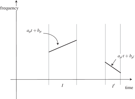
where $(a_{\mu},b_{\mu})\in{\cal M}_{j}$ is a discrete collection of offset and slope parameters which may depend on scale and on prior information about the objects of interest. We note that thanks to the normalization factor, chirplets are unit-normed, $\|f_{I,\mu}\|_{L_{2}}=1$. This system is appealing because a time-frequency portrait of its elements (say, by Wigner-Ville Distribution) reveals a system of elements of all possible durations, locations, average frequencies, and, most importantly, chirprates which are linear changes of instantaneous frequency during the interval of operation. Indeed, one can think of the ‘instantaneous frequency’ of a chirplet as being linear and equal to $a_{\mu}t+b_{\mu}$ so that in a diagrammatic sense, a chirplet is a segment in the time-frequency plane, see Figure 1.

Figure 1: Diagrammatic representation of two chirplets in the time-frequency plane.

Chirp atoms were introduced to deal with the nonstationary behavior of the instantaneous frequency of some signals. The terminology ‘chirplet’ is borrowed from the work of Mann and Haykin [18] (see also [8]) who have proposed the so-called chirplet transform of a signal: starting from the Gaussian multiparameter collection of linear chirps

$$g_{\lambda}(t)=g((t-b)/a)e^{\mathrm{i}(\omega t+\delta t^{2})},\quad\lambda=(a,b,\omega,\delta),$$ (2.2)

with $g$ a Gaussian window and $a>0$, and $b,\omega,\delta\in\mathbf{R}$, they define the chirplet transform of a signal $f$ as being the collection of inner products $c_{\lambda}=\langle f,g_{\lambda}\rangle$. The resemblance between (2.1) and (2.2) is self-evident—hence the terminology. What is new here is the notion of chirplet graph, which we will introduce below.

2.2 Discretization

We give a possible discretization for an evenly sampled signal of size $N=2^{J}$. For each dyadic interval $I=[k2^{-j},(k+1)2^{-j}]$, we mark out two vertical lines in the $[0,1]\times[-\pi,\pi]^{2}$ plane at the endpoints of $I$, $t_{I}=k2^{-j}$ and $t^{\prime}_{I}=(k+1)2^{-j}$, and place ticks along the vertical lines at spacing $2\pi/N$. We then create a dictionary of ‘chirplet lines’ connecting tick marks. For the simplicity of the exposition, suppose that the phase of the unknown chirp is such that we only have to create such lines with a slope—in absolute value—less or equal to $2\pi$. (This is suitable whenever $\lambda|\varphi^{\prime\prime}(t)|\leq 2\pi\,N$.) A simple count shows that the number of slopes is of size about $2N\cdot 2^{-j}$ so that the number $N_{j}$ of chirplets per dyadic interval obeys

$$N_{j}=\#\,\text{offsets }\times\#\,\text{slopes}\approx N\times 2N/2^{j}.$$

In other words, there are about

$$2^{j}\,N_{j}\asymp 2N^{2}$$

chirplets at scale $2^{-j}$. Thus, if we consider all scales $j=0,\ldots,\log_{2}(N)-1$, we see that the size of this special chirplet dictionary is about

$$2N^{2}\log_{2}N.$$

Of course, for evenly sampled signals, discrete chirplets are the sampled waveforms $f_{I,\mu}[t]=f_{I,\mu}((t-1)/N)/\sqrt{N}$, with $t=1,\ldots,N$. With the discrete chirplet dictionary in hand, we define the chirplet analysis or transform of a signal of length $N$ as the collection of inner products with all the elements in the dictionary. We call these inner products chirplet coefficients. It is clear that one can use the FFT to compute the chirplet coefficient table. For example, with the above discretization, it is possible to compute all the coefficients against chirplets ‘living’ in the fixed interval $[k2^{-j},(k+1)2^{-j})$ in $O(N_{j}\log(N/2^{j}))$ flops so that the computational complexity of the chirplet transform is $O(N^{2}\log^{2}N)$. There are many other possible discretizations and the experienced reader will also notice that for regular discretizations, the complexity will scale as $O(M_{N}\log N)$, where here and below $M_{N}$ is the number of chirplets in the dictionary. In summary, the computational cost is at most of the order $O(\log N)$ per chirplet coefficient.

2.3 The chirplet graph

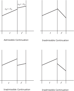
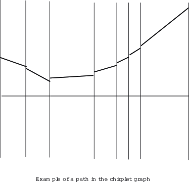
The main mathematical architecture of this paper is the chirplet graph $G=(V,E)$ where $V$ is the set of nodes and $E$ the set of edges. Each node in the graph is a chirplet index $v=(I,\mu)$. Throughout the paper, vertices corresponding to chirplets starting at time $t=0$ are said to be start-vertices, and vertices corresponding to chirplets ending at time $t=1$ are said to be end-vertices. The edges between vertices are selected to impose a certain regularity about the instantaneous frequency, see Figure 2.

(a)		(b)

Figure 2: (a) Example of connectivities in the chirplet graph. Chirplet may not be connected when the difference in offsets or slopes (or both) is large. (b) Diagrammatic representation of the instantaneous frequency along a path in the chirplet graph.

1. First, a natural constriction is that two chirplets can only be connected if they have adjacent supports in time.

2. Second, two chirplets are connected if the frequency offset at the juncture is small and if the difference in their slopes is not too large as well.

The idea is to model a chirp with instantaneous frequency $\lambda\varphi^{\prime}(t)$ as a sequence of connected line segments. Imposing constraints on the connectivities is akin to imposing constraints on the first derivative of the instantaneous frequency. With these definitions, a chirplet path is simply a set of connected vertices, starting from a start-vertex and ending at an end-vertex.

3 Detection Statistics

We now describe the complete algorithm for searching chirps through the data. To explain our methodology, it might be best first to focus on the case of additive Gaussian white noise

$$y_{i}=\alpha S_{i}+z_{i},\quad i=1,\ldots,N,\quad z_{i}\text{ i.i.d. }N(0,\sigma^{2}).$$

We wish to test $H_{0}:\alpha=0$ against $H_{1}:\alpha\neq 0$. A general strategy for testing composite hypotheses is the so-called Generalized Likelihood Ratio Test (GLRT). We suppose that the set of alternatives is of the form $\lambda f$ where $\lambda$ is a scalar and $f$ belongs to a subset ${\cal F}$ of unit vectors of $\mathbf{R}^{N}$, i.e. obeying $\|f\|=1$ for all $f\in{\cal F}$ (unless specified otherwise, $\|\cdot\|$ is the usual Euclidean norm). In other words, the alternative consists of multiples of a possibly exponentially large set of candidate signals. In this setup, the GLRT takes the form

$$\max_{\lambda\in\mathbf{R},f\in{\cal F}}\frac{L(\lambda f;y)}{L(0;y)},$$ (3.1)

where $L(\lambda f;y)$ is the likelihood of the data when the true mean vector is $\lambda f$. In the case of additive white noise, a simple calculation shows that the GLRT is proportional to

$$\max_{\lambda\in\mathbf{R},f\in{\cal F}}\,\,\,e^{-\|y-\lambda f\|^{2}/2\sigma^{2}}=\max_{f\in{\cal F}}\,\,\,e^{-\|y-\langle y,f\rangle f\|^{2}/2\sigma^{2}},$$

since for a fixed $f\in{\cal F}$, the likelihood is maximized for $\lambda=\langle y,f\rangle$. It then follows from Pythagoras’ identity $\|y-\langle y,f\rangle f\|^{2}=\|y\|^{2}-|\langle y,f\rangle|^{2}$ so that the GLRT is equivalent to finding the solution to

$$\max_{f\in{\cal F}}\,\,\,|\langle y,f\rangle|^{2},$$

and comparing this value with a threshold.

3.1 The Best Path statistic

Supplied with a chirplet graph, a reasonable strategy would be to consider the class of signals which can be rewritten as a superposition of piecewise linear chirps

$$f(t)=\sum_{v\in W}\lambda_{v}f_{v}(t),$$

where $W$ is any path in the chirplet graph and $(\lambda_{v})$ is any family of scalars, and apply the GLRT principle. In this setup, the GLRT is given by

$$\max_{W}\,\,\,\max_{(\lambda_{v})}\,\,\,e^{-\|y-\sum_{v\in W}\lambda_{v}f_{v}\|^{2}/2\sigma^{2}}=\max_{W}\,\,\,\max_{(\lambda_{v})}\,\,\,\prod_{v\in W}e^{-\|y_{v}-\lambda_{v}f_{v}\|^{2}/2\sigma^{2}},$$

where for each $v=(I,\mu)$, $y_{v}$ is the vector $(y_{t})_{t\in I}$, i.e. the portion of $y$ supported on the time interval $I$. Adapting the calculations detailed above shows that the GLRT is then equivalent to

$$\max_{W}\,\,\,\sum_{v\in W}|\langle y,f_{v}\rangle|^{2}.$$ (3.2)

In words, the GLRT simply finds the path in the chirplet graph which maximizes the sum of squares of the empirical coefficients. The major problem with this approach is that the GLRT will naively overfit the data. By choosing paths with shorter chirplets, one can find chirplets with increased correlations (one needs to match data on shorter intervals) and as a result, the sum $\sum_{v\in W}|\langle y,f_{v}\rangle|^{2}$ will increase. In the limit of tiny chirplets, $|\langle y,f_{v}\rangle|^{2}=\|y_{v}\|^{2}$ which gives

$$\max_{W}\,\,\,\sum_{v\in W}|\langle y,f_{v}\rangle|^{2}=\|y\|^{2},$$

and one has a perfect fit! There is an analogy with model selection in multiple regression where one improves the fit by increasing the number of predictors in the model. Just as in model selection, one needs to adjust the goodness of fit with the complexity of the fit.

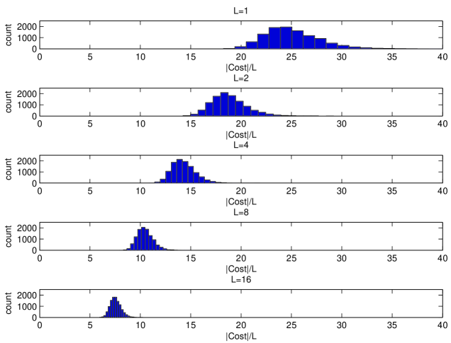
Let $W$ be a fixed path of length $|W|$. Then under the null hypothesis, $\sum_{v\in W}|\langle y,f_{v}\rangle|^{2}$ is distributed as a chi-squared random variable with $|W|$ degrees of freedom. Thus for fixed paths, we see that the value of the sum of squares along the path grows linearly with the length of the path. In some sense, the same conclusion applies to the maximal path; i.e. the value of the sum of squares along a path of a fixed size $\ell$ also grows approximately linearly with $\ell$, with a constant of proportionality greater than 1. An exact quantitative statement would be rather delicate to obtain in part because of the inherent complexity of the chirplet graph but also because it would need to depend on the special chirplet discretization. We refer the reader to [5].

The above analysis suggests taking a test statistic of the form

$$Z^{*}=\max_{W}\,\,\,\frac{\sum_{v\in W}|\langle y,f_{v}\rangle|^{2}}{|W|},$$ (3.3)

which may be seen as a perhaps unusual trade-off between the goodness of fit and the complexity of the fit. This is of course motivated by our heuristic argument which suggests that under the null hypothesis, the value of the best path of length $\ell$, that solution to

$$T^{*}_{\ell}:=\max_{|W|\leq\ell}\,\,\,\sum_{v\in W}|\langle y,f_{v}\rangle|^{2},$$ (3.4)

grows linearly with $\ell$, and is well concentrated around its mean by standard large deviation inequalities. In other words, with $Z^{*}_{\ell}:=T^{*}_{\ell}/\ell$, one would expect $Z^{*}_{\ell}$ to be about constant under $H_{0}$, at least for $\ell$ sufficiently large. This would imply that if we ignored paths of small length, one would expect—owing to sharp concentration—$Z^{*}=\max_{\ell}Z^{*}_{\ell}$ to be about constant under $H_{0}$. Therefore, a possible decision rule might be to reject $H_{0}$ if $Z^{*}$ is large.

Numerical simulations confirm that under the null, $T^{*}_{\ell}$ grows linearly with $\ell$ but they also show—as expected—deviations for small values of $\ell$, see Figure 3. For example, with the discretization discussed in Section 2.2, ${\hbox{\bf E}}Z^{*}_{\ell}$ seems to be decreasing with $\ell$. With this discretization, $Z^{*}$ is also almost all the time attained with paths of length 1 (one single chirplet) so that $Z^{*}$ is almost always equal to $Z^{*}_{1}$. If we were to set a threshold based on the quantile of the null distribution of $Z^{*}$ which basically coincides with that of $Z_{1}^{*}$, we would lose some power to detect the alternative. Suppose indeed that there is signal. Then the signal may be strong enough so that the observed value of $Z^{*}_{\ell}$ for some $\ell$ may very well exceed the appropriate quantile of its null distribution, hence providing evidence that there is signal, but too weak for the observed $Z^{*}$ to exceed the appropriate quantile of its null distribution. Hence, we would have a situation where we could in principle detect the signal but would fail to do so because we would use a low-power test statistic which is not looking in the right place.

Figure 3: Null distribution of $Z^{*}_{\ell}$ for values of $\ell$ equal to 1, 2, 4, 8, 16. The mean and standard deviation are decreasing with $\ell$.

A more powerful approach in order to gather evidence against the null consists in looking at the $Z^{*}_{\ell}$’s for many different values of $\ell$, and find one which is unusually large. Because we are now looking at many test statistics simultaneously, we need a multiple comparison procedure which would deal with issues arising in similar situations, e.g. in multiple hypothesis testing [27]. For example, suppose we are looking at $k$ values of $\ell$ and let $q_{\ell}(\alpha)$ be the $\alpha$th quantile of the distribution of $Z^{*}_{\ell}$. Then to design a test with significance level $\alpha$, one could use the Bonferroni procedure and reject the null if one of the $Z^{*}_{\ell}$’s exceeds $q_{\ell}(1-\alpha/k)$ (informally, one would test each hypothesis at the $\alpha/k$ level). The Bonferroni method is known to be overly conservative in the sense that it has low power and a better approach is to conduct an $\alpha$-level test is as follows:

1. Calculate the $p$-values for each of the $Z^{*}_{\ell}$ and find the minimum $p$-value.

2. Compare the observed minimum $p$-value with the distribution of the minimum $p$-value under the null hypothesis.

In the first step, we are choosing the coordinate of the multivariate test statistic that gives the greatest evidence against the null hypothesis. In the second step, we compare our test statistic with what one would expect under the null. We call this the Best Path test/statistic or the BP statistic for short. In Section 6, we will see that this simple way of combining the information in all the coordinates of the multivariate test statistic enjoys remarkable practical performance.

At this point, one might be worried that the computational cost for calculating the $Z^{*}_{\ell}$’s is prohibitive. This is not the case. In fact, besides having sound statistical properties, the BP test is also designed to be rapidly computable. This is the subject of Section 4.

3.2 Why multiscale chirplets?

If one were to use monoscale chirplets, i.e. a set of chirplets living on time intervals of the form $[k2^{-j},(k+1)2^{-j})$ for a fixed scale $2^{-j}$, then all the paths would have the same length (equal to $2^{j}$) and the issue of how to best trade-off between the goodness of fit and the complexity of the fit would of course automatically disappear. One could then apply the GLRT (3.2), which is rapidly computable via dynamic programming as we will see in Section 4.1.

Multiscale chirplets, however, provide a much richer structure. Whereas a monoscale approach imposes to use templates of the same length everywhere, the multiscale approach offers the flexibility to use shorter templates whenever the instantaneous frequency exhibits a complicated structure and longer templates whenever it exhibits a simpler structure. In other words, the multiscale chirplet graph has the advantage of automatically adapting to the unknown local complexity of the signal we wish to detect. Moreover, with monoscale models, one would need to decide which scale to use and this may be problematic. The best scale for a given signal may not be the best for a slightly different signal so that the whole business of deciding upon a fixed scale may become rather arbitrary. We are of course not the first to advocate the power of multiscale thinking as most researchers in the field have experienced it (the list of previous ‘multiscale successes’ is very long by now and ever increasing). Here, we simply wish to emphasize that the benefits of going multiscale largely outweigh the cost.

4 Best Path Algorithms

This section presents an algorithm for computing the Best Path statistic, which requires solving a sequence of optimization problems over all possible paths in the chirplet graph; for each $\ell$ in a discrete set of lengths, we need to solve

$$\max_{W}\,\,\,\sum_{v\in W}|\langle y,f_{v}\rangle|^{2},\quad\text{ s.t. }\quad|W|\leq\ell.$$ (4.1)

Although the number of paths in the graph is exponential in the sample size $N$, the BP statistic is designed in such way that it allows the use of network flow algorithms for rapid computation. We will find out that the complexity of the search is of the order of the number of arcs in the chirplet graph times the maximum length of the path we are willing to consider. Later in this section, we will discuss proxies for the Best Path statistic with even more favorable computational complexities.

Before we begin, we assume that all the vertices in the chirplet graph are labeled and observe that the chirplet graph is a directed and acyclic graph, meaning that the vertices on any path in the graph are visited only once, i.e. the graph contains no loops. Suppose that two vertices $v$ and $w$ are connected, then we let $C(v,w)$ be the cost associated with the arc $(v,w)$, which throughout this section is equal to the square of the chirplet coefficient at the node $w$, $C(v,w)=|\langle y,f_{w}\rangle|^{2}$. (We emphasize that nothing in the arguments below depends on this assumption.) To properly define the cost of starting-vertices, we could imagine that there is a dummy vertex from which all paths start and which is connected to all the starting-vertices in the chirplet graph. We put $|E|$ and $|V|$ to denote the number of arcs and vertices in the graph under consideration.

4.1 Preliminaries

An important notion in graph optimization problems is that of topological ordering. A topological ordering of a directed acyclic graph is an ordering of the vertices$(v_{i})$, $i=1,\ldots,|V|$, such that for every arc $(v_{i},v_{j})$ of the graph, we have $i<j$. That is, a topological ordering is a linear ordering of all its vertices such that the graph contains an edge $(v_{i},v_{j})$, then $v_{i}$ appears before $v_{j}$ in the ordering. From now on, we will use the notations $i$ or $v$ to denote vertices and $(i,j)$ or $(v,w)$ to denote edges interchangeably.

Labeling chirplets in the chirplet graph is easy. We move along the time axis from left to right, taking the smallest possible time step (depending on the smallest allowable scale) and label all the chirplets starting from the current position on the time axis; all these chirplets are not connected to each other and, therefore, we may order them freely. Any chirplet starting at a later time will receive a larger topological label and, therefore, the chirplets are arranged in topological order.

Suppose we wish to find the so-called shortest path in the chirplet graph, i.e.

$$\max_{W}\,\,\,\sum_{v\in W}|\langle y,f_{v}\rangle|^{2}.$$ (4.2)

(In the literature on algorithms, this is called the shortest path because by flipping the cost signs and interpreting the costs as distances between nodes, this is equivalent to finding the path along which the sum of the distances is minimum.) To find the shortest path, one can use Dijkstra’s algorithm which is known to be a good algorithm [2]. We let $i=0$ be the source or dummy node and $d(v)$ be the value of the maximum path from the source to node $v$. Below, the array pred will be a list of the predecessor vertices in the shortest path. That is, if $\text{pred}(j)=i$, then the arc $(i,j)$ is on the shortest path.

Algorithm for shortest path in a chirplet graph.

• Set $d(s)=0$ and $d(i)=0$ for $i=1,\ldots,|V|$.

• Examine the vertices in topological order. For $i=1,\ldots,|V|$:

  • Let $A(i)$ bet the set of arcs going out from vertex $i$.

  • Scan all the arcs in $A(i)$. For $(i,j)\in A(i)$, if $d(j)<d(i)+c(i,j)$, set $d(j)=d(i)+c(i,j)$ and $\text{pred}(j)=i$.

Since every arc is visited only once, this shows that the maximum path in the chirplet graph can be found in $O(|E|)$ where we recall that $|E|$ is the number of edges in the graph.

4.2 The Best Path algorithm

The idea of solving a Shortest Path Problem using an updated costs can be used to solve a Lagrangian relaxation of the Constrained Shortest Path Problem. This approach is well known in the field of Network Flows. Solving the problem (4.1) for every possible length would give us the points defining the convex hull of the achievable paths, i.e. the convex hull of the points $(|W|,C(W))$, where $C(W)$ is the cost of the path $W$. A point on the convex hull is solution to

$$\max_{W}\,\,\,\sum_{v\in W}|\langle y,f_{v}\rangle|^{2}-\lambda\,|W|,$$ (4.3)

where $\lambda$ is some positive number, which can be solved by the Dijkstra’s algorithm by setting $\tilde{C}(v,w)=C(v,w)-\lambda$. Then one could try to solve a series of problems of this type for different values of $\lambda$ to hunt down solutions of the Constrained Shortest Path problem for different values of length. There are many proposed rules in the literature for updating $\lambda$ but nothing with guaranteed efficiency.

Perhaps surprisingly, although the Constrained Shortest Path Problem is in general NP-complete for noninteger times, we can solve it in polynomial time by changing the Shortest Path algorithm only slightly [17]. We let $i=0$ be the source node and $d(i,k)$ be the value of the maximum path from the source to node $i$ using exactly $k$ arcs, where $k$ ranges from 0 to $\ell_{\max}$. As before, we denote by $\text{pred}(i,\ell)$ the vertex which precedes vertex $i$ in the tentative best path of length $\ell$ from the source node to vertex $k$. The following algorithm solves the Constrained Shortest Path Problem in about $O(\ell_{\max}\,|E|)$, where $\ell_{\max}$ is the maximum number of vertices allowed in the path and $|E|$ is the number of edges in the graph.

Best Path Algorithm

• Set $d(0,\cdot)=0$ and $d(i,\cdot)=0$ for $i=1,\ldots,|V|$.

• Examine vertices in topological order. For $i=1,\ldots,|V|$:

  • Let $A(i)$ bet the set of arcs going out from vertex $i$.

  • Scan arcs in $A(i)$. For $(i,j)\in A(i)$, for $k=1,\ldots,\ell_{max}$, if $d(j,k)<d(i,k-1)+c(i,j)$, set $d(j,k)=d(i,k-1)+c(i,j)$ and $\text{pred}(j,k)=i$.

This algorithm is slightly more expensive than the Shortest Path algorithm since it needs to keep track of more distance labels. The memory storage requirement is of size $O(|V|\times\ell_{\max})$ for storing the distance labels and the predecessor vertices. If we want to include all possible lengths in (4.1) so that $\ell_{\max}$ be of size about $N$ in the chirplet graph, then the memory would scale as $O(N\times M_{N})$ where $M_{N}$ is the number of chirplets.

4.3 Variations

There are variations on the BP statistic which have lower computational costs and storage requirements, and this section introduces one of them. Instead of computing (4.1), we could solve the Minimum-Cost-to-Time Ratio problem (MCTTR)

$$\max_{W\in{\cal W}_{k}}\,\,\,\sum_{v\in W}\frac{|\langle y,f_{v}\rangle|^{2}}{|W|},$$ (4.4)

where for each $k$, ${\cal W}_{k}$ is a subset of all paths in the chirplet graph. A possibility is to let $\mathcal{W}_{0}$ be the set of all paths, $\mathcal{W}_{1}$ be the set of paths which cannot use chirplets at the coarsest scale, $\mathcal{W}_{2}$ be the set of paths which cannot use chirplets at the two coarsest scales, and so on. Hence the optimal path solution to (4.4) is forced to traverse at least $2^{k}$ nodes. In this way, we get a family of near optimal paths of various lengths. There is an algorithm which allows computing the MCTTR for a fixed $k$ by solving a sequence of Shortest Path problems, see the Appendix. This approach has the benefit of requiring less storage, namely, of the order of $O(|V|)$, and for each $k$, the computational cost of computing the best path is typically of size $O(|E|)$.

5 Extensions

Thus far, we considered the detection problem of chirps with slowly time-varying amplitude in Gaussian white noise and in this section, we discuss how one can extend the methodology to deal with a broader class of problems.

5.1 Colored noise

We consider the same detection problem (1.1) as before but we now assume that the noise $z$ is a zero-mean Gaussian process with covariance $\Sigma$. Arguing as in Section 3, the GLRT for detecting an alternative of the form $\lambda f$ where $\lambda\in\mathbf{R}$ and $f$ belongs to a class of normalized templates is of the form

$$\min_{\lambda\in\mathbf{R},\,f\in{\cal F}}\,\,\,e^{-(y-\lambda f)^{T}\Sigma^{-1}(y-\lambda f)/2},$$

which simplifies to

$$\max_{f\in{\cal F}}\,\,\,\frac{|y^{T}\Sigma^{-1}f|^{2}}{f^{T}\Sigma^{-1}f}.$$ (5.1)

Note that the null distribution of $|y^{T}\Sigma^{-1}f|^{2}/f^{T}\Sigma^{-1}f$ follows a chi-square distribution with one degree of freedom.

Our strategy then parallels that in the white noise model. We define new chirplet costs by

$$C(v)=\frac{|y^{T}\Sigma^{-1}f_{v}|^{2}}{f_{v}^{T}\Sigma^{-1}f_{v}},$$ (5.2)

and compute a sequence of statistics by solving the Constrained Shortest Path Problem

$$T^{*}_{\ell}:=\max_{W}\,\,\,\sum_{v\in W}C(v),\qquad|W|\leq\ell.$$ (5.3)

Note that we still allow ourselves to call such statistics $T^{*}_{\ell}$ since they are natural generalizations of those introduced earlier. We then form the family $Z^{*}_{\ell}:=T^{*}_{\ell}/\ell$ and find the Best Path by applying the multiple comparison procedure of Section 3.1. In short, everything is identical but for the cost function which has been adapted to the new covariance structure. In particular, once the new costs are available, the algorithm for finding the best path is the same and, therefore, so is the computational complexity of the search.

5.2 Computation of the new chirplet costs

In the applications we are most interested in, the noise process is stationary and we will focus on this case. It is well known that the Discrete Fourier Transform (DFT) diagonalizes the covariance matrix of stationary processes so that

$$\Sigma=F^{*}DF,\quad D=\text{diag}(\sigma_{\omega}^{2}),$$

where $F$ is the $N$ by $N$ DFT matrix, $F_{kt}=e^{-\mathrm{i}2\pi kt/N}/\sqrt{N}$, $0\leq k,t\leq N-1$, and $\sigma_{1}^{2},\ldots,\sigma_{N}^{2}$ are the eigenvalues of $\Sigma$.

To compute the chirplet costs, we need to evaluate the coefficients $y^{*}\Sigma^{-1}f_{v}$. Observe that

$$y^{*}\Sigma^{-1}f_{v}=\tilde{y}^{*}f_{v},\qquad\tilde{y}=\Sigma^{-1}y=F^{*}D^{-1}Fy.$$

In other words, we simply need to compute $\tilde{y}$ and apply the discrete chirplet transform. The cost of computing $\tilde{y}$ is negligible since it only involves two 1D FFT of length $N$ and $N$ multiplications. Hence, calculating all the coefficients $y^{*}\Sigma^{-1}f_{v}$ takes about the same number of operations as applying the chirplet transform to an arbitrary vector of length $N$.

To compute the costs, we also need to evaluate $f_{v}^{*}\Sigma^{-1}f_{v}$, which can of course be done offline. It is interesting to notice that this can also be done rapidly. We explain how in the case where the discretization is that introduced in Section 2.2. First, observe that for any pair of chirplets $f_{v}$, $f_{w}$ which are time-shifted from one another, we have

$$f_{v}^{*}\Sigma^{-1}f_{v}=f_{w}^{*}\Sigma^{-1}f_{w}$$

since $\Sigma^{-1}$ is time invariant. Thus we only need to consider chirplets starting at $t=0$. Second, letting $(\hat{f}[\omega])_{0\leq\omega\leq N-1}$ be the DFT of $(f[t])_{0\leq t\leq N-1}$

$$\hat{f}[\omega]=\frac{1}{\sqrt{N}}\sum_{t=0}^{N-1}f[t]\,e^{-\mathrm{i}2\pi\omega t/N},$$

we have that

$$f^{*}\Sigma^{-1}f=\sum_{\omega=0}^{N-1}|\hat{f}[\omega]|^{2}/\sigma_{\omega}^{2}.$$

All the chirplets associated with the fixed time interval $[0,2^{-j})$ are of the form

$$f_{a,b}[t]=|I|^{-1/2}\,e^{\mathrm{i}2\pi(bt/N+a(t/N)^{2}/2)}\,1_{I}(t),$$

where $b=0,1,\ldots,N-1$, and $a$ is a discrete set of slopes of cardinality about $N/2^{j}$. Now the modulation property of the DFT gives $\hat{f}_{a,b}[\omega]=\hat{f}_{a,0}[\omega-b]$ and so we only need to compute the DFT of a chirplet with zero frequency offset. This shows that for a fixed slope, we can get all the coefficients corresponding to all offsets by means of the convolution

$$f_{a,b}^{*}\Sigma^{-1}f_{a,b}=\sum_{\omega=0}^{N-1}|\hat{f}_{a,0}[\omega-b]|^{2}/\sigma_{\omega}^{2},$$

which can be obtained by means of 2 FFTs of length $N$. With the assumed discretization, there are about $N/2^{j}$ slopes at scale $2^{-j}$ and so computing $\hat{f}_{a,0}[\omega]$ for all slopes has a cost of at most $O(N^{2}/2^{j}\cdot\log N)$ flops. Hence the total cost of computing all the coefficients $f_{v}^{*}\Sigma^{-1}f_{v}$ is at most $O(N^{2}\log N)$ and is comparable to the cost of the chirplet transform.

5.3 Varying amplitudes

We are still interested in detecting signals of the form $S(t)=A(t)\exp(\mathrm{i}\lambda\varphi(t))$ but $A(t)$ is such that fitting the data with constant amplitude chirplets may not provide local correlations as large as one would wish; i.e. one would also need to adjust the amplitude of the chirplet during the interval of operation.

To adapt to this situation, we choose to correlate the data with templates of the form $p(t)\,e^{\mathrm{i}\varphi_{v}(t)}1_{I}(t)$, where $p(t)$ is a smooth parametric function, e.g. a polynomial of a degree at most 2, and $e^{\mathrm{i}\varphi_{v}(t)}1_{I}(t)$ is an unnormalized chirplet. The idea is of course to look for large correlations with superpositions of the form

$$\sum_{v\in W}p_{v}(t)\tilde{f}_{v}(t),\quad\tilde{f}_{v}(t)=e^{\mathrm{i}\varphi_{v}(t)}\,1_{I}(t).$$

Fix a path $W$. In the white noise setup, we we would select the individual amplitudes $p_{v}$ to minimize

$$\sum_{v\in W}\sum_{t\in I}|y_{v}(t)-p_{v}(t)\tilde{f}_{v}(t)|^{2},$$ (5.4)

and for each chirplet, $p_{v}$ would be adjusted to minimize $\sum_{t\in I}|y_{v}(t)-p_{v}(t)\tilde{f}_{v}(t)|^{2}$. Put $\tilde{y}_{v}(t)=y_{v}(t)e^{\mathrm{i}\varphi_{v}(t)}$ and let $P$ denote the projector onto a small dimensional subspace $S$ of smooth functions over the interval $I$, e.g. the space of polynomials of degree 2; if $b_{1}(t),\ldots,b_{k}(t)$ is an orthobasis of $S$, then $P^{*}$ is the matrix with the $b_{i}$’s as columns. The minimizer $p_{v}$ is then given by $P\tilde{y}_{v}$ and it follows from Pythagoras’ identity that $\|\tilde{y}_{v}-P\tilde{y}_{v}\|^{2}=\|\tilde{y}_{v}\|^{2}-\|P\tilde{y}_{v}\|^{2}$. We introduce some matrix notations and let $\Phi_{v}=\text{diag}(\mathrm{e}^{\mathrm{i}\varphi_{v}(t)})$ so that $\tilde{y}_{v}=\Phi_{v}^{*}y_{v}$. Then one can apply the same strategy as before but with chirplet costs equal to

$$C(v)=\|P\tilde{y}_{v}\|^{2}=\|A_{v}\,y\|^{2},\qquad A_{v}=P\Phi_{v}^{*}.$$ (5.5)

It follows from this equation that the complexity of computing these costs is of the same order as that of computing the chirplet transform.

Suppose now that the covariance is arbitrary, then one chooses $p_{v}$ solution to

$$\min_{p\in S}\,\,\,(y-\Phi_{v}p)^{*}\Sigma^{-1}(y-\Phi_{v}p)=y^{*}y-y^{*}\Sigma^{-1}A^{*}(A\Sigma^{-1}A^{*})^{-1}A\Sigma^{-1}y,$$

so that the general chirplet cost is of the form

$$C(v)=y^{*}\Sigma^{-1}A^{*}(A\Sigma^{-1}A^{*})^{-1}A\Sigma^{-1}y,\qquad A_{v}=P\Phi_{v}^{*}.$$ (5.6)

5.4 Computing the general chirplet costs

We briefly argue that the number of flops needed to compute all the costs (5.6) is of the same order as that needed for the original chirplet transform. Rewrite the cost (5.6) as

$$C(v)=x_{v}^{*}B_{v}^{-1}x_{v}\qquad x_{v}=A_{v}\Sigma^{-1}y,\quad B_{v}=A_{v}\Sigma^{-1}A_{v}^{*}.$$

Then all the $x_{v}$’s and all the $B_{v}^{-1}$’s can be calculated rapidly. Once $x_{v}$ and $B_{v}$ are available, computing $x_{v}B^{-1}x_{v}$ is simply a matter of calculating $B_{v}^{-1}x$—either a small matrix multiplication or the solution to a small linear system depending on whether we store $B_{v}$ or $B_{v}^{-1}$—followed by an inner product.

We begin with the $x_{v}$’s. We have already shown how to apply $\Sigma^{-1}$ rapidly by means of the FFT, see Section 5.2. With $\tilde{y}=\Sigma^{-1}y$, the $j$th coordinate of $x_{v}$ is given by

$$\sum_{t}\tilde{y}(t)b_{j}(t)\overline{f_{v}(t)}.$$

We then collect all the $x_{v}$’s by multiplying the data with the appropriate basis functions and taking a chirplet transform. If we have $k$ such basis functions per interval, the number of flops needed to compute all the $x_{v}$’s is about $k$ times that of the chirplet transform.

We now study $B_{v}$. Note that for each $v$, $B_{v}$ is a Hermitian $k$ by $k$ matrix and so that we only need to store $k(k+1)/2$ entries per chirplet; e.g. 3 in the case where $k=2$, or 6 in the case where $k=3$. Also in the special case where $k=1$ (constant amplitude), $P$ is the orthogonal projection onto the constant function equal to one and $B_{v}=n_{I}^{-1}(f_{v}^{*}\Sigma^{-1}f_{v})$, where $n_{I}$ is the number of discrete points in the interval $I$. Computing $B_{v}$ is nearly identical to computing $f_{v}^{*}\Sigma^{-1}f_{v}$, which we already addressed. First, by shift invariance, we only need to consider chirplet indices starting at time $t=0$. Second, we use the diagonal representation of $\Sigma^{-1}$ to write the $(i,j)$ entry of $B_{v}$ as

$$\sum_{\omega=0}^{N-1}\widehat{f_{v}b_{i}}[\omega]\,\overline{\widehat{f_{v}b_{j}}[\omega]}\,\sigma_{\omega}^{-2}.$$

Two chirplets $f_{v}$ and $f_{w}$ at the same scale and sharing the same chirprate differ by a frequency shift $\omega_{0}$ so that $\widehat{f_{w}b_{\ell}}[\omega]=\widehat{f_{v}b_{\ell}}[k-\omega_{0}]$. Again, one can use circular convolutions to decrease the number of operations. That is, we really only need to evaluate $B_{v}$ for chirplets starting at $t=0$ and with vanishing initial frequency offset. In conclusion, just as in the special case and for the discretization described in Section 2.2, one can compute all the $B_{v}$’s in order $O(N^{2}\log N)$ flops. To be more precise, the cost is here about $k(k+1)/2$ that of computing $f_{v}^{*}\Sigma^{-1}f_{v}$ for all chirplets.

6 Numerical Simulations

We now explore the empirical performance of the detection methods proposed in this paper. To this end, we have developed ChirpLab, a collection of Matlab routines that we have made publicly available, see Section 7.3. For simplicity, we use a chirplet dictionary with the discretization discussed in Section 2.2. We also consider a slightly different chirplet graph which assumes less regularity about the instantaneous frequency of the unknown chirp; namely, two chirplets are connected if and only if they live on adjacent time intervals and if the instantaneous frequencies at their juncture coincide. In practical situations such as gravitational wave detection, the user would be typically given prior information about the signal she wishes to detect which would allow her to fine-tune both the discretization and the connectivities for enhanced sensitivity. We will discuss these important details in a separate publication. Our goal here is merely to demonstrate that the methodology is surprisingly effective for detecting a few unknown test signals.

6.1 The basic setup

We generated data of the form

$$y_{i}=\alpha S_{i}+z_{i},\qquad i=0,1,\ldots,N-1;$$

where $(S_{i})$ is a vector of equispaced time samples of a complex-valued chirp, and where $(z_{i})$ is a complex-valued white noise sequence: $z=z^{0}+\mathrm{i}\,z^{1}$ where $z^{0}$ and $z^{1}$ are two independent vectors of i.i.d. $N(0,1/2)$ variables. Note that $E|z_{i}|^{2}=1$ and $E\|z\|^{2}=N$. In this setup, we define the SNR as the ratio

$$\text{SNR}=\frac{\|\alpha S\|}{\sqrt{N}}.$$ (6.1)

We have chosen to work with complex-valued data and want to emphasize that we could just as well perform simulations on real-valued data and detect real-valued signals, see the Appendix for details. In all our experiments, the signal $S$ obeys the normalization $\|S\|=\sqrt{N}$ so that the parameter $\alpha$ actually measures the SNR. We considered signals of size $N=512,1024,2048,4096$. The chirps are of the form

$$S(t)=A(t)e^{iN\varphi(t)},$$ (6.2)

and sampled at the equispaced points $t_{i}=i/N$, $i=0,1,\ldots,N-1$. We considered two test signals.

1. A cubic phase chirp with constant amplitude:

   $$A(t)=1,\qquad\varphi(t)=t^{3}/24+t/16.$$

2. A cosine phase chirp with slowly varying amplitude:

   $$A(t)=2+\cos(2\pi t+\pi/4),\qquad\varphi(t)=\sin(2\pi t)/4\pi+200\pi t/1024.$$

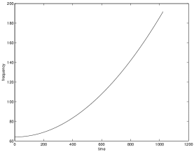
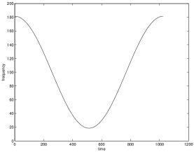
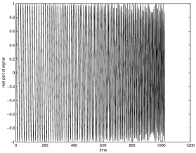
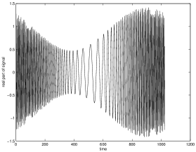
Note that because of the factor $N$ in the exponential (6.2), we are not sampling the same signal at increasingly fine rates. Instead, the instantaneous frequency of $S$ is actually changing with $N$ and is equal to $N\varphi^{\prime}(t)$ so that the signal may oscillate at nearly the sampling rate no matter what $N$ is. Figures (4) and (5) show the rescaled instantaneous frequency, $\varphi^{\prime}(t)$ and the real part of the signals under study for $N=1024$.

(a)		(b)

Figure 4: Instantaneous frequency $\varphi^{\prime}(t)$ of the chirps under study. (a) Cubic phase chirp. (b) Cosine phase chirp.

(a)		(b)

Figure 5: Real part $A(i/N)\cos(N\varphi(i/N))$, $i=0,\ldots,N-1$ of the of the chirps under study. (a) Cubic phase chirp. (b) Cosine phase chirp. The cosine phase chirp has a slowly varying amplitude. Note that the instantaneous frequency depends on the sample size $N$.

For detection, we use the BP test statistic introduced in Section 3.1 with $\{1,2,4,8,16\}$ as our discrete set of path lengths. We estimated the distribution of the minimum $P$-value under the null hypothesis via Monte Carlo simulations, and selected a detection threshold giving a probability of false detection (Type I error) equal to $5\%$ (.05 significance level).

• For each signal length, we randomly sampled about 10,000 realizations of white noise to compute the 5% detection level (the quantile of the minimum $P$-value distribution).

• For each signal length, each signal and each SNR, we sampled the data model about 1,000 times in order to compute detection rates, or equivalently the so-called power curves.

In these simulations, we only considered chirplets with positive frequencies and for the larger signal sizes, $N=2048,4096$, we restricted ourselves to discrete frequencies on the interval $\{0,\ldots,N/4-1\}$ to save computational time. In all cases the slope parameters $a_{\mu}$ of the chirplets (see equation (2.1)) ranged from $-\pi N$ to $\pi N$ with a discretization at scale $2^{-j}$ of the form $a_{\mu}=2\pi N(-1/2+k\cdot m2^{j-J})$ where $J=\log_{2}N$; $m=1$, $k\in\{0,\dots,2^{J-j}\}$ for signal lengths $N=512,1024,2048$ and $m=4$, $k\in\{0,\dots,2^{J-j-2}\}$ for $N=4096$. This ensures that any endpoint of a dyadic interval is an integer multiple of $2\pi$.

The scales considered ranged from the coarsest $2^{0}$ to $2^{-s}$ with $s=6$ for $N=512,1024$, $s=5$ for $N=2048$ and $s=4$ for $N=4096$ (the motivation is again speed). In practice, these parameters would depend upon the application and would need to be selected with care. Tables 1 and 2 show the correlation between the waveforms and the best chirplet path with a fixed length. Although we use a coarser discretization and fewer scales when $N=4096$, the correlation is still very high, at least for path lengths 8 and 16. Table 3 shows the correlations between the cosine phase chirp and chirplets with adapted amplitudes. As expected, the correlation increases.

signal length $N$	$\ell=1$	$\ell=2$	$\ell=4$	$\ell=8$	$\ell=16$
512	0.0718	0.4318	0.7126	0.9905	0.9982
1024	0.0453	0.2408	0.5784	0.9814	0.9981
2048	0.0306	0.1643	0.5107	0.9469	0.9976
4096	0.0229	0.0953	0.4265	0.8158	0.9917

Table 1: Correlations between the cosine phase signal and the best chirplet path with fixed lengths $\ell\in\{1,2,4,8,16\}$.

signal length N	$\ell=1$	$\ell=2$	$\ell=4$	$\ell=8$	$\ell=16$
512	0.2382	0.8733	0.9903	0.9979	0.9999
1024	0.1498	0.6575	0.9883	0.9985	0.9997
2048	0.0932	0.3836	0.9671	0.9976	0.9995
4096	0.0590	0.2373	0.8734	0.9903	0.9971

Table 2: Correlations between the cubic phase signal and the best chirplet path with fixed lengths $\ell\in\{1,2,4,8,16\}$.

$d$ : degree of polynomials	$\ell=1$	$\ell=2$	$\ell=4$	$\ell=8$	$\ell=16$
$[2,1,1,1,1,1]$	0.1481	0.2852	0.5699	0.9612	0.9995
$[2,2,2,1,1,1]$	0.1481	0.3337	0.5999	0.9612	0.9995
$[2,2,2,2,2,2]$	0.1481	0.3337	0.6122	0.9823	0.9999

Table 3: Correlations between the cosine phase signal and the best chirplet path with fixed lengths $\ell\in\{1,2,4,8,16\}$ (chirplets with varying amplitude). $N=2048$. The first column indicates the degree of the polynomial used to fit the amplitude. The entry $d_{j}$ in $d=[d_{0},d_{1},\ldots,d_{5}]$ is the degree of the polynomial at scale $2^{-j}$.

6.2 Results from simulations

To measure the performance of the BP statistic, we fix the probability of Type I error at $5\%$ and estimate the detection rate, the probability of detecting a signal when there is signal. We compute such detection curves for various SNRs (6.1). To limit the number of computations we focus on a small set of signal levels around the transition between a poor and a nearly perfect detection.

Figures 6 and 7 present results of a simulation study and display the power curves for both chirps and for various sample sizes. Of course, as the sample size increases, so does the sensitivity of the detector (even though the signal is changing with the sample size). We also note that the detection of the cubic phase chirp is slightly better than that of the cosine phase chirp which was to be expected since the cubic phase chirp is slightly less complex. (Simulations where one also adapts the amplitude give similar results.)

Figure 6: Detection rates of the cubic phase chirp with the BP method. The type I error is fixed at 5%.

Figure 7: Detection rates of the cosine phase chirp with the BP method. The type I error is fixed at 5%.

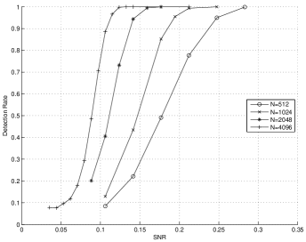
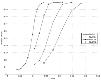
Consider the cosine phase chirp with time-varying amplitude and a sample size $N$ equal to $4,096$. Then the SNR for a detection level in the $95\%$ range is about .12. This means that one can reliably detect an unknown chirp of about this complexity when the amplitude of the noise is about 8 times that of the unknown signal.

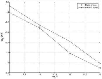
It is interesting to study the performance gain when we increase the signal length. Fix a detection rate at 95% and plot the SNR that achieves this rate against the sample size $N$. Figure 8 shows the base-2 logarithm of the estimated SNR (using a simple linear interpolation of the power curves) versus the logarithm of the sample size. The points roughly lie on a line with slope -0.4; as we double the signal length from $N$ to $2N$, the SNR required to achieve a 95% detection rate is about $2^{-0.4}\approx 0.76$ times that required to achieve the same detection rate for the signal length $N$. In a parametric setting, we would asymptotically expect a slope of -0.5. The fact that the slope is slightly higher than this is typical of nonparametric detection problems which deal with far richer classes of unknown signals [16].

Figure 8: Log-log (base-2) plot of the estimated SNR (for both chirps) at the $95\%$ detection rate versus signal length $N$. Again the Type I error is fixed at $5\%$. In both cases, the slope is approximately equal to -0.4.

6.2.1 Comparison with the detection a known signal

In order to see how sensitive our test statistic really is, it might be instructive to compare the detection rates with those one would achieve if one had full knowledge about the unknown signal. We then consider a simple alternative

$$H_{1}:y=\alpha S_{0}+z,$$

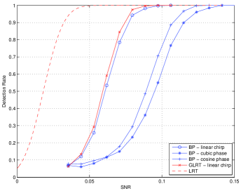
where the signal is known. That is, if there is signal, we know exactly how it looks like. The standard likelihood ratio test (LRT) gives the optimal test in terms of maximizing the power of detection at a given confidence level. A simple calculation shows that the 5% level, the power function of the LRT is equal to $\Phi(1.65-\text{SNR}\sqrt{2N})$ where $\Phi$ is the cumulative distribution of a standard normal. Figure 10 shows this power curve together with those obtained via the BP test for a sample size $N=4096$. The horizontal gap between curves indicates the ratio between SNRs to achieve the same detection rate. Consider a detection level equal to about $95\%$. Our plot shows that one can detect a completely unknown signal via the BP statistic with the same power than that one would get by knowing the signal beforehand provided that the amplitude is about 3 times as large. Note that this ratio is small and may be thought as the price one has to pay for not knowing in advance what it is.

6.2.2 Detection of a monochromatic sinusoid

To appreciate the performance of the BP statistic, it might be a good idea to study a more subtle problem. Suppose that the unknown signal is a monofrequency sinusoid. If there is signal, we know it is of the form $S(t)=e^{i\omega t+\phi}$, where the frequency $\omega$ and the phase shifts are unknown. Consider the simpler case where for a discrete signal of length $N$, $\omega\in\{0,\ldots,N-1\}$ is one of the $N$ Nyquist frequencies. Letting $y^{0}$ and $y^{1}$ be the real and imaginary parts of the data $y$, the GLRT would maximize

$$\sum_{0\leq t\leq N-1}y^{0}_{t}\cos(2\pi kt/N+\phi)+y^{1}_{t}\sin(2\pi kt/N+\phi),$$

over $k=0,1,\ldots,N-1$ and $\phi\in[0,2\pi]$. One can take the maximum over $\phi$ and check that the GLRT is equivalent to maximizing

$$\left|\sum_{0\leq t\leq N-1}y_{t}e^{-i2\pi kt/N}\right|$$

over $k$. Thus, the GLRT has a simple structure. It simply computes the DFT of the data, and compares the maximal entry of the response with a threshold. (Note the resemblance of this problem with the famous problem of testing whether the mean of Gaussian vector is zero versus an alternative which says that one of its component is nonzero.)

We could also make the problem a tiny bit harder by selecting the frequency arbitrarily, i.e. not necessarily a multiple of $2\pi$ but anything in the range $[0,2\pi N]$. In this case, the method described above would be a little less efficient since the energy of the signal would not be concentrated in a single frequency mode but spill over neighboring frequencies. The GLRT would ask to correlate the data with the larger collection of monofrequency signals which in practice we could approximately achieve by oversampling the DFT (e.g. we could select a finer frequency discretization so that the correlation between the unknown monochromatic signal we wish to detect and the closest test signal exceeds a fixed tolerance, e.g. .90 or .99).

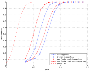
We compare the detection rate curve for detecting (i) a monochromatic sinusoid with integer frequency and (ii) a monochromatic sinusoid with arbitrary frequency using the maximum absolute DFT coefficient on one hand, and the BP test on the other hand. The signals in (i) and (ii) are equispaced samples from $S_{1}(t)=e^{\mathrm{i}2\pi\frac{N}{8}t}$ and $S_{2}(t)=e^{\mathrm{i}2\pi(\frac{N}{8}+\frac{1}{2})t}$. The signal length $N$ is equal to 4096. Figure 9 displays the detection rates. Consider the 95% detection rate. Then for (i) the SNR for the BP test is about $20\%$ higher than that for the GLRT. In (ii) the SNR is only $8\%$ higher. Also, at this detection level, the ratio between the SNRs for the cosine phase chirp and the monofrequency is about 1.75. These results show that ‘the price we pay’ for being adaptive and having the ability to detect a rich class of chirping signals is low.

Figure 9: Comparison of the BP and GLRT (based on the maximum modulus of the Fourier coefficients) for monochromatic sinusoids. The type I error is set at $5\%$

6.2.3 Detection of a linear chirp

To study ‘the price of adaptivity,’ we also consider the problem of detecting linear chirps. Suppose that the unknown signal are sampled values of a linear chirp of the form $S(t)=e^{i2\pi N\varphi(t)}$ where $\varphi(t)=at^{2}/2+bt+c$. Here, $N=4096$ and the coefficients $a,b,c$ are adjusted so that the unknown linear chirp is a complex multiple of a chirplet at the coarsest scale (the GLRT is then the BP test restricted to paths of length 1). In the simulations, we selected a chirp with $a=1/8$, $b=1/16$, and $c=0$ so that the instantaneous frequency $N\varphi^{\prime}(t)$ increased linearly from 256 to 768. Figure 10 displays the detection rates for the GLRT and the BP test with $\{1,2,4,8,16\}$ as path lengths. The detection rates for the BP test and the GLRT are almost the same; the ratio between the SNRs required to achieve a detection rate of about $95\%$ is about 1.05. This shows the good adaptivity properties of the BP test. For information, the plot also shows that one can detect a completely unknown signal via the BP statistic with the same power than that one would get for detecting a linear chirp via the GLRT provided that the amplitude is about 1.5 times as large.

Figure 10: Comparison of the BP and GLRT detection rates over a set of linear chirps. The type I error is set at $5\%$. Detection rates are plotted along with the detection rates for the cubic and cosine phase chirps.

6.3 Empirical adaptivity on a simulated gravitational wave

Earlier, we argued that the GLRT or the method of matched filters would need to generate exponentially many waveforms to provide good correlations with the unknown signal of interest. The idea underlying the chirplet graph is that one can get very good correlations by considering a reasonably sized dictionary and considering correlations with templates along a path in the graph. Figure 11 shows the real part of a ‘mock’ gravitational waveform whose instantaneous frequency and amplitude increase roughly as a power law as in Section 1.2. The waveform is $S(t)=A(t)e^{\mathrm{i}\varphi(t)}$ where the phase is

$$\varphi(t)=a_{0}(t_{c}-t)^{5/8}+a_{1}(t_{c}-t)^{3/8}+a_{2}(t_{c}-t)^{1/4}+a_{3}(t_{c}-t)^{1/8},$$

and the amplitude is given by $A(t)=[\varphi^{\prime}(t)]^{2/3}$ (see Figure 11).

Figure 11: Real part of a simulated gravitational wave

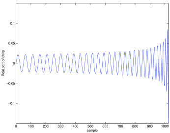
The coefficients $a_{0},\ldots,a_{3}$ where chosen from the post-Newtonian approximation for a binary inspiral as described in [4, 3]. The coefficient $t_{c}$ is the time of coalescence. The masses of the two bodies where both chosen to be equal to $14$ solar masses and the sampling rate was $2048$ Hz. We studied the last 1024 samples of the waveform.

As seen in Figure 12, the correlation with the noiseless waveform is equal to .95 with just 4 chirplets (with linear time-varying amplitudes) and .99 with just 5 chirplets. So we would not gain much (if anything at all) by computing inner products with exponentially many waveforms.

Figure 12: Chirplet paths returned by the BP test for path sizes equal to 1, 2, 3, 4, and 5 (the chirplets are adapted to have an amplitude varying linearly with time). The signal is a simulated gravitational wave. The cost here is simply the correlation between the waveform and the best chirplet path so that a value of 1 indicates a perfect match. The horizontal and vertical axes indicate time and frequency. The thin line is the ‘true’ instantaneous frequency of the waveform. The thick line is the value of the instantaneous frequency along the path.

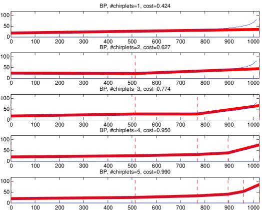
Another interesting aspect is that the best chirplet path automatically adapts to the unknown local complexity of the signal; it uses short templates whenever required and longer templates when the signal exhibits some coherence over longer periods of time. Here, the path is refined where the instantaneous frequency starts to rise, which occurs near the end of the period under study.

7 Discussion

We have presented a novel and flexible methodology for detecting nonstationary oscillatory signals. The approach chains together empirical correlations as to form meaningful signals which may exhibit very large correlations with the unknown signal we wish to detect. Our experiments show that our algorithms are very sensitive over very broad classes of signals. In this section, we discuss further directions and connections with the work of others.

7.1 Connection with other works

While working on this project [9] and writing this paper, we became aware of the recent and independent work of Chassande-Mottin and Pai which is similar in spirit to ours [12]. In this paper, the authors also search for a chirplet chain in a graph. Despite this similitude, our approach is distinct in several aspects. First, whereas Chassande-Mottin and Pai use chirplets at a single scale, we use a multiscale dictionary which provides high flexibility and adaptivity to the unknown structure of the signal (see Section 3.2); the last example in Section 6 also clearly demonstrates the promise of the multiscale approach for the practical detection of gravitational waves. Consequently our detection strategy based on the multiple comparison between test statistics with varying complexities is of course very different. Second, while we find the best path by dynamic programming, the best chirplet chain in [12] is not the solution to a tractable optimization problem since the statistic which needs to be maximized over a set of chirplet paths is not additive. Therefore the authors need to resort to a series of approximations involving time-frequency distributions such as the WVD to obtain an approximate solution. This makes our approach also different and more general since the methodology proposed in this paper may be applied in setups which have nothing to do with chirplets and chirp detection.

Finally, the aforementioned reference does not address the problem of detecting chirps with a time varying amplitude, and also assumes that the noise in the data is white or has been ‘whitened’ in some fashion (the detection method in [12] requires white noise). In contrast, the statistics in this paper have a natural interpretation in terms of likelihood ratios, and can be adapted effortlessly to more sophisticated setups in which the noise may be colored and in which the amplitude may also be rapidly varying and so on. Only the chirplet costs need to be changed while other algorithms remain the same.

7.2 Future directions

It would be of interest to develop a statistical theory of chirp detection and study whether or not our ideas are provably optimal in a decision theoretic sense. This would require the development of a meaningful model of chirps and show that for elements taken from this model, our methodology nearly obeys the same asymptotic performance than the minimax test or the Bayes test, should we take the Bayesian point of view to model our prior knowledge about chirps. We have investigated these issues and made progress on these problems. The tools required here seem rather different than those traditionally used in the mathematical theory of nonparametric detection [16]. We postpone our findings to a separate report.

There are several extensions to this work which seem worth investigating. First, we assumed implicitly that the chirp is present at all times. A more realistic model would need to include the possibility of chirps with a beginning and an end; i.e. we could only hear a chirp during a time interval which is shorter than that during which data is acquired. A more general strategy would then attempt to detect stretches of data which are not likely to be just noise. To isolate such candidate intervals, the dyadic thinking ideas of Castro et. al. [6] which consist of finding promising dyadic intervals and extending these promising intervals seem especially well suited. Another important extension would consider detection problems in which not one but several chirps may be present at once, i.e. the time frequency portrait of the data may include more than one spectral line.

Our main motivation for this work is the detection of gravitational waves. While this paper developed a new methodology for this problem, we did not go as far as testing these ideas on real data. We are now working on problems posed by real data (e.g. power line noise, transient events, nonstationarity etc.) and plan to report on our progress in a future publication. Of special interest is how one should subsample the chirplet transform and set the connectivities in the graph to build sensitive detectors which can deal with large scale data streams while still demanding manageable computing resources.

7.3 ChirpLab

The software package ChirpLab implements the algorithms proposed in this paper, and is available at http://www.acm.caltech.edu/$\sim$emmanuel/chirplet.html. It contains a Matlab implementation of the chirplet transforms and of all the optimization problems. Several Matlab scripts and a tutorial are provided to demonstrate how to use this software.

8 Appendix

8.1 Real-valued signals

In our simulations, we considered the detection of complex-valued chirps and we now rapidly discuss ways to extend the methodology to real valued data where the signal is of the form $S(t)=A(t)\cos(\lambda\varphi(t))$ with unknown phase and amplitude. Again, the idea is to build a family of real-valued chirplets which exhibit good local correlations with the signal. To do this, we could consider chirplets with quadratic phase $a_{\mu}t^{2}/2+b_{\mu}t+c_{\mu}$ and build a graph in which connectivities impose regularity assumptions on the phase function. The downside with this approach is that for each chirplet, one would need to introduce the extra phase-shift parameter $c_{\mu}$, which would increase the size of the dictionary and of the graph. This is not desirable.

A much better strategy is as follows: we parameterize chirplets in the same way with $v=(I,\mu)$ where $I$ is the time support of a chirplet and $a_{\mu}t+b_{\mu}$ is the instantaneous frequency, and define the chirplet cost by

$$C(v):=\max_{c}\frac{\left|\sum_{t\in I}y_{t}\cos(a_{\mu}t^{2}/2+b_{\mu}t+c)\right|^{2}}{\sum_{t\in I}\cos^{2}(a_{\mu}t^{2}/2+b_{\mu}t+c)}.$$ (8.1)

That is, we simply select the phase shift which maximizes the correlation (note that with complex data, the corresponding ratio $|\sum y_{t}\exp(\mathrm{i}(a_{\mu}t^{2}/2+b_{\mu}t+c))|^{2}/\sum|\exp(\mathrm{i}(a_{\mu}t^{2}/2+b_{\mu}t+c))|^{2}$ is, of course, independent of $c$). One can use simple trigonometric identities and write the numerator and denominator in (8.1) as

$$A^{2}\cos^{2}c-2AB\sin c\cos c+B^{2}\sin^{2}c,\quad C^{2}\cos^{2}c-2D\sin c\cos c+E^{2}\sin^{2}c,$$

where with $\varphi_{\mu}(t)=a_{\mu}t^{2}/2+b_{\mu}t$,

$$A+\mathrm{i}B=\sum y_{t}\,e^{\mathrm{i}\varphi_{\mu}(t)},\\$$

and

$$C^{2}=\sum\cos^{2}\varphi_{\mu}(t),\quad D=\sum\cos\varphi_{\mu}(t)\sin\varphi_{\mu}(t),\quad E^{2}=\sum\sin^{2}\varphi_{\mu}(t).$$

Note that $A+\mathrm{i}B$ is nothing else than the chirplet coefficient of the data and $C,D$, and $E$ can be computed off-line. There is an analytic formula for finding the value of $\cos c$ (or $\sin c$) that maximizes the ratio as a function of $A,B,C,D$, and $E$. This extends to the more sophisticated setups discussed in Section 5.

Finally, there are further approximations which one could use as well. Observe the expansion of the denominator in (8.1)

$$\sum_{t\in I}\cos^{2}(\varphi_{\mu}(t)+c)=|I|/2+1/2\,\sum_{t\in I}\cos(2\varphi_{\mu}(t)+2c),$$

where $|I|$ is here the number of time samples in $I$. Then for most chirplets (when the support contains a large number of oscillations), the second term in the right-hand side is negligible compared to the first. Assuming that the denominator is about equal to $|I|/2$ for all phase shifts $c$, we would then simply maximize the numerator in (8.1). A simple calculation shows that $e^{ic}=(A+\mathrm{i}B)/\sqrt{A^{2}+B^{2}}$ and

$$C(v)\approx 2\,\left|\sum_{t\in I}y_{t}e^{-\mathrm{i}(a_{\mu}t^{2}+b_{\mu}t)}/\sqrt{|I|}\right|^{2}.$$

(the “$\approx$” symbol indicates the approximation in the denominator). Hence, the real-valued cost is just about twice the usual complex-valued cost.

8.2 MCCTR algorithms

In this section, we briefly argue that one can compute the MCTTR introduced in Section 4.3 efficiently [2, 13]. Assume that $p^{\star}$ is the maximum value of $\sum_{i\in W}c(i,j)/|W|$ (with optimal solution $W^{\star}$) and that we have a lower bound $p_{0}$ on $p^{\star}$ (a trivial lower bound for the chirplet problem is $p_{0}=0$). Suppose that $W_{0}$ solves the SP problem with modified costs $c_{0}(i,j)=c(i,j)-p_{0}$. Then there are three possible cases, and we will rule one out:

1. $\sum_{W_{0}}c_{0}(i,j)<0$. Then $\sum_{W}c_{0}(i,j)\leq\sum_{W_{0}}c_{0}(i,j)<0$ for all paths $W$ and $\sum_{W^{\star}}c(i,j)/|W^{*}|<p_{0}\leq p^{\star}$. This is a contradiction and this case never comes up.

2. $\sum_{W_{0}}c_{0}(i,j)=0$. Then $\sum_{W}c_{0}(i,j)\leq\sum_{W_{0}}c_{0}(i,j)=0$ and, hence, $\sum_{W}c(i,j)/|W|\leq p_{0}$ for all paths $W$. We conclude that $p_{0}=p^{\star}$.

3. $\sum_{W_{0}}c_{0}(i,j)>0$. Then $\sum_{W_{0}}c(i,j)/|W_{0}|>p_{0}$ and we have a tighter lower bound on $p^{*}$. Take $p_{1}=\sum_{W_{0}}c(i,j)/|W_{0}|$ and repeat with the new costs $c_{1}(i,j)=c(i,j)-p_{1}$.

The MCTTR algorithm solves a sequence of SP problems, and visits a subset of the vertices on the boundary of the convex hull of the points $(|W|,C(W))$ until it finds the optimal trade-off. The number of vertices is of course bounded by the maximum possible length $\ell_{\max}$ of the path. In practice, the MCTTR converges after just a few iterations—between 4 and 6 in our simulations.

References

- [1] A. Abramovici, W. E. Althouse, R. W. P. Drever, Y. Gursel, S. Kawamura, F. J. Raab, D. Shoemaker, L. Sievers, R. E. Spero, and K. S. Thorne. LIGO - The Laser Interferometer Gravitational-Wave Observatory. Science, 256:325–333, April 1992.
- [2] R. K Ahuja, T. L. Magnanti, and J. B. Orlin. Network flows. Theory, algorithms and applications. Prentice-Hall, New-York, 1993.
- [3] B. Allen. Gravitational radiation analysis and simulation package (GRASP). Technical report, Department of Physics, University of Wisconsin, Milwaukee, P.O. Box 413, Milwaukee, WI 53201, 2000. Available at http://www.lsc-group.phys.uwm.edu/ballen/grasp-distribution/index.html.
- [4] W. G. Anderson and R. Balasubramanian. Time-frequency detection of gravitational waves. Physical Review D (Particles, Fields, Gravitation, and Cosmology), 60(10):102001, 1999.
- [5] E. Arias-Castro, E. J. Candès, and H. Helgason. Several examples of near optimal path detection from noisy data. 2006.
- [6] E. Arias-Castro, D. L. Donoho, and X. Huo. Near-optimal detection of geometric objects by fast multiscale methods. IEEE Trans. Inform. Theory, 51(7):2402–2425, 2005.
- [7] E. Arias-Castro, D. L. Donoho, and X. Huo. Adaptive multiscale detection of filamentary structures in a background of uniform random points. Ann. Statist., 34(1), 2006.
- [8] R. G. Baraniuk and D. L. Jones. Shear madness: New orthonormal bases and frames using chirp functions. IEEE Transactions on Signal Processing, 41(12):3543–3548, 1993.
- [9] E. J Candès, P. Charlton, and H. Helgason. Chirplets: recovery and detection of chirps. 2004. Presentation at the Institute of Pure and Applied Mathematics.
- [10] E. J Candès, P. Charlton, and H. Helgason. Detecting gravitational waves via chirplet path pursuit. 2006.
- [11] E. Chassande-Mottin and P. Flandrin. On the time-frequency detection of chirps. Appl. Comput. Harmon. Anal., 6(2):252–281, 1999.
- [12] E. Chassande-Mottin and A. Pai. Best chirplet chain: near-optimal detection of gravitational wave chirps. Phys. Rev. D, 73(4):042003 — 1–25, 2006.
- [13] G. B. Dantzig, W. O. Blattner, and M. R. Rao. Finding a cycle in a graph with minimum cost to time ratio with application to a ship routing problem. In Theory of Graphs (Internat. Sympos., Rome, 1966), pages 77–83. Gordon and Breach, New York, 1967.
- [14] D. L. Donoho and X. Huo. Beamlets and multiscale image analysis. In Multiscale and multiresolution methods, volume 20 of Lect. Notes Comput. Sci. Eng., pages 149–196. Springer, Berlin, 2002.
- [15] R. A. Helliwell. Whistlers and Related Atmospheric Phenomena. Stanford University Press, 1965.
- [16] Y. I. Ingster and I. A. Suslina. Nonparametric goodness-of-fit testing under Gaussian models, volume 169 of Lecture Notes in Statistics. Springer-Verlag, New York, 2003.
- [17] H. C. Joksch. The shortest route problem with constraints. J. Math. Anal. Appl., 14:191–197, 1966.
- [18] S. Mann and S. Haykin. The chirplet transform: Physical considerations. IEEE Transactions on Signal Processing, 43(11):2745–2761, 1995.
- [19] Y. Meyer. Oscillating patterns in image processing and nonlinear evolution equations, volume 22 of University Lecture Series. American Mathematical Society, Providence, RI, 2001. The fifteenth Dean Jacqueline B. Lewis memorial lectures.
- [20] M. Morvidone and B. Torresani. Time scale approach for chirp detection. Int. J. Wavelets Multiresolut. Inf. Process., 1(1):19–49, 2003.
- [21] B. J. Owen and B. S. Sathyaprakash. Matched filtering of gravitational waves from inspiraling compact binaries: Computational cost and template placement. Physical Review D (Particles, Fields, Gravitation, and Cosmology), 60(2):022002, 1999.
- [22] J. E. Reynolds III and S. A. Rommel. Biology of Marine Mammals. Smithsonian Institution Press, 1999.
- [23] A. Sha’ ashua and S. Ullman. The detection of globally salient structures using a locally connected network. In Proceedings of the Second International Conference on Computer Vision, pages 321–327, 1988.
- [24] J. Simmons. Echolocation in bats: signal processing of echoes for target range. Science, 171(974):925–928, 1971.
- [25] J. Simmons. The resolution of target range by echolocating bats. The Journal of the Acoustical Society of America, 54:157–173, 1973.
- [26] K. S. Thorne. Graviational radiation. In Stephen W. Hawking and Werner Israel, editors, 300 Years of Gravitation, pages 330–358. Cambridge University Press, Cambridge, England, 1987.
- [27] P. Westfall and S. Young. Resampling-based Multiple Testing: Examples and Methods for P-value Adjustment. Wiley, New York, 1993.