Rank deficiency and Tikhonov regularization in the inverse problem for gravitational-wave bursts

Abstract

Coherent techniques for searches of gravitational-wave bursts effectively combine data from several detectors, taking into account differences in their responses. The efforts are now focused on the maximum likelihood principle as the most natural way to combine data, which can also be used without prior knowledge of the signal. Recent studies however have shown that straightforward application of the maximum likelihood method to gravitational waves with unknown waveforms can lead to inconsistencies and unphysical results such as discontinuity in the residual functional, or divergence of the variance of the estimated waveforms for some locations in the sky. So far the solutions to these problems have been based on rather different physical arguments. Following these investigations, we now find that all these inconsistencies stem from rank deficiency of the underlying network response matrix. In this paper we show that the detection of gravitational-wave bursts with a network of interferometers belongs to the category of ill-posed problems. We then apply the method of Tikhonov regularization to resolve the rank deficiency and introduce a minimal regulator which yields a well-conditioned solution to the inverse problem for all locations on the sky.

Proc. of GWDAW-10 LIGO-P060005

1 Introduction

Efforts in searches for bursts with gravitational-wave detectors are now devoted to the development and testing of coherent data analysis techniques which do not require prior knowledge of the signal. Several such methods have been proposed in the past, beginning with the method of Gürsel and Tinto [1] which substantially predates all other techniques. The approach of Gürsel and Tinto is based upon explicit construction of a null data stream for two-polarization gravitational waves with completely arbitrary waveforms. Renewed interest in this method is motivated by the search for efficient vetoes of bursts of non-astrophysical origin [2]. Other methods which do not rely on the waveforms include coherent power filters [3] and cross-correlations of data from different detectors [4, 5, 6]. Recent studies are however converging on the maximum likelihood method as the most natural way to combine data from a network of gravitational wave detectors. It was shown by Flanagan and Hughes that the maximum likelihood inference can, in principle, be used without any knowledge of the anticipated signal [7]. This observation led to the development of a data analysis technique known as excess power [8]. Subsequent extensions of this approach included Karhunen-Loeve expansions [9] and non-parametric adaptive filters [10]. This groundwork helped building our confidence in the maximum likelihood method as a general framework for searches of gravitational-wave bursts with unknown waveforms. However, it was recently discovered that straightforward application of the maximum likelihood principle can lead to inconsistencies and unphysical results such as discontinuity in the residual functional called the two-detector paradox [11, 12], or unphysically large variations in the estimated signal-to-noise ratio [13]. The proposed solutions included constraints and penalty functions derived from various physical arguments [12, 13]. Continuing these investigations, we now consider the problem from a very general point of view. In this paper, we show that all these inconsistencies and paradoxes arise because the inverse problem for bursts belongs to the category of ill-posed discrete (matrix) problems. In particular, its underlying matrix of coefficients suffers from rank deficiency. It is then natural to look for a solution within the Tikhonov regularization approach [14] which is the general framework for solving ill-posed problems in mathematical physics.

2 The inverse problem for bursts

2.1 Network response

Consider a network of $m$ detectors located at different places on Earth. The response of the detectors to gravitational waves with two polarizations, $h_{+}$ and $h_{\times}$, is given by

$$\xi_{i}(t)=F_{i+}(\phi,\theta)\,h_{+}(t)+F_{i\times}(\phi,\theta)\,h_{\times}(t),$$ (1)

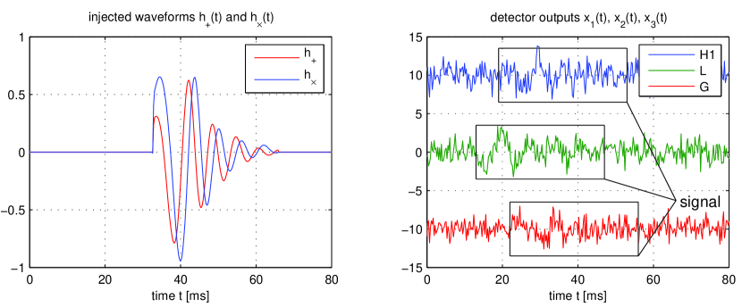
where $F_{i+}$ and $F_{i\times}$ are the antenna-pattern functions, and $\phi$ and $\theta$ are the spherical angles of the source in the sky. In general, the data from the network contains both signal and noise (see figure 1):

$$x_{i}(t)=\xi_{i}(t+\tau_{i})+\eta_{i}(t),$$ (2)

where the noise terms $\eta_{i}$ are assumed to be statistically independent among the detectors. The delays $\tau_{i}=\tau_{i}(\phi,\theta)$ depend on the source location and are calculated with respect to a common reference, usually taken at the center of Earth. After changing the variables: $t\rightarrow t-\tau_{i}$, we can write (1-2) in the matrix form:

$$x(t|\phi,\theta)=A(\phi,\theta)\,h(t)+\eta(t|\phi,\theta),$$ (3)

where $x$, $h$, and $\eta$ are column vectors and $A$ is $m\!\times\!2$ matrix,

$$A=\left[\begin{array}[]{cc}F_{1+}&F_{1\times}\\ \vdots&\vdots\\ F_{m+}&F_{m\times}\end{array}\right],$$ (4)

which will be called the network response matrix. The notation $x(t|\phi,\theta)$ implies that each component of the vector is shifted by its appropriate time delay:

$$x_{i}(t|\phi,\theta)=x_{i}[t-\tau_{i}(\phi,\theta)].$$ (5)

For simplicity, we will often omit $(\phi,\theta)$ and write (3) as

$$x(t)=A\,h(t)+\eta(t).$$ (6)

Also, it will be convenient to view the matrix $A$ as comprised of two vectors:

$$A=[\,{\mathbf{F}}_{+}\;{\mathbf{F}}_{\times}],$$ (7)

known as the range vectors of $A$ [15]. Examples of numerical calculations in this paper correspond to LIGO Hanford (H1 and H2), LIGO Livingston (L), VIRGO (V), and GEO-600 (G) detectors.

Figure 1: Simulated waveform injection. Left: a typical two-polarization waveform from numerical modeling of binary black hole coalescence [16]. Right: modeled detector outputs in H1-L-G network for a source located at $\phi=-60^{\circ}$ and $\theta=22^{\circ}$, with the matched-filter SNR [4] of 8, 12 and 7.

2.2 Moore-Penrose inverse

The inverse problem can be formulated as follows: given data from $m$ detectors $x_{i}(t)$ find the gravitational-wave amplitudes $h_{i}(t)$ and the source location in the sky $(\phi,\theta)$ by solving

$$A(\phi,\theta)\,h(t)=x(t|\phi,\theta),$$ (8)

in which the data is contaminated with noise. In general, the problem cannot be solved exactly, and one looks for an approximate solution by minimizing the functional

$$L[h]=\|x(t)-A\,h(t)\|^{2},$$ (9)

where $\|.\|$ stands for vector 2-norm:

$$\|x(t)\|^{2}=\sum_{i=1}^{m}\int_{0}^{T}x_{i}^{2}(t)\,dt,$$ (10)

defined over a suitable interval of observation $T$. The least squares (LSQ) functional $L[h]$ is usually derived within the maximum likelihood approach.

Variation of the functional $L[h]$ with respect to $h_{i}(t)$ yields the normal equations, which in the matrix form can be written as

$$M\,h(t)=A^{T}x(t),\qquad{\mathrm{where}}\qquad M=A^{T}A.$$ (11)

Then the solution is given by

$$h(t)=A^{\dagger}\,x(t),$$ (12)

where the $2\!\times\!m$ matrix

$$A^{\dagger}=M^{-1}A^{T}$$ (13)

is known as the Moore-Penrose inverse or pseudoinverse of matrix $A$ [17].

Consider now a situation when the data contains a signal,

$$x(t)=A(\phi_{s},\theta_{s})h_{s}(t)+\eta(t),$$ (14)

where $(\phi_{s},\theta_{s})$ represent the source position in the sky. Then the solution acquires a non-zero expectation value:

$$\langle h(t)\rangle=A^{\dagger}(\phi,\theta)A(\phi_{s},\theta_{s})\,h_{s}(t).$$ (15)

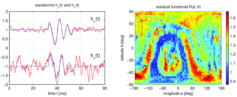
At the true location of the source $\langle h(t)\rangle=h_{s}(t)$, i.e. the solution given by the Moore-Penrose inverse yields an un-biased estimation of the gravitational-wave amplitudes. An example of a solution for $h(t)$ obtained from noisy data is shown in figure 2. Note that (12) provides the solution to the first part of the inverse problem: determination of $h(t)$. In the next section we describe the solution to the second part of the problem: determination of the source position on the sky $(\phi,\theta)$.

Introduction of the Moore-Penrose inverse allows us to define two complementary and orthogonal projector matrices:

$$P=AA^{\dagger},\qquad{\mathrm{and}}\qquad Q=I-AA^{\dagger}.$$ (16)

Note that $PA=A$ and $QA=0$ which means that $P$ projects onto the vector space of the range of matrix $A$ and $Q$ projects onto the null space of $A^{T}$, which is a subspace complementary to the range space.

Figure 2: Typical search results for the simulated waveform injection shown in figure 1. Left: injected (blue) and estimated (red) waveforms (after low-pass filtering). Right: sky map of the residual functional (17). The position of the source $(-60^{\circ},22^{\circ})$ is marked by $+$.

2.3 The residual functional

Substitution of the solution $h(t)$ (12) into $L[h]$ (9) yields the residual functional:

$$R=\|Qx\|^{2}=x^{T}Q\,x,$$ (17)

where we used the fact that $Q^{2}=Q$. This functional will be used to find the location of the source in the sky. We will now prove that the expectation value of $R(\phi,\theta)$ reaches minimum at the true location of the source. Assume that the data contains a signal (14), then the residual functional is given by

$$R=\|QA_{s}h_{s}\|^{2}+2\eta^{T}QA_{s}h_{s}+\eta^{T}Q\,\eta,$$ (18)

where $A_{s}\equiv A(\phi_{s},\theta_{s})$. The first term in (18) contains only deterministic quantities and therefore its expectation value is the same as its current value. The expectation value of the second term in vanishes because the signal does not correlate with the noise. Finally, the expectation value of the third term is given by

$$\langle\eta^{T}Q\,\eta\rangle = \sum_{i,j=1}^{m}Q_{ij}\int_{0}^{T}\langle\eta_{i}(t-\tau_{i})\eta_{j}(t-\tau_{j})\rangle\,dt$$ (19)

$$= \sum_{i,j=1}^{m}Q_{ij}\int_{0}^{T}\delta_{ij}\langle\eta_{i}^{2}(t)\rangle\,dt=\sigma^{2}\,\tr(Q),$$

where we assumed, for simplicity, that the noise in the detectors is Gaussian and its variance is $\sigma$. By transforming $Q$ to the diagonal form, one can show that $\tr(Q)=m\!-\!2$. Therefore,

$$\langle R(\phi,\theta)\rangle=\|QA_{s}h_{s}\|^{2}+\sigma^{2}\,(m-2).$$ (20)

At the true location of the source $QA_{s}=0$, and the function $\langle R(\phi,\theta)\rangle$ reaches its minimum. This concludes the solution to the second part of the inverse problem: determination of the source position (see figure 2). It is important to note that the function $\langle R(\phi,\theta)\rangle$ may have several minima on the sky of which only one corresponds to the true location of the source.

3 Examples of the inverse problem

The simplest types of the inverse problem occur in networks of 2 and 3 detectors.

3.1 $m=2$

In 2 dimensions the vectors ${\mathbf{F}}_{+}$ and ${\mathbf{F}}_{\times}$ span the entire vector space of columns of $A$, and there are no null vectors. In this case the inverse problem allows an exact solution

$$h=A^{-1}\,x,$$ (21)

for which the residual vanishes identically. It is worthwhile to obtain this result in a somewhat different way. Note that for $m=2$ the matrix $A$ is square and therefore $A^{\dagger}=A^{-1}$. Then

$$P=AA^{\dagger}=I,\qquad{\mathrm{and}}\qquad Q=0.$$ (22)

Consequently, $R(\phi,\theta)=0$ for every point on the sky, and no source localization is possible. In this case, every point in the sky, including the one which corresponds to the true source, can be viewed as a minimum of $\langle R(\phi,\theta)\rangle$.

3.2 $m=3$

In 3 dimensions the vectors ${\mathbf{F}}_{+}$ and ${\mathbf{F}}_{\times}$ span a 2-dimensional subspace of the vector space of columns of $A$. The complementary subspace, which is the space of null vectors, is therefore 1 dimensional, and is defined by one null vector, ${\mathbf{K}}$. The null condition $A^{T}K=0$ can be written in vector notation as

$${\mathbf{K}}\cdot{\mathbf{F}}_{+}={\mathbf{K}}\cdot{\mathbf{F}}_{\times}=0,$$ (23)

which implies that up to a multiplicative constant

$${\mathbf{K}}={\mathbf{F}}_{+}{\mathbf{\times}}\,{\mathbf{F}}_{\times}.$$ (24)

Knowing that $Q$ projects onto the null space, we obtain

$$Q_{ij}=\frac{K_{i}K_{j}}{|{\mathbf{K}}|^{2}},\qquad{\mathrm{and}}\qquad P_{ij}=\delta_{ij}-\frac{K_{i}K_{j}}{|{\mathbf{K}}|^{2}}.$$ (25)

Then from the definition (17) we find the residual functional,

$$R\equiv x^{T}Q\,x=\frac{\|{\mathbf{K}}\cdot{\mathbf{x}}\|^{2}}{|{\mathbf{K}}|^{2}},$$ (26)

which is the minimization functional of Gürsel and Tinto.

Next, we introduce two vectors to partition the Moore-Penrose inverse:

$$A^{\dagger}=[\,{\mathbf{H}}_{+}\;{\mathbf{H}}_{\times}]^{T},$$ (27)

so that the solution for $h$ (12) can be written as

$$h_{+}={\mathbf{H}}_{+}\cdot{\mathbf{x}},\qquad{\mathrm{and}}\qquad h_{\times}={\mathbf{H}}_{\times}\cdot{\mathbf{x}}.$$ (28)

It is easy to show that the partition vectors are given by

$${\mathbf{H}}_{+} = \frac{1}{|{\mathbf{K}}|^{2}}\;{\mathbf{F}}_{\times}\times{\mathbf{K}},$$ (29)

$${\mathbf{H}}_{\times} = \frac{-1}{|{\mathbf{K}}|^{2}}\;{\mathbf{F}}_{+}\times{\mathbf{K}}.$$ (30)

Indeed, from the definition of the Moore-Penrose inverse (13) we find that

$${\mathbf{H}}_{+} = [M^{-1}]_{11}\,{\mathbf{F}}_{+}+[M^{-1}]_{12}\,{\mathbf{F}}_{\times}$$ (31)

$$= (\det M)^{-1}\;\left[({\mathbf{F}}_{\times}\cdot{\mathbf{F}}_{\times})\,{\mathbf{F}}_{+}-({\mathbf{F}}_{+}\cdot{\mathbf{F}}_{\times})\,{\mathbf{F}}_{\times}\right]$$

$$= (\det M)^{-1}\;\;{\mathbf{F}}_{\times}\times({\mathbf{F}}_{+}\times{\mathbf{F}}_{\times}).$$

Combining this result with

$$\det M=|{\mathbf{K}}|^{2},$$ (32)

we obtain (29). Similarly, one can derive (30). Note that the solution for $h$, written in terms of ${\mathbf{H}}_{+}$ and ${\mathbf{H}}_{\times}$, is the waveform estimator of Gürsel and Tinto.

4 Difficulties with the LSQ minimization

Direct minimization of the LSQ functional encounters various difficulties, some of which are briefly described in this section.

4.1 Divergence of the expectation value of the solution

Consider the solution given by the Moore-Penrose inverse (12) as a function of sky position:

$$h(t)=M^{-1}(\phi,\theta)A^{T}(\phi,\theta)\,x(t).$$ (33)

As we have seen, on average, this solution correctly reproduces the waveform of the gravitational wave, provided that the estimated location of the source coincides with its true location. If, however, the estimated source location slightly deviates from the true location, the solution can be very different from the true waveform, especially near those places on the sky where the matrix $M$ becomes singular. Further discussion of the variations of the estimated waveforms and solutions based on the penalty functional can be found in [13].

4.2 Divergence of the variance of the solution

Consider now the error in estimation of the gravitational-wave amplitudes which comes from the presence of noise in the data:

$$\delta h(t)=A^{\dagger}(\phi,\theta)\eta(t).$$ (34)

Taking into account the fact that the noise in the detectors is uncorrelated, we obtain

$$\langle\delta h_{i}(t)\,\delta h_{j}(t^{\prime})\rangle = \sum_{k,l=1}^{m}[A^{\dagger}]_{ik}[A^{\dagger}]_{jl}\langle\eta_{k}(t)\,\eta_{l}(t^{\prime})\rangle$$ (35)

$$= \sigma^{2}[M^{-1}]_{ij}\delta(t-t^{\prime}).$$

Therefore, the variance of the solution,

$$\int_{0}^{T}\langle\delta h_{i}^{2}(t)\rangle\,dt=\sigma^{2}[M^{-1}]_{ii},$$ (36)

diverges as the estimated source location approaches those places in the sky where the matrix $M$ becomes singular. Solutions to this problem based on constraints applied to the waveforms can be found in [12].

4.3 Divergence of the residual functional

Finally, consider the residual functional (17). According to this definition the residual diverges if matrix $M$ becomes singular. This result becomes somewhat puzzling if we recall that in one particular case of singularity, namely when all detectors in the network are co-aligned, the residual in fact is well defined. Indeed, consider a network of $m$ co-aligned detectors. In this case it is not possible to solve for both $h_{+}$ and $h_{\times}$, and one can only solve for their linear combination: $\xi=F_{+}h_{+}+F_{\times}h_{\times}$. Then the LSQ functional takes the form [8]:

$$L[\xi]=\sum_{i=1}^{m}\|x_{i}(t)-\xi(t)\|^{2},$$ (37)

with an obvious solution: $\xi=\frac{1}{m}\sum_{i=1}^{m}x_{i}$. In this case, the projectors $P$ and $Q$ can be defined as

$$P_{ij}=\frac{1}{m},\qquad{\mathrm{and}}\qquad Q_{ij}=\delta_{ij}-\frac{1}{m}.$$ (38)

Consequently, the residual functional is given by

$$R\equiv x^{T}Q\,x=\frac{1}{m}\sum_{i,j=1}^{m}\int_{0}^{T}[x_{i}^{2}(t)-x_{i}(t)x_{j}(t)]\,dt.$$ (39)

Mathematically, this is an altogether different inverse problem, and there is no obvious reason why the solution of (37) must be related to the solution of the original inverse problem (9). However, our physical intuition tells us that the network of nearly aligned detectors must behave very similarly to a network in which the same detectors become fully aligned. Yet, the residual calculated for nearly aligned detectors (17) does not approach the one calculated for co-aligned detectors (39) in the limit when the detectors become perfectly aligned. This discontinuity of the residual functional becomes even more striking in two-detector networks for which $R=0$ (see section 3.1) for all detector orientations, no matter how close to perfect alignment they are. In this case the discrepancy was called the two-detector paradox [11, 12, 13].

5 Rank deficiency

All the above problems originate from rank deficiency of the network response matrix $A$. Recall that the nominal rank of $A$ is 2. The rank of $A$ drops to 1 if all the rows of $A$ become proportional to each other, which is known as full row degeneracy. Column degeneracy occurs when the two columns of matrix $A$ become proportional to each other. Note that full row degeneracy implies column degeneracy of $A$ and vice versa. In other words, either degeneracy results in collinearity of the range vectors:

$${\mathbf{F}}_{\times}=\beta\,{\mathbf{F}}_{+},$$ (40)

where $\beta$ is real. If this condition is satisfied, the rank of $A$ is 1. The simplest case of rank deficiency occurs when all detectors in the network are co-aligned and therefore all the rows of matrix $A$ are equal.

Figure 3: Condition number as a function of sky position (colormap in log scale). Left: LIGO-only network (H1-H2-L), Right: LIGO-GEO network (H1-H2-L-G). Note that close alignment of LIGO interferometers leads to very high condition number for some locations on the sky ($\gtrsim 10^{5}$), and the inclusion of GEO detector results in significant reduction of the condition number ($\gtrsim 10^{2}$).

In practice, we are seldom concerned with the exact collinearity of $\mathbf{F}_{+}$ and $\mathbf{F}_{\times}$ as the problem already occurs when these vectors are close to being collinear. This can be seen from the fact that

$$\det M=|{\mathbf{F}}_{+}|^{2}|{\mathbf{F}}_{\times}|^{2}-({\mathbf{F}}_{+}\cdot{\mathbf{F}}_{\times})^{2}\rightarrow 0,$$ (41)

as the two range vectors approach collinearity, making the Moore-Penrose inverse divergent. Quantitatively, the degree to which the inversion of $A$ becomes ill defined is described by the condition number [18]:

$${\mathbf{cond}}(A)=\|A\|\cdot\|A^{\dagger}\|,$$ (42)

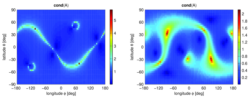
where $\|.\|$ stands for matrix 2-norm. Perfectly-invertible orthogonal matrices have condition number of 1. Large condition numbers indicate ill-defined inversion. Figure 3 shows condition numbers for two examples of detector networks. The locations in the sky with large condition number correspond to rank-deficient network response matrix.

6 Tikhonov regularization

Several techniques are available in applied mathematics to address rank deficiency of the coefficient matrix in the LSQ problem [18]. One of the most commonly used and best understood techniques is the Tikhonov regularization method [14]. The key idea in this method is to introduce a regularization functional (regulator) $\Omega[h(t)]$ with parameter $g>0$ such that the modified LSQ functional,

$$L_{g}[h]=\|x(t)-A\,h(t)\|^{2}+g\;\Omega[h],$$ (43)

no longer suffers from rank deficiency. Consider for example a quadratic regulator,

$$\Omega[h]\equiv h^{T}\Omega\,h=\sum_{i,j=1}^{m}\int_{0}^{T}\Omega_{ij}h_{i}(t)h_{j}(t)\,dt,$$ (44)

where $\Omega_{ij}$ is a symmetric 2$\times$2 matrix. Quadratic regulators preserve the linearity of the inverse problem and therefore have an advantage over other forms. Then the solution of the inverse problem becomes

$$h=M_{g}^{-1}A^{T}x,\qquad{\mathrm{where}}\qquad M_{g}=M+g\,\Omega.$$ (45)

Therefore, the regularized version of the Moore-Penrose inverse is

$$A_{g}^{\dagger}=M_{g}^{-1}A^{T},$$ (46)

which leads to the following generalization of matrices $P$ and $Q$:

$$P_{g}=AA_{g}^{\dagger},\qquad{\mathrm{and}}\qquad Q_{g}=I-AA_{g}^{\dagger}.$$ (47)

In general, these matrices no longer satisfy the property of projectors. However, the connection between the matrix $Q$ and the residual functional still holds. Indeed, substituting the solution (45) into the modified LSQ functional (43), we obtain

$$R_{g}=x^{T}Q_{g}\,x,$$ (48)

which is equivalent to (17) despite the presence of a regulator in $L_{g}[h]$.

The role of $\Omega$ is to render the inverse of $M_{g}$ well defined when $M$ is nearly singular. This resolves the problems associated with singularities of $M$, described in sections 4.1 and 4.2. Introduction of the regulator also solves the problem of discontinuity of the residual, described in section 4.3. Indeed, for $g\neq 0$ the residual $R_{g}$ is a continuous function of the detector alignment, and no divergence occurs in $R_{g}$ when the matrix $A$ becomes rank deficient (40). Furthermore, explicit calculations show that in this case

$$[P_{g}]_{ij}=\frac{\alpha}{\alpha+g\det\Omega}\;f_{i}f_{j},$$ (49)

where $\mathbf{f}$ is a unit vector along $\mathbf{F_{+}}$, and

$$\alpha=(\beta^{2}\Omega_{11}-2\beta\Omega_{12}+\Omega_{22})|\mathbf{F_{+}}|^{2}.$$ (50)

If the detectors in the network become co-aligned, $f_{i}=\frac{1}{\sqrt{m}}$ and therefore

$$[P_{g}]_{ij}=\frac{\alpha}{\alpha+g\det\Omega}\;\frac{1}{m}.$$ (51)

One can see from this expression that $P_{g}$ reduces to $P$ in (38), in the limit $g\rightarrow 0$, and consequently, $Q_{g}$ reduces to $Q$ in (38). Hence, the residual functional (48) reduces to that in (39).

7 Optimum condition regulator

As we have seen, the degree to which matrix $A$ becomes non-invertible, measured by the condition number, strongly depends on the sky location. It is therefore desirable to construct a regulator which is a function of sky position. Particularly useful will be regulators which adjust themselves to higher condition number, always guaranteeing well-defined inversion of $A$. Here we construct one example of such a regulator.

Figure 4: Condition number for LIGO-VIRGO network (H1-H2-L-V) as a function of sky position for different values of $g$ (colormap in log scale). Complete regularization takes place for $g=1$ (bottom-right) in which case the condition number is 1.

Consider matrix $M$ in the space of its eigenvectors:

$$\tilde{M}_{ij}=\left[\begin{array}[]{cc}\mu_{1}&0\\ 0&\mu_{2}\end{array}\right],$$ (52)

It is easy to show that its eigenvalues, $\mu_{1}$ and $\mu_{2}$, are always positive and one is always greater than the other, e.g. $\mu_{1}>\mu_{2}$. Since the purpose of a regulator is to prevent singularities which occur when $\mu_{1,2}\rightarrow 0$, it is sufficient to consider $\Omega$ which is diagonal in the space of eigenvectors of $M$:

$$\tilde{\Omega}_{ij}=\left[\begin{array}[]{cc}\omega_{1}&0\\ 0&\omega_{2}\end{array}\right],$$ (53)

where we assume that $\omega_{1,2}\geq 0$ so that $\Omega[h]$ is positive definite.

Figure 5: The residual functional (48), for LIGO-VIRGO network (H1-H2-L-V) with no regularization (left) and full regularization (right). The injected waveforms (figure 1) are amplified to produce the signals in detectors with the SNR of 8, 8, 12, and 10 for source location $(-60^{\circ},22^{\circ})$ (marked by $+$). Note a significant reduction in the degeneracy (blue area) introduced by the regulator.

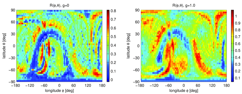
In most cases of interest only one of the eigenvalues, $\mu_{2}$, can be singular. If both eigenvalues vanish then $\mathrm{tr}(M)=0$. This would imply that $|\mathbf{F}_{+}|^{2}+|\mathbf{F}_{\times}|^{2}=0$, which, in turn, implies that all components of vectors $\mathbf{F}_{+}$ and $\mathbf{F}_{\times}$ vanish. In a given detector both antenna-pattern functions vanish only if the source is located in the plane of the detector, on the bisector of the detector arms, or on the normal to the bisector. Apart from the two Hanford interferometers, a general network of detectors does not have common arm bisectors or bisector normals, which is why both eigenvalues cannot vanish simultaneously.

A singularity in which one of the eigenvalues approaches zero whereas the other remains finite is known as a finite gap [18]. In this case, it is sufficient to regularize only the smallest eigenvalue $\mu_{2}$. We therefore limit ourselves to regulators in which $\omega_{1}=0$, and which are often called semi-norms in the space of solutions. Note that the parameter $g$ becomes redundant; it can be absorbed into $\omega_{2}$. Nevertheless, we retain $g$ so that we can control the strength of the regulator, and assume that the maximum value of $g$ is 1. We can now construct a regulator which makes the matrix $A$ fully invertible over the entire sky. Quantitatively, this means that for $g=1$

$$\mathbf{cond}(A)=\|A\|\cdot\|A_{g}^{\dagger}\|=1,$$ (54)

for all $\phi$ and $\theta$. Taking into account that

$$\|A\|=\sqrt{\mu_{1}},\qquad{\mathrm{and}}\qquad\|A_{g}^{\dagger}\|=\mathrm{max}\left(\frac{1}{\sqrt{\mu_{1}}},\frac{\sqrt{\mu_{2}}}{\mu_{2}+\omega_{2}}\right),$$ (55)

we find that the minimum value for such $\omega_{2}$ is given by

$$\omega_{2}^{*}=\sqrt{\mu_{1}\mu_{2}}-\mu_{2}.$$ (56)

In other words, any regulator of the semi-norm type in which $\omega_{2}>\omega_{2}^{*}$ yields the inversion of $A$ with condition number of 1.

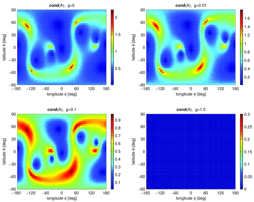
Figure 4 shows the improvement in the condition number for the LIGO-VIRGO network which results from this regularization. This will imply improvement in the accuracy of the solution for $h(t)$. Note that the introduction of the regularization also improves localization of the source on the sky, as shown in figure 5. Further analysis of the role of regularization will be given elsewhere. We conclude with the reminder that regularization, by its nature, introduces a bias and therefore the optimal approach must be a trade-off between the bias and the error due to noise.

8 Conclusion

We have shown that detection of gravitational-wave bursts of unknown waveforms is a linear inverse problem which becomes ill posed because of the rank deficiency of the underlying network response matrix. Following the general scheme of Tikhonov regularization, we introduced a semi-norm regulator in the space of solutions which guarantees full inversion of the network response matrix over the entire sky. The analysis presented here is general and applies to any network of interferometric gravitational-wave detectors. The problem of rank deficiency is particularly important from a practical point of view because the condition number for the LIGO-only network can be extremely high ($\gtrsim 10^{5}$) and regularization of the response matrix will play a crucial role in stabilizing the solution of the inverse problem. For networks in which LIGO detectors are accompanied by VIRGO or GEO interferometer the condition number is substantially better ($\gtrsim 10^{2}$) and yet still in need of regularization.

References

- [1] Gürsel Y and Tinto M 1989 Phys. Rev.D 40 3884
- [2] Wen L and Schutz B 2005 Class. Quantum Grav. 22 S1321
- [3] Sylvestre J 2003 Class. Quantum Grav. 20 S753
- [4] Cadonati L 2004 Class. Quantum Grav. 21 S1695
- [5] Cadonati L and Márka S 2005 Class. Quantum Grav. 22 S1159
- [6] Rakhmanov M and Klimenko S 2005 Class. Quantum Grav. 22 S1311
- [7] Flanagan É and Hughes S 1998 Phys. Rev.D 57 4566
- [8] Anderson W et al. 2001 Phys. Rev.D 63 042003
- [9] Viceré A 2002 Phys. Rev.D 66 062002
- [10] Chassande-Mottin E 2003 Phys. Rev.D 67 102001
- [11] Johnston W 2004 Detection strategies for a multi-interferometer triggered search Master’s thesis The University of Texas at Brownsville
- [12] Klimenko S et al. 2005 Phys. Rev.D 72 122002
- [13] Mohanty S et al. 2006 Class. Quantum Grav. 23 4799
- [14] Tikhonov A and Arsenin V 1977 Solutions of ill-posed problems (Washington, D.C.: V.H. Winston & Sons)
- [15] Golub G and Van Loan C 1989 Matrix Computations 2nd ed (Baltimore and London: The John Hopkins University Press)
- [16] Baker J et al. 2002 Phys. Rev.D 65 124012
- [17] Greville T 1959 SIAM Review 1 38
- [18] Hansen P 1998 Rank-deficient and discrete ill-posed problems (Philadelphia: SIAM)