On gravitational-wave spectroscopy of massive black holes with the space interferometer LISA

Abstract

Newly formed black holes are expected to emit characteristic radiation in the form of quasi-normal modes, called ringdown waves, with discrete frequencies. LISA should be able to detect the ringdown waves emitted by oscillating supermassive black holes throughout the observable Universe. We develop a multi-mode formalism, applicable to any interferometric detectors, for detecting ringdown signals, for estimating black hole parameters from those signals, and for testing the no-hair theorem of general relativity. Focusing on LISA, we use current models of its sensitivity to compute the expected signal-to-noise ratio for ringdown events, the relative parameter estimation accuracy, and the resolvability of different modes. We also discuss the extent to which uncertainties on physical parameters, such as the black hole spin and the energy emitted in each mode, will affect our ability to do black hole spectroscopy.

I Introduction

The Laser Interferometer Space Antenna (LISA) is being designed to observe gravitational waves in the low-frequency regime, between $10^{-5}$ and $10^{-1}$ Hz. A leading candidate source of detectable waves is the inspiral and merger of pairs of supermassive black holes (SMBHs). The signal should comprise three pieces: an inspiral waveform, a merger waveform and a ringdown waveform. The inspiral waveform, originating from that part of the decaying orbit leading up to the innermost stable orbit, has been analyzed using post-Newtonian theory and black-hole perturbation theory, and extensive studies of the detectability of this phase of the signal have been carried out (see eg. BBW ; BC and references therein). The nature of the merger waveform is largely unknown at present, and is the subject of work in numerical relativity.

The ringdown waveform originates from the distorted final black hole, and consists of a superposition of quasi-normal modes (QNMs). Each mode has a complex frequency, whose real part is the oscillation frequency and whose imaginary part is the inverse of the damping time, that is uniquely determined by the mass $M$ and angular momentum $J$ of the black hole. The amplitudes and phases of the various modes are determined by the specific process that formed the final hole.

The uniqueness of the modes’ frequencies and damping times is directly related to the “no hair” theorem of general relativistic black holes, and thus a reliable detection and accurate identification of QNMs could provide the “smoking gun” for black holes and an important test of general relativity in the strong-field regime dreyer .

In a pioneering analysis, Flanagan and Hughes (fh , henceforth FH) showed that, independently of uncertainties in the black hole spin and in the relative efficiency of radiation into various modes, the signal-to-noise ratio (SNR) for black hole ringdown could be comparable to that for binary inspiral. Consequently, both ringdown and inspiral radiation from SMBHs should be sufficiently strong relative to the proposed sensitivity of LISA that they may both be detectable with high SNR throughout the observable universe. With high SNR comes high accuracy, and hence the potential to measure ringdown QNMs and to test general relativity.

The FH analysis provided some insight into the issue of detectability of ringdown waves. However, to our knowledge, the problem of parameter estimation from black hole ringdown with LISA has not been discussed in depth in the literature to date. Most existing studies have referred specifically to high-frequency ringdown sources and Earth-based interferometers echeverria ; finn ; kaa ; creighton ; nakano ; tsunesada .

The main purpose of this paper is to discuss the measurability of ringdown QNM frequencies using LISA by carefully developing a framework for analyzing QNM radiation, and then applying the standard “Fisher matrix” formalism for parameter estimation finn . We will treat both single-mode and multi-mode cases.

From a mathematical point of view the excitation amplitude of QNMs is an ill-defined concept, because QNMs are not complete Beyer ; Beyer2 ; NollertPrice ; Nollert ; Szpak . Following leaver2 ; A94 ; Nils97 ; GA we will associate with each QNM an “excitation coefficient” that quantifies in a pragmatic (as opposed to rigorous) way the response of a black hole to perturbations with some given angular dependence. We will also define useful energy coefficients to characterize the energy deposited into various QNMs. Unfortunately, there is only sketchy information at present from numerical and perturbative simulations of distorted black holes, gravitational collapse or head-on collisions of two black holes as to what might be expected for the amplitudes, phases or energies of QNMs. It is clear that the QNM content of the waveform will depend strongly on the initial conditions and on the details of the distortion. In the absence of such information we will consider appropriate ranges of energy coefficients, and ranges of relative QNM amplitudes and phases as a way to assess the measurability of ringdown modes in some generality.

Although we will consider a range of SMBH masses from $10^{5}$ to $10^{8}\,M_{\odot}$, we note that, for masses smaller than about $10^{6}~{}M_{\odot}$, the damping time of the waves may be shorter than the light-travel time along the LISA arms, and as a consequence the number of observable oscillations will be so small that a Fisher matrix approach may not be fully reliable. We will also consider the full range of SMBH angular momenta, from zero to near extremal.

Figure 1: Value of $\epsilon_{\rm rd}$ required to detect the fundamental mode with $l=m=2$ (detection being defined by a SNR of $10$) at $D_{L}=3~{}$Gpc. For illustrative purposes here we pick the fundamental mode with $l=m=2$, but the dependence on $(n,l,m)$ is very weak. The three curves correspond to $j=0$ (solid), $j=0.8$ (dashed) and $j=0.98$ (dot-dashed), where $j=J^{2}/M=a/M$ is the dimensionless angular momentum parameter of the hole. The “pessimistic” prediction from numerical simulations of head-on collisions is $\epsilon_{\rm rd}=10^{-3}$ (as marked by the dashed horizontal line), so we should be able to see all equal-mass mergers with a final black hole mass larger than about $\sim 10^{5}~{}M_{\odot}$ (the vertical line is just a guide to the eye). The dip in the curves is a consequence of white-dwarf confusion noise in the LISA noise curve.

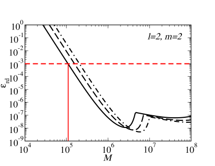
One of our conclusions is that the prospects for detection of ringdown radiation by LISA are quite encouraging. Figure 1 shows the value of the fraction of “ringdown energy” $\epsilon_{\rm rd}$ (defined as the fraction of the black hole mass radiated in ringdown gravitational waves) deposited in the fundamental “bar mode” with $l=m=2$ (assuming that mode dominates) that is required for the mode to be detectable by LISA with a SNR of 10 from a distance of 3 Gpc. Three values of the dimensionless angular momentum parameter $j\equiv J/M^{2}=a/M$ are shown: zero, 0.8 (an astrophysically interesting value), and 0.98. Recall that $0\leq j\leq 1$, spanning the range from Schwarzschild to extremal Kerr black holes. For SMBH masses between $10^{6}$ and $10^{7}\,M_{\odot}$, deposition energies as small as $10^{-7}$ of the mass should be detectable. We show that this conclusion is not strongly dependent on $(l,m)$, or on the overtone index $n$.

Figure 2: Errors (multiplied by the signal-to-noise ratio $\rho$) in measurements of different parameters for the fundamental $l=m=2$ mode as functions of the angular momentum parameter $j$. Solid (black) lines give $\rho\sigma_{j}$, dashed (red) lines $\rho\sigma_{M}/M$, dot-dashed (green) lines $\rho\sigma_{A}/A$, dot-dot-dashed (blue) lines $\rho\sigma_{\phi}$, where $\sigma_{k}$ denotes the estimated rms error for variable $k$, $M$ denotes the mass of the black hole, and $A$ and $\phi$ denote the amplitude and phase of the wave.

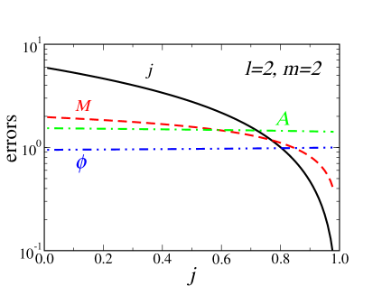
We also find that accurate measurements of SMBH mass and angular momentum may be possible. For detection of the fundamental $l=m=2$ bar mode, for example, Figure 2 shows the estimated error (multiplied by the SNR, $\rho$) in measuring the SMBH mass $M$, angular momentum parameter $j$, QNM amplitude $A$, and phase $\phi$ (see Sec. III for definitions). For example for an energy deposition of $10^{-4}M$ into the fundamental mode of a $10^{6}\,M_{\odot}$ SMBH with $j=0.8$ at 3 Gpc ($\rho\sim 200$), $M$ and $j$ could be measured to levels of a percent; if the energy deposition is only $10^{-6}$, they could still be measured to 10 percent. Generalizing to multi-mode detection (specifically to detection of two modes with a range of relative amplitudes), we find similar results.

Figure 3: “Critical” SNR $\rho_{\rm crit}$ required to resolve the fundamental mode ($n=0$) from the first overtone ($n^{\prime}=1$) with the same angular dependence ($l=l^{\prime}$, $m=m^{\prime}$). We assume the amplitude of the overtone is one tenth that of the fundamental mode. Solid lines refer to $m=l,..,1$ (bottom to top), the dotted line to $m=0$, and dashed lines to $m=-1,..,-l$ (bottom to top).

Figure 4: “Critical” SNR $\rho_{\rm both}$ required to resolve both the frequency and the damping time of the fundamental mode ($n=0$) from the first overtone ($n^{\prime}=1$) with the same angular dependence ($l=l^{\prime}$, $m=m^{\prime}$). We assume the amplitude of the overtone is one tenth that of the fundamental mode. Solid lines refer to $m=l,..,1$ (top to bottom), the dotted line to $m=0$, and dashed lines to $m=-1,..,-l$ (top to bottom, unless indicated). In the color versions, we used black for the modes with $l=|m|$, red for those with $0<|m|<l$ and blue for $m=0$. For $l=m$ the critical SNR grows monotonically as $j\to 1$.

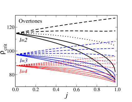
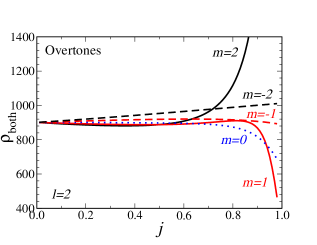
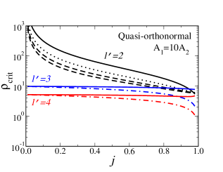
In order to test the no-hair theorem, it is necessary (though not sufficient) to resolve two QNMs dreyer ; roughly speaking, one mode is used to measure $M$ and $j$, the other to test consistency with the GR prediction. Using a simple extension of the Rayleigh criterion for resolving sinusoids, we estimate the SNR required to resolve the frequencies and/or the damping times of various pairs of modes, as a function of the angular momentum parameter $j$. For example, to resolve the fundamental $(n=0)$ mode for a given $(l,m)$ from the first overtone $(n=1)$ for the same $(l,m)$, the critical SNR required to resolve either frequency or damping time is shown in Fig. 3, while the SNR required to resolve both is shown in Fig. 4. These values assume that the amplitude of the overtone is $1/10$ that of the fundamental mode. Comparing Figs. 3 and 4 with Fig. 7 in Sec. III.2, we infer that tests of the no-hair theorem should be feasible, even under rather pessimistic assumptions about the ringdown efficiency $\epsilon_{rd}$, as long as the first overtone radiates a fraction $\sim 10^{-2}$ of the total ringdown energy. However, resolving both frequencies and damping times typically requires a SNR greater than about $10^{3}$. This is only possible under rather optimistic assumptions about the radiative efficiency, and it can be impossible if the dominant mode has $l=m=2$ and the black hole is rapidly spinning (solid black line in the left panel of Fig. 4). Requiring SNRs at least as large as $10^{2}$ implies that resolving QNMs will be impossible for redshifts larger than about 10.

The remainder of this paper provides details. In Sec. II we introduce our notation and formalism, and clarify some conceptual issues related to the QNM decomposition of gravitational waveforms. In Sec. III we compute the single-mode SNR assuming that only one mode dominates the ringdown. As a first step we update the FH analysis of LISA’s SNR for detection of single-mode waveforms. With respect to FH we use a better semianalytic approximation of the LISA noise curve, we consider different QNM frequencies, and we compare with the expected SNR for inspiral as computed in BBW . We explore the angular momentum dependence by considering black holes with $j\equiv a/M=0,~{}0.8,~{}0.98$, and confirm the FH expectation that angular momentum does not have a big effect on the SNR. Uncertainties in the ringdown efficiency $\epsilon_{\rm rd}$ have a larger impact, since $\rho\sim\sqrt{\epsilon_{\rm rd}}$. In Sec. IV we assess the accuracy of parameter estimation in single-mode situations, revisiting the analyses in echeverria ; finn ; kaa , and show that it is in general very good. A more detailed analysis shows that, for counterrotating ($m<0$) and axisymmetric ($m=0$) modes, rotation doesn’t necessarily help parameter estimation, and for some counterrotating modes the error can even blow up at “critical” values of the black hole angular momentum. Following preliminary remarks in Sec. V describing mathematical issues in and model predictions for multi-mode ringdowns, in Sec. VI we generalize to a two-mode analysis, computing the SNR and errors on parameter estimation. We find that it is computationally convenient to treat separately the case of waveforms in which the modes have different angular dependence ($l\neq l^{\prime}$ or $m\neq m^{\prime}$) and the case where the overtones have the same angular dependence as the fundamental mode. In Sec. VII we determine the minimum signal-to-noise ratio required to discriminate between different quasi-normal mode pairs. Conclusions and perspectives for future work are presented in Sec. VIII.

In the Appendices we collect various numerical results and technical calculations. Appendix A discusses the accuracy of a useful semianalytic approach to the calculation of the SNR (the $\delta$-function approximation, valid for ringdown signals with large quality factor). In Appendix B we present an explicit calculation of the Fisher matrix using different conventions and different numbers of free parameters in the ringdown waveform. Appendix C describes our semianalytical model of the LISA noise. Appendix D discusses a particular aspect of our criterion for resolving normal modes. Finally, Appendix E lists for reference the values of the complex frequencies and the angular separation constants of the spin-weighted spheroidal harmonics for selected normal modes, and also displays analytical fits of the QNM frequencies accurate within a few percent.

II Black hole ringing: preliminaries

II.1 Optimal mass range for ringdown detection by LISA

During the ringdown phase, perturbations of a Kerr black hole die away as exponentially damped sinusoids, whose frequencies and damping times are given by (complex) QNM frequencies kokkotas . We decompose the perturbations in spheroidal harmonics $S_{lm}(\iota,\beta)$ of “spin weight” 2 teukolsky ; berticardoso , where $l$ and $m$ are indices analogous to those for standard spherical harmonics, and $\iota$ and $\beta$ are angular variables such that the azimuthal, or $\beta$ dependence goes like $e^{{{\rm i}\beta}}$. For each ($l,m$) there is an infinity of resonant quasi-normal frequencies kokkotas , which control the intermediate time behavior of the signal. We label each of these frequencies by an overtone index $n$ such that the mode with $n=0$ has the longest damping time, followed by $n=1$ and so on. Thus, in the end QNM frequencies are parameterized by three numbers: $l\,,m$ and $n$. Now, the time dependence of the signal during ringdown is of the form $e^{{\rm i}\omega t}$, but since $\omega=\omega_{lmn}+{\rm i}/\tau_{lmn}$ is in general a complex number, we will follow the usual conventions and write this as $e^{-t/\tau_{lmn}}\sin\left(\omega_{lmn}t+\varphi_{lmn}\right)$, or $e^{-t/\tau_{lmn}}\cos\left(\omega_{lmn}t+\varphi_{lmn}\right)$, where $\omega_{lmn}=2\pi f_{lmn}$ is the mode’s real part and $\tau_{lmn}$ is the damping time of the oscillation. We will also define the quality factor of a QNM as

$$Q_{lmn}\equiv\pi f_{lmn}\tau_{lmn}=\omega_{lmn}\tau_{lmn}/2\,.$$ (1)

In our analysis of the detectability of ringdown radiation, we will assume that the signal lasts for at least one light-propagation time corresponding to the LISA arm length $L\simeq 5\cdot 10^{9}$ m, or $T_{\rm light}=L/c\simeq 16.68~{}{\rm s}$ (shorter-lived signals may require specialized detection techniques). This places a rough lower limit on the black hole masses that are relevant. To see this, we note that the fundamental mode of a Schwarzschild black hole corresponds to an axially symmetric ($m=0$), quadrupolar ($l=2$) perturbation with frequency

$$f_{200}=\pm 1.207\cdot 10^{-2}(10^{6}M_{\odot}/M)~{}{\rm Hz}\,,$$ (2)

and damping time

$$\tau_{200}=55.37(M/10^{6}M_{\odot})~{}{\rm s}\,.$$ (3)

Figure 5: Frequency $f_{lmn}$ (left) and quality factor $Q_{lmn}$ (right) for the fundamental modes with $l=2,~{}3,~{}4$ and different values of $m$. Solid lines refer to $m=l,..,1$ (from top to bottom), the dotted line to $m=0$, and dashed lines refer to $m=-1,..,-l$ (from top to bottom). Quality factors for the higher overtones are lower than the ones we display here.

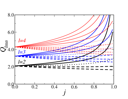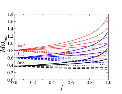
For rotating holes, the dimensionless frequencies ($M\omega_{lmn}$) and quality factors for the fundamental modes for $l=2,\,3,\,4$ are shown as a function of $j$ in Fig. 5. Although the quality factors and damping times for corotating ($m>0$) modes may be larger for rapidly rotating holes, the effects are not dramatic: for $j=0.80$ the damping time $\tau_{220}=65.18\left(M/10^{6}M_{\odot}\right)$ s, and for $j=0.98$ the damping time $\tau_{220}=127.7\left(M/10^{6}M_{\odot}\right)$ s. Accordingly we will restrict our attention to masses larger than $10^{6}$ or a few times $10^{5}M_{\odot}$.

We can also estimate an upper limit for masses to be considered by noting that LISA’s low frequency noise may provide a lower cutoff at $10^{-4}$ Hz. Equation (2) then gives a mass upper limit of around $10^{8}M_{\odot}$; if the LISA performance can be extended down to $10^{-5}$ Hz, then masses as large as $10^{9}M_{\odot}$ may be detectable. Again, these rough bounds are not terribly dependent on the black hole spin or the mode.

II.2 Quasinormal mode decomposition and polarization of the waveform

The plus and cross components of the gravitational waveform emitted by a perturbed Kerr black hole can be written in terms of the radial Teukolsky function $R_{lm\omega}$ as teukolsky

$$h_{+}+{\rm i}h_{\times}=-\frac{2}{r^{4}}\int_{-\infty}^{+\infty}\frac{d\omega}{\omega^{2}}e^{{\rm i}\omega t}\sum_{lm}S_{lm}\left(\iota,\beta\right)R_{lm\omega}(r)\,.$$ (4)

The radial Teukolsky function $R_{lm\omega}\sim r^{3}Z_{lm\omega}^{\rm out}e^{-{\rm i}\omega r}$ as $r\to\infty$, where $Z_{lm\omega}^{\rm out}$ is a complex amplitude NRezzolla .

We assume that the gravitational wave signal during the ringdown phase can be expressed as a linear superposition of exponentially decaying sinusoids. QNMs are known not to be a complete set, and thus such an expansion is not well defined mathematically. However numerical simulations of a variety of (perturbative and non-perturbative) dynamical processes involving black holes show that, at intermediate times, the response of a black hole is indeed well described by a linear superposition of damped exponentials. We defer further discussion of the meaning of the QNM expansion to Sec. V. For the time being, we just assume that we can write the gravitational waveform as a formal QNM expansion (rather than as a standard Fourier expansion in the real frequency $\omega$) of the Teukolsky function, so that we can replace Eq. (4) by

$$h_{+}+{\rm i}h_{\times}=\frac{1}{r}\sum_{lmn}e^{{\rm i}\omega_{lmn}t}e^{-t/\tau_{lmn}}S_{lmn}\left(\iota,\beta\right)Z_{lmn}^{\rm out}\,,$$ (5)

where $n$ denotes the overtone index and from here on the coordinate $t$ stands for the retarded time $t-r$. We write the complex wave amplitude $Z_{lmn}^{\rm out}$ in terms of a real amplitude ${\cal A}_{lmn}$ and a real phase $\phi_{lmn}$, and to follow the FH convention we factor out the black hole mass $M$: $Z_{lmn}^{\rm out}=M{\cal A}_{lmn}e^{{\rm i}\phi_{lmn}}$. In this way we get

$$h_{+}+{\rm i}h_{\times}=\frac{M}{r}\sum_{lmn}{\cal A}_{lmn}e^{{\rm i}(\omega_{lmn}t+\phi_{lmn})}e^{-t/\tau_{lmn}}S_{lmn}\,.$$ (6)

In this expansion the spheroidal functions $S_{lmn}=S_{lm}(a\omega_{lmn})$ are evaluated at the (complex) QNM frequencies, so they are complex numbers (henceforth we drop the $(\iota,\beta)$ angular dependence on the $S_{lmn}$).

Figure 6: Fundamental $l=2$ QNM frequencies of the Kerr black hole in the range $j\in[0,0.99]$. Solid (blue) lines correspond to $m=2$, dot-dashed (black) lines to $m=1$, dotted (red) lines to $m=0$, dashed (green) lines to $m=-1$, and short dashed (violet) lines to $m=-2$.

One frequently finds in the literature the astrophysically reasonable assumption that only the $l=m=2$ mode is present in the waveform. This viewpoint has two conceptual flaws.

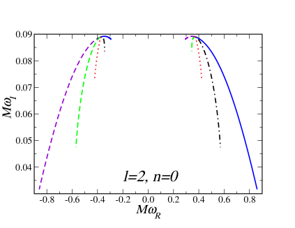
First, QNMs of Schwarzschild and Kerr black holes always come “in pairs”. In the Kerr case, for a given $(l,m)$ and a given value of $a=jM$ the eigenvalue problem admits two solutions: one with positive (real part of) the frequency, the other with negative real part of the frequency and different damping time. To illustrate this property, in Fig. 6 we show the fundamental Kerr QNM with $l=2$ and different values of $m$. Positive-$m$ frequencies are related to negative-$m$ frequencies by a simple symmetry property: one can easily see from the perturbation equations that to any QNM frequency characterized by $(l,m,n)$ there corresponds a QNM frequency characterized by $(l,-m,n)$ such that

$$-\omega_{lmn}=\omega_{l-mn}\,,\qquad 1/\tau_{lmn}=1/\tau_{l-mn}\,,\qquad A_{lmn}^{*}=A_{l-mn}\,,$$ (7)

(here $A_{lmn}$ is the angular separation constant, not to be confused with the mode amplitude ${\cal A}_{lmn}$). In this sense, any solution with positive $m$ is nothing but the “mirror image” of a solution with negative real part and negative $m$. For $m=0$ (and, of course, in the Schwarzschild case) the two “mirror solutions” are degenerate in modulus of the frequency and damping time. However, in general, a “mode with a given $(l,m)$” will always contain a superposition of two different damped exponentials. One of these exponentials could be invisible in the actual waveform because its damping time is shorter, or perhaps because it is less excited in the given physical situation, but formally one can never have anything like an isolated “$l=m=2$ frequency” with a positive real part. This excitation of both modes is actually observed in time-evolutions of perturbative fields in Kerr backgrounds krivan ; dorband .

Second, a single-mode expansion automatically restricts attention to circularly polarized gravitational waves; more generally one cannot specify the polarization state of the waveform by assuming that it is described by a single QNM frequency. This problem has been overlooked in all previous treatments of the gravitational radiation emitted during ringdown. This omission has no serious consequences for nonrotating holes, but it is conceptually inconsistent when $j\neq 0$. Consider, for example, the starting point of the analysis in FH. They assume that the waveform can be written as [Eq. (3.15) in FH]

$$h_{+}+{\rm i}h_{\times}=\frac{M{\cal A}_{lmn}}{r}e^{{\rm i}(\omega_{lmn}t+\phi_{lmn})}e^{-t/\tau_{lmn}}S_{lmn}\,,$$ (8)

with $l=m=2$. This is not a general assumption: it implies that the waves are circularly polarized.

On the contrary, the polarization of the ringdown waveform depends on the physical process generating the distortion of the black hole. In fact, most studies dealing with point particles in the vicinities of black holes show that the $h_{\times}$ component is extremely hard to excite nakamura . The only exception is provided by particles in circular motion, which do not resonantly excite QNMs anyway. To excite QNMs one needs an object passing through the potential barrier peak, for instance during the merger phase. In this case the motion is almost radial, so one can presumably lean on the point particle results and assume $h_{\times}\sim 0$ (see however lazarus ; AG for discussion of possible circular polarizations).

Accordingly, a consistent approach to ringdown waveforms begins with a general superposition of modes, including the “twin” modes with frequency $\omega^{\prime}_{lmn}=-\omega_{l-mn}$ and a different damping $\tau_{lmn}^{\prime}=\tau_{l-mn}$. Then, using the symmetry property (7) we can easily see that:

$$h_{+}+{\rm i}h_{\times} = \frac{M}{r}\sum_{lmn}\biggl{\{}{\cal A}_{lmn}e^{{\rm i}(\omega_{lmn}t+\phi_{lmn})}e^{-t/\tau_{lmn}}S_{lmn}+{\cal A}^{\prime}_{lmn}e^{{\rm i}(\omega^{\prime}_{lmn}t+\phi^{\prime}_{lmn})}e^{-t/\tau_{lmn}^{\prime}}S_{lmn}^{\prime}\biggr{\}}$$ (9)

$$= \frac{M}{r}\sum_{lmn}\biggl{\{}{\cal A}_{lmn}e^{{\rm i}(\omega_{lmn}t+\phi_{lmn})}e^{-t/\tau_{lmn}}S_{lmn}+{\cal A}^{\prime}_{lmn}e^{{\rm i}(-\omega_{l-mn}t+\phi^{\prime}_{lmn})}e^{-t/\tau_{l-mn}}S_{l-mn}^{*}\biggr{\}}$$

$$= \frac{M}{r}\sum_{lmn}\biggl{\{}{\cal A}_{lmn}e^{{\rm i}(\omega_{lmn}t+\phi_{lmn})}e^{-t/\tau_{lmn}}S_{lmn}+{\cal A}^{\prime}_{l-mn}e^{{\rm i}(-\omega_{lmn}t+\phi^{\prime}_{l-mn})}e^{-t/\tau_{lmn}}S_{lmn}^{*}\biggr{\}}$$

$$= \frac{M}{r}\sum_{lmn}\biggl{\{}{\cal A}_{lmn}e^{{\rm i}(\omega_{lmn}t+\phi_{lmn})}e^{-t/\tau_{lmn}}S_{lmn}+{\cal A}^{\prime}_{lmn}e^{{\rm i}(-\omega_{lmn}t+\phi^{\prime}_{lmn})}e^{-t/\tau_{lmn}}S_{lmn}^{*}\biggr{\}}\,.$$

In going from the second to the third line we relabeled $m\to-m$ in the second term, and in going from the third to the fourth line we changed the labeling of the (arbitrary) constants, replacing ${\cal A}^{\prime}_{l-mn}$ by ${\cal A}^{\prime}_{lmn}$ and $\phi^{\prime}_{l-mn}$ by $\phi^{\prime}_{lmn}$. So the general waveform depends on four arbitrary, real constants: ${\cal A}_{lmn}$, ${\cal A}^{\prime}_{lmn}$, $\phi_{lmn}$ and $\phi^{\prime}_{lmn}$ for each ($l,~{}m,~{}n$).

Thus it is clear that only by combining positive and negative values of $m$ can we require the waveform to have any given polarization state. In particular, if ${\cal A}_{lmn}e^{{\rm i}\phi_{lmn}}S_{lmn}={\cal A}^{\prime}_{lmn}e^{{\rm i}\phi^{\prime}_{lmn}}S_{lmn}^{*}$ the waveform becomes pure real (we have a “plus” state); if instead ${\cal A}_{lmn}e^{{\rm i}\phi_{lmn}}S_{lmn}=-{\cal A}^{\prime}_{lmn}e^{{\rm i}\phi^{\prime}_{lmn}}S_{lmn}^{*}$ it becomes pure imaginary (we have a “cross” state). In our single-mode analysis we will usually write the (real) plus and cross components measured at the detector as damped sinusoids, specifying arbitrarily their amplitude and relative phase. More rigorously, when we write the waveform as a damped sinusoid we really mean that we have performed a sum of the appropriate QNM components, as described above.

II.3 Including cosmological redshift

The general waveform (9) is written in the rest frame of the black hole, and thus all the quantities appearing there ($M\,,\,\omega_{lmn}$ and $\tau_{lmn}$) are measured in that frame. However, because of cosmological effects, in the detector’s frame all dimensionful quantities should be interpreted as redshifted. The prescription to include cosmological effects is very simple fh ; markovic : $r$ should be replaced by the luminosity distance $D_{L}(z)$, and all quantities with dimensions $[{\rm mass}]^{p}$ should enter the waveforms at the detector multiplied by the factor $(1+z)^{p}$. So, whenever the source is at cosmological distance, our $r$ should be replaced by $D_{L}(z)$, $M$ by the redshifted mass $(1+z)M^{0}$, $f_{lmn}$ by the redshifted frequency $f_{lmn}^{0}/(1+z)$, and $\tau_{lmn}$ by $(1+z)\tau_{lmn}^{0}$ (where all quantities marked by a superscript $0$ are measured in the source frame). In our numerical work, we use the values of cosmological parameters reported in cosmology .

III Signal-to-noise ratio for a single-mode waveform

III.1 Analytic Results

We begin by studying the SNR for detection of a single QNM. From Eq. (9), we can express the (real) waveform measured at the detector as a linear superposition of $h_{+}$ and $h_{\times}$, where, for the given mode $(l,~{}m,~{}n)$,

$$h_{+} = \frac{M}{r}\Re\left[{\cal A}^{+}_{lmn}e^{{\rm i}(\omega_{lmn}t+\phi_{lmn}^{+})}e^{-t/\tau_{lmn}}S_{lmn}(\iota,\beta)\right]\,,$$ (10a)

$$h_{\times} = \frac{M}{r}\Im\left[{\cal A}^{\times}_{lmn}e^{{\rm i}(\omega_{lmn}t+\phi_{lmn}^{\times})}e^{-t/\tau_{lmn}}S_{lmn}(\iota,\beta)\right]\,,$$ (10b)

where ${\cal A}^{+,\times}_{lmn}$ and $\phi_{lmn}^{+,\times}$ are real, and are related to the quantities ${\cal A}_{lmn}$, ${\cal A}^{\prime}_{lmn}$, $\phi_{lmn}$, and $\phi_{lmn}^{\prime}$ of Eq. (9) by ${\cal A}^{+,\times}_{lmn}e^{{\rm i}\phi_{lmn}^{+,\times}}={\cal A}_{lmn}e^{{\rm i}\phi_{lmn}}\pm{\cal A}^{\prime}_{lmn}e^{-{\rm i}\phi_{lmn}^{\prime}}$, where the $+(-)$ signs correspond to the $+(\times)$ polarizations, respectively. The waveform measured at a detector is given by

$$h=h_{+}F_{+}(\theta_{S},\phi_{S},\psi_{S})+h_{\times}F_{\times}(\theta_{S},\phi_{S},\psi_{S})\,,$$ (11)

where $F_{+,\times}$ are pattern functions that depend on the orientation of the detector and the direction of the source, given by

$$F_{+}(\theta_{S},\phi_{S},\psi_{S}) = \frac{1}{2}(1+\cos^{2}\theta_{S})\cos 2\phi_{S}\cos 2\psi_{S}-\cos\theta_{S}\sin 2\phi_{S}\sin 2\psi_{S}\;,$$ (12a)

$$F_{\times}(\theta_{S},\phi_{S},\psi_{S}) = \frac{1}{2}(1+\cos^{2}\theta_{S})\cos 2\phi_{S}\sin 2\psi_{S}+\cos\theta_{S}\sin 2\phi_{S}\cos 2\psi_{S}\;.$$ (12b)

To compute the SNR we will usually follow the prescription described in Appendix A of FH (henceforth the FH convention or FH doubling prescription) as follows: (1) Assume that the waveform for $t<0$ is identical to the waveform for $t>0$ except for the sign of $t/\tau_{lmn}$, i.e. that we replace the decay factor $e^{-t/\tau_{lmn}}$ with $e^{-|t|/\tau_{lmn}}$. (2) Compute the SNR using the standard expression,

$$\rho^{2}=4\int_{0}^{\infty}\frac{\tilde{h}^{*}(f)\tilde{h}(f)}{S_{h}(f)}df\,,$$ (13)

where $\tilde{h}(f)$ is the Fourier transform of the waveform, and $S_{h}(f)$ is the noise spectral density of the detector. (3) Divide by a correction factor of $\sqrt{2}$ in amplitude to compensate for the doubling-up in step (1).

In calculating the SNR, we will average over source directions and over detector and black-hole orientations, making use of the angle averages: $\langle F_{+}^{2}\rangle=\langle F_{\times}^{2}\rangle=1/5$, $\langle F_{+}F_{\times}\rangle=0$, and $\langle|S_{lmn}|^{2}\rangle=1/4\pi$. This simple averaging is feasible because the mode damping time is short compared to the orbital period of LISA.

Sometimes, for comparison, we will not follow the three steps we just described, but will calculate the Fourier transform of the waveform by integrating only over the range $t>0$. Since this was the method used by Echeverria echeverria and Finn finn , we will refer to this procedure as the Echeverria-Finn (EF) convention.

In the rest of this Section we will follow the FH prescription. The Fourier transform of the waveform can be computed using the elementary relation

$$\int_{-\infty}^{\infty}e^{{\rm i}\omega t}\left(e^{\pm{\rm i}\omega_{lmn}t-|t|/\tau_{lmn}}\right)dt=\frac{2/\tau_{lmn}}{(1/\tau_{lmn})^{2}+(\omega\pm\omega_{lmn})^{2}}\equiv 2b_{\pm}\,.$$ (14)

Then the Fourier transforms of the plus and cross components become:

$$\tilde{h}_{+} = \frac{M}{r}{\cal A}^{+}_{lmn}\left[e^{{\rm i}\phi_{lmn}^{+}}S_{lmn}b_{+}+e^{-{\rm i}\phi_{lmn}^{+}}S_{lmn}^{*}b_{-}\right]\,,$$ (15a)

$$\tilde{h}_{\times} = -{\rm i}\frac{M}{r}{\cal A}^{\times}_{lmn}\left[e^{{\rm i}\phi_{lmn}^{\times}}S_{lmn}b_{+}-e^{-{\rm i}\phi_{lmn}^{\times}}S_{lmn}^{*}b_{-}\right]\,.$$ (15b)

We can directly plug these Fourier transforms into the definition (13) of the SNR to get

$$\rho^{2}(\theta_{S},\phi_{S},\psi_{S},\iota,\beta) = 2\left(\frac{M}{r}\right)^{2}\int_{0}^{\infty}\frac{df}{S_{h}(f)}\times$$ (16)

$$\times\biggl{\{}\left(b_{+}^{2}+b_{-}^{2}\right)\left[{\cal A}^{+\,2}_{lmn}F_{+}^{2}+{\cal A}^{\times\,2}_{lmn}F_{\times}^{2}-2{\cal A}^{+}_{lmn}{\cal A}^{\times}_{lmn}F_{+}F_{\times}\sin(\phi_{lmn}^{+}-\phi_{lmn}^{\times})\right]|S_{lmn}|^{2}$$

$$+2b_{+}b_{-}\biggl{[}\Re\left[\left({\cal A}^{+\,2}_{lmn}F_{+}^{2}e^{2{\rm i}\phi_{lmn}^{+}}-{\cal A}^{\times\,2}_{lmn}F_{\times}^{2}e^{2{\rm i}\phi_{lmn}^{\times}}\right)S_{lmn}^{2}\right]$$

$$+2{\cal A}^{+}_{lmn}{\cal A}^{\times}_{lmn}F_{+}F_{\times}\Im\left(e^{{\rm i}(\phi_{lmn}^{+}+\phi_{lmn}^{\times})}S_{lmn}^{2}\right)\biggr{]}\biggr{\}}\,.$$

The terms proportional to $S_{lmn}^{2}$ cannot be angle-averaged analytically in the usual way, so to deal with this general expression one must perform a Monte Carlo simulation. Given randomly generated values of the angles we can compute numerically the spin-weighted spheroidal harmonics at the QNM frequencies, plug the harmonics into the integrals, and finally average the resulting SNRs. We leave this for future work.

However, especially for slowly-damped modes with $m\geq 0$, the imaginary part of $S_{lmn}$ is typically smaller than the real part:

$$S_{lmn}\simeq\Re(S_{lmn})\,,\qquad\,\Re(S_{lmn})\gg\Im(S_{lmn})\,.$$ (17)

We give a quantitative discussion of the validity of this approximation elsewhere berticardoso . We will henceforth assume that the $S_{lmn}$ are real, so that $S_{lmn}^{2}=|S_{lmn}^{2}|$, and we can complete the angle averaging analytically to obtain

$$\rho^{2} = \frac{1}{10\pi}\left(\frac{M}{r}\right)^{2}\int_{0}^{\infty}\frac{df}{S_{h}(f)}\times$$ (18)

$$\times\left\{\left(b_{+}^{2}+b_{-}^{2}\right)\left[{\cal A}^{+\,2}_{lmn}+{\cal A}^{\times\,2}_{lmn}\right]+2b_{+}b_{-}\left[{\cal A}^{+\,2}_{lmn}\cos(2\phi_{lmn}^{+})-{\cal A}^{\times\,2}_{lmn}\cos(2\phi_{lmn}^{\times})\right]\right\}\,.$$

We expect that the resulting SNR should be reasonably close to the true angle-averaged result as long as the imaginary part of the harmonics is not too large.

We make the further approximation that the damping time is sufficiently long that the frequency-dependent functions $b_{+}^{2}+b_{-}^{2}$ and $b_{+}b_{-}$ may be replaced by suitable $\delta$-functions, namely in the large $Q_{lmn}$ or large $\tau_{lmn}$ limit,

$$b_{+}^{2}+b_{-}^{2} \to \frac{\tau_{lmn}}{4}\left[\delta(f-f_{lmn})+\delta(f+f_{lmn})\right]\,,$$

$$b_{+}b_{-} \to \frac{\tau_{lmn}}{8}\frac{1}{1+4Q_{lmn}^{2}}\left[\delta(f-f_{lmn})+\delta(f+f_{lmn})\right]\,,$$ (19)

where the normalizations are obtained by integrating over positive frequencies only. This approximation is mathematically, though not physically equivalent to assuming that the noise density $S_{h}(f)$ is strictly constant. We then obtain the angle-averaged SNR,

$$\rho^{2}=\frac{Q_{lmn}}{40\pi^{2}f_{lmn}(1+4Q_{lmn}^{2})S_{h}(f_{lmn})} \times \left\{\left(\frac{M{\cal A}^{+}_{lmn}}{r}\right)^{2}\left[1+\cos(2\phi_{lmn}^{+})+4Q_{lmn}^{2}\right]\right.$$ (20)

$$+ \left.\left(\frac{M{\cal A}^{\times}_{lmn}}{r}\right)^{2}\left[1-\cos(2\phi_{lmn}^{\times})+4Q_{lmn}^{2}\right]\right\}\,.$$

For simplicity, FH also make an assumption about the relative amplitudes and phases of the waves, taking a pure cosine for the $+$-polarization ($\phi_{lmn}^{+}=0$), a pure sine for the $\times$-polarization ($\phi_{lmn}^{\times}=0$), and assuming ${\cal A}^{+}_{lmn}={\cal A}^{\times}_{lmn}={\cal A}_{lmn}$. With these assumptions, the SNR takes the form,

$$\rho_{\rm FH}^{2} = \left(\frac{M}{r}\right)^{2}\frac{{\cal A}^{2}_{lmn}}{80\pi^{5}\tau_{lmn}^{2}}\int_{0}^{\infty}\frac{df}{S_{h}(f)}\biggl{\{}\frac{1}{\left[(f+f_{lmn})^{2}+(2\pi\tau_{lmn})^{-2}\right]^{2}}+\frac{1}{\left[(f-f_{lmn})^{2}+(2\pi\tau_{lmn})^{-2}\right]^{2}}\biggr{\}}$$ (21a)

$$\simeq \left(\frac{M}{r}\right)^{2}\frac{Q_{lmn}{\cal A}^{2}_{lmn}}{20\pi^{2}f_{lmn}S_{h}(f_{lmn})}\,,$$ (21b)

where the second expression corresponds to the $\delta$-function limit.

It is now useful, following FH, to define an energy spectrum through the relation

$$\rho^{2}=\frac{2}{5\pi^{2}r^{2}}\int_{0}^{\infty}\frac{1}{f^{2}S_{h}(f)}\frac{dE}{df}df\,.$$ (22)

From Eq. (18), we obtain

$$\frac{dE}{df} = \frac{\pi M^{2}f^{2}}{4}\left\{\left(b_{+}^{2}+b_{-}^{2}\right)\left[{\cal A}^{+\,2}_{lmn}+{\cal A}^{\times\,2}_{lmn}\right]+2b_{+}b_{-}\left[{\cal A}^{+\,2}_{lmn}\cos(2\phi_{lmn}^{+})-{\cal A}^{\times\,2}_{lmn}\cos(2\phi_{lmn}^{\times})\right]\right\}\,.$$ (23)

We then define the “radiation efficiency” $\epsilon_{\rm rd}$, by

$$\epsilon_{\rm rd}\equiv\frac{E_{\rm GW}}{M}=\frac{1}{M}\int_{0}^{\infty}\frac{dE}{df}df\,.$$ (24)

Substituting Eq. (23) into (24) and integrating, and comparing the result with Eq. (20), we find a relation between SNR and radiation efficiency for a given mode, in the $\delta$-function or constant-noise limit,

$$\rho_{\rm FH}=\left(\frac{2}{5}\right)^{1/2}\left(\frac{1}{\pi f_{lmn}r}\right)\left(\frac{\epsilon_{\rm rd}M}{S_{h}(f_{lmn})}\right)^{1/2}\frac{2Q_{lmn}}{\sqrt{1+4Q_{lmn}^{2}}}\,.$$ (25)

independently of any condition on the relative amplitudes or phases.

With the FH choice of phases and amplitudes, the resulting energy spectrum is their formula (3.18):

$$\left(\frac{dE}{df}\right)_{\rm FH} = \frac{{\cal A}_{lmn}^{2}M^{2}f^{2}}{32\pi^{3}\tau_{lmn}^{2}}\biggl{\{}\frac{1}{\left[(f+f_{lmn})^{2}+(2\pi\tau_{lmn})^{-2}\right]^{2}}+\frac{1}{\left[(f-f_{lmn})^{2}+(2\pi\tau_{lmn})^{-2}\right]^{2}}\biggr{\}}$$ (26)

$$\simeq \frac{{\cal A}_{lmn}^{2}Q_{lmn}M^{2}f_{lmn}}{8}\delta(f-f_{lmn})\,.$$

where the second expression corresponds to the $\delta$-function limit. Integrating the FH energy spectrum (26) explicitly, we find that the amplitude is related to $\epsilon_{\rm rd}$ by

$${\cal A}_{lmn}=\sqrt{\frac{32Q_{lmn}\epsilon_{\rm rd}}{Mf_{lmn}(1+4Q_{lmn}^{2})}}\simeq\sqrt{\frac{8\epsilon_{\rm rd}}{MQ_{lmn}f_{lmn}}}\,,$$ (27)

where the second expression corresponds to the $\delta$-function limit.

Using our general spectrum (23) we can relate the polarization-phase dependent amplitude to an efficiency per polarization $\epsilon^{+,\times}_{\rm rd}$ by

$${\cal A}^{+,\times}_{lmn}=\sqrt{\frac{64Q_{lmn}\epsilon_{\rm rd}^{+,\times}}{Mf_{lmn}[1+4Q_{lmn}^{2}\pm\cos(2\phi_{lmn}^{+,\times})]}}\simeq\sqrt{\frac{16\epsilon_{\rm rd}^{+,\times}}{MQ_{lmn}f_{lmn}}}\,,$$ (28)

where the upper and lower signs refer to the $+$ and $\times$ polarizations, respectively, and where the last step again corresponds to the $\delta$-function limit.

The expressions used in this Section are valid for any interferometric detector. In all of our LISA calculations we take into account the fact that the LISA arms form an angle of 60 degrees; as a result, when integrating our results with the LISA noise curve, we must multiply all amplitudes by a geometrical correction factor $\sqrt{3}/2$, so that ${\cal A}^{LISA}_{+,\times}=\sqrt{3}/2\times{\cal A_{+,\times}}$.

We now combine the expression (25) with an analytic approximation for the LISA noise curve (here, for simplicity, we exclude white-dwarf confusion noise; see Appendix C) of the form

$$S_{h}^{\rm NSA}(f)=\left[9.18\times 10^{-52}\left(\frac{f}{1~{}{\rm Hz}}\right)^{-4}+1.59\times 10^{-41}+9.18\times 10^{-38}\left(\frac{f}{1~{}{\rm Hz}}\right)^{2}\right]~{}{\rm Hz}^{-1}\,.$$ (29)

Rescaling frequencies in terms of the dimensionless frequency ${\cal F}_{lmn}=M\omega_{lmn}$, and inserting redshift factors suitably, we obtain

$$\rho_{\rm FH}=\frac{5.1\times 10^{3}}{{\cal F}_{lmn}}\left(\frac{\epsilon_{\rm rd}}{0.03}\right)^{1/2}\left(\frac{(1+z)M}{10^{6}\,M_{\odot}}\right)^{3/2}\left(\frac{1\,{\rm Gpc}}{D_{L}(z)}\right)\left(\frac{S_{0}}{S_{h}(f_{lmn})}\right)^{1/2}\frac{2Q_{lmn}}{\sqrt{1+4Q_{lmn}^{2}}}\,,$$ (30)

where

$$\frac{S_{h}(f_{lmn})}{S_{0}}=\frac{5.4\times 10^{-5}}{{\cal F}_{lmn}^{4}}\left(\frac{(1+z)M}{10^{6}M_{\odot}}\right)^{4}+1+6.0\,{\cal F}_{lmn}^{2}\left(\frac{10^{6}M_{\odot}}{(1+z)M}\right)^{2}\,.$$ (31)

The dimensionless, mode-dependent quantities ${\cal F}_{lmn}$ and $Q_{lmn}$ are of order unity and vary relatively weakly from mode to mode; for low order modes they can be determined from the analytic fits discussed in Appendix E.

So far we have confined attention to the FH convention. If we follow the alternative EF convention of keeping the waveform only for $t>0$, and use the $\delta$-function limit, we get the SNR

$$\rho_{\rm EF}^{2}=\langle\rho^{2}\rangle=\frac{Q_{lmn}}{40\pi^{2}f_{lmn}(1+4Q_{lmn}^{2})S} \times \left\{\left(\frac{M{\cal A}^{+}_{lmn}}{r}\right)^{2}\left[1+\cos(2\phi_{lmn}^{+})-2Q_{lmn}\sin(2\phi_{lmn}^{+})+4Q_{lmn}^{2}\right]\right.$$ (32)

$$+ \left.\left(\frac{M{\cal A}^{\times}_{lmn}}{r}\right)^{2}\left[1-\cos(2\phi_{lmn}^{\times})+2Q_{lmn}\sin(2\phi_{lmn}^{\times})+4Q_{lmn}^{2}\right]\right\}\,,$$

where the additional phase-dependent term comes from the lack of time symmetry imposed on the waveform. The rest of the formulae in this section can be recast simply using this convention.

III.2 Numerical results

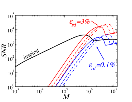
We first compute SNRs for both inspiral and ringdown for events at $D_{L}=3~{}$Gpc, corresponding to a redshift $z\simeq 0.54$, based on our choice for cosmological parameters cosmology . To compute the inspiral SNR we adopt the method discussed in Ref. BBW . We perform an angle-average over pattern functions, assuming that we observe the last year of inspiral and that we can extrapolate the LISA noise curve down to a frequency $f\simeq 10^{-5}~{}$Hz. Following the common practice, we truncate the signal-to-noise ratio integral, Eq. (13), using an upper cutoff frequency determined by the conventional Schwarzschild ISCO for a black hole of mass $M$.

We compute the ringdown SNR for the fundamental mode with $l=m=2$; calculations for different values of $l$ and $m$ yield similar results, the SNR depending mainly on the ringdown efficiency in a given mode. We use the FH SNR (21) and adopt the $\delta$-function approximation (21b). Performing the “full” integral over the Breit-Wigner distribution (21a) we obtain essentially indistinguishable results, except for a small ($\lesssim~{}10\%$) disagreement in the mass/frequency region dominated by the white-dwarf confusion noise (this statement is made more quantitative in Fig. 19 of Appendix A).

Figure 7: Comparison of the SNR for inspiral and ringdown waveforms. In the left panel we use the Barack-Cutler noise-curve; in the right panel we use the same noise curve, but we do not include white-dwarf confusion noise. The thick (black) line marked by “inspiral” is the (angle-averaged) SNR for the inspiral of two equal-mass black holes at $D_{L}=3~{}$Gpc. The other sets of lines (red and blue in color versions) show the SNR for the $l=m=2$ mode using the $\delta$-function approximation, assuming a ringdown efficiency $\epsilon_{\rm rd}=3\%$ and $0.1\%$ respectively. Solid, dashed and dot-dashed lines correspond to $j=0$ (Schwarzschild), $j=0.8$ and $j=0.98$ respectively.

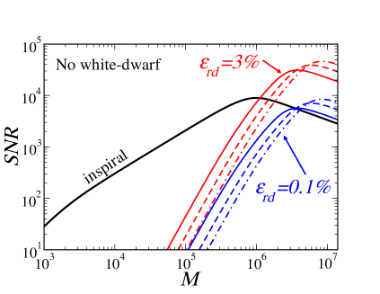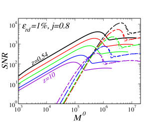
The results are shown in Fig. 7. These plots can be viewed as an updated version of Fig. 6 in FH. Compared to FH we use a better model of the LISA noise curve (cf. Appendix C). In particular, a comparison of the left and right panels illustrates the effect of white-dwarf confusion noise on the expected SNR. In both panels of Fig. 7, the thick curve marked by “inspiral” represents the inspiral SNR for two equal-mass black holes with total mass $M$ equal to the mass of the final black hole.

The ringdown SNR in Fig. 7 is shown as sets of solid, dashed and dot-dashed lines, corresponding to the limiting case of a Schwarzschild black hole with $j=0$, an intermediate rotation rate $j=0.8$, and a near extremal rate $j=0.98$, respectively. The intermediate value seems astrophysically quite plausible, based on the best available astrophysical observations and on theoretical models of merger and accretion (see, e.g. gammie ). FH considered only ($j=0.98$). For the ringdown efficiency we show the optimistic value $\epsilon_{\rm rd}=3~{}\%$ considered by FH, as well as a pessimistic value $\epsilon_{\rm rd}=0.1~{}\%$. The latter value corresponds to the present best estimates for the energy emitted in a maximally symmetric merger, i.e. in the head-on collision of equal-mass black holes (see sperhake and references therein). For unequal-mass mergers, FH suggest (interpolating between numerical and perturbative results) an energy scaling of the form $(4\mu/M)^{2}$, where $\mu$ is the reduced mass.

The general features of the SNR curves are easy to understand. The SNR is basically proportional to the inverse of the noise power spectral density $S_{h}(f)$. It has a maximum in the mass range $M\sim 10^{6}M_{\odot}$ corresponding to the frequency $f\sim 10^{-2}~{}$Hz at which LISA is most sensitive. If we include white-dwarf confusion noise (left panel) we observe the appearance of a dip in the SNR at masses $M$ of the order of a few times $10^{6}M_{\odot}$. The black hole at our Galactic Center has an estimated mass $M\simeq 3.7\pm 0.2\times 10^{6}~{}M_{\odot}$ (see eg. narayan ), so an accurate modelling of the white-dwarf confusion noise might be very important for detection of black hole ringdown from galactic centers. In this paper, unless otherwise stated, we will include white-dwarf confusion noise in all of our numerical calculations.

Fig. 7 illustrates that, even under pessimistic assumptions, the ringdown SNR is generally comparable to the inspiral SNR. Reducing the rotation rate does not have a dramatic effect, degrading the SNR of corotating modes by factors of order unity. The crucial element for detectability is the fraction of mass-energy $\epsilon_{\rm rd}$ going into each mode. Note that Eq. (25) implies that $\rho\sim\sqrt{\epsilon_{\rm rd}}$.

FH and Ref. rhook pointed out that, depending on the ringdown efficiency, there might be a “critical mass” at which black hole ringdown becomes dominant over inspiral. Assuming an efficiency $\epsilon_{\rm rd}=1\%$ and a final black hole angular momentum $j=0.997$, Ref. rhook found that the SNR is greater in the ringdown signal for $M\gtrsim 10^{6}M_{\odot}$ when $z=1$. Their result is consistent with our Fig. 7; in addition, we find that this “critical mass” for the transition from inspiral to ringdown dominance depends only weakly on $j$, being more sensitive to the efficiency $\epsilon_{\rm rd}$.

Ringdown efficiency plays a very important role in the ringdown SNR. Unfortunately, numerical relativity simulations do not provide us with reliable estimates of $\epsilon_{\rm rd}$ BCW2 . Ref. BCD provides alternative, semianalytical estimates of the energy radiated in the plunge and ringdown phases for Earth-based detectors; unfortunately, an extrapolation of those results to binaries of relevance for LISA is not available. Given our ignorance of $\epsilon_{\rm rd}$, it makes sense to ask the following question: how much energy must be channelled into a given mode in order for it to be detectable?

The answer to this question is provided by Fig. 1 in Sec I, where we assume $\rho=10$ as a criterion for detectability and we show the fundamental mode of a Kerr black hole with $l=m=2$. The result is encouraging: even in the pessimistic situation of a head-on collision $\epsilon_{\rm rd}=10^{-3}$, we can reasonably expect LISA to detect all mergers yielding a black hole of mass $M\gtrsim 10^{5}M_{\odot}$. Even accounting for the fact that $\epsilon_{\rm rd}$ may be lower for unequal mass mergers, the prospects for detection are still encouraging.

Figure 8: Dependence of the SNR on redshift, for both inspiral (continuous lines) and ringdown (dashed and dot-dashed lines). We choose a ringdown efficiency $\epsilon_{\rm rd}=1\%$ and consider the cases $j=0$, $j=0.8$ and $j=0.98$. From top to bottom the lines in each panel correspond to $z=0.54$ (black in color versions; $D_{L}=3$ Gpc), $z=1$ (red), $z=2$ (green), $z=5$ (blue) and $z=10$ (purple). The dashed lines are obtained from the full integral, the dot-dashed lines use the $\delta$-function approximation.

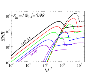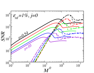
The cosmological redshift affects the detectability window and the SNR both for inspiral and for ringdown waves, both through the decreasing signal strength with distance and through shifting the relevant frequencies to different parts of the LISA noise spectrum. Fig. 8 shows the results of numerical calculations of the SNR. For the ringdown signal, we pick a ”best guess” for the efficiency $\epsilon_{\rm rd}$ of $1\%$, intermediate between the $3\%$ of FH and the $0.1\%$ from head-on collisions. Each plot gives the SNR as a function of $M^{0}$ (mass in the source frame) for a different value of $j$ (left to right, $j=0$, $j=0.8$ and $j=0.98$). From top to bottom, the curves show sources at redshifts $z=0.54,\,1,\,2,\,5$ and $10$. The continuous lines are the inspiral SNR, the dashed lines are obtained from the full integral, the dot-dashed lines use the $\delta$-function approximation. The inspiral SNR is (somewhat arbitrarily) truncated at the (large) value of the mass for which the starting frequency (which we pick to be one year before the ISCO, as in BBW ) becomes lower than $10^{-5}$ Hz.

IV Parameter estimation by detection of a single mode

IV.1 Analytic results

In this Section we will go beyond the issue of detectability and try to answer a different question: given the detection of a single QNM, what can we learn about the black hole parameters? To estimate the black hole parameters from ringdown waveforms, we use the standard technique of parameter estimation in matched filtering. By maximizing the correlation between a template gravitational waveform that depends on a set of parameters $\theta^{a}$ (for example, the black hole mass and angular momentum) and a measured signal, matched filtering provides a natural way to estimate the parameters of the signal and their errors. With a given noise spectral density for the detector, $S_{h}(f)$, one defines the inner product between two signals $h_{1}(t)$ and $h_{2}(t)$ by

$$(h_{1}|h_{2})\equiv 2\int_{0}^{\infty}\frac{{\tilde{h}_{1}}^{*}\tilde{h}_{2}+{\tilde{h}_{2}}^{*}\tilde{h}_{1}}{S_{h}(f)}df\,,$$ (33)

where $\tilde{h}_{1}(f)$ and $\tilde{h}_{2}(f)$ are the Fourier transforms of the respective gravitational waveforms $h(t)$. The components of the “Fisher matrix” $\Gamma_{ab}$ are then given by

$$\Gamma_{ab}\equiv\left(\frac{\partial h}{\partial\theta^{a}}\mid\frac{\partial h}{\partial\theta^{b}}\right)\,,$$ (34)

In the limit of large SNR, if the noise is stationary and Gaussian, the probability that the gravitational-wave signal $s(t)$ is characterized by a given set of values of the source parameters $\theta^{a}$ is

$$p(\mbox{\boldmath$\theta$}|s)=p^{(0)}(\mbox{\boldmath$\theta$})\exp\left[-\frac{1}{2}\Gamma_{ab}\delta\theta^{a}\delta\theta^{b}\right]\,.$$ (35)

where $\delta\theta^{a}=\theta^{a}-{\hat{\theta}}^{a}$, and $p^{(0)}(\mbox{\boldmath$\theta$})$ represents the distribution of prior information. An estimate of the rms error, $\Delta\theta^{a}=(\langle(\delta\theta^{a})^{2}\rangle)^{1/2}$, in measuring the parameter $\theta^{a}$ can then be calculated, in the limit of large SNR, by taking the square root of the diagonal elements of the inverse of the Fisher matrix,

$$\Delta\theta^{a}=\sqrt{\Sigma^{aa}}\,,\qquad\Sigma=\Gamma^{-1}\,.$$ (36)

The correlation coefficients between two parameters $\theta^{a}$ and $\theta^{b}$ are given by

$$c_{ab}=\Sigma^{ab}/\sqrt{\Sigma^{aa}\Sigma^{bb}}\,.$$ (37)

We consider a waveform given by Eq. (10), with the $S_{lmn}$ assumed to be real,

$$h_{+} = \frac{M}{r}{\cal A}_{lmn}^{+}e^{-\pi f_{lmn}t/Q_{lmn}}\cos\left[2\pi f_{lmn}t+\phi_{lmn}^{+}\right]S_{lmn}(\iota,\beta)\,,$$ (38a)

$$h_{\times} = \frac{M}{r}{\cal A}_{lmn}^{\times}e^{-\pi f_{lmn}t/Q_{lmn}}\sin\left[2\pi f_{lmn}t+\phi_{lmn}^{\times}\right]S_{lmn}(\iota,\beta)\,.$$ (38b)

We also define

$$\frac{M}{r}{\cal A}_{lmn_{1}}^{+}\equiv A^{+}\,,\qquad\frac{M}{r}{\cal A}_{lmn_{1}}^{\times}\equiv A^{\times}\equiv A^{+}{\rm N_{\times}}\,,$$ (39)

where $N_{\times}$ is some numerical factor, and

$$\phi_{lmn}^{\times}=\phi_{lmn}^{+}+\phi_{lmn}^{0}\,.$$ (40)

Assuming that we know $N_{\times}$ and $\phi_{lmn}^{0}$, this waveform is dependent on four parameters ($A^{+}$, $\phi_{lmn}^{+}$, $M$, $j$); otherwise it depends on six parameters ($A^{+}$, $A^{\times}$, $\phi_{lmn}^{+}$, $\phi_{lmn}^{\times}$, $M$, $j$). A popular choice for $N_{\times}$ fhh ; rhook is to assume that the distribution of the strain in the two polarizations mimics that of the inspiral phase: $N_{\times}=-2(\hat{\mathbf{L}}\cdot\hat{\mathbf{n}})/[1+(\hat{\mathbf{L}}\cdot\hat{\mathbf{n}})^{2}]$, where $\hat{\mathbf{L}}$ is the orientation of the binary’s angular momentum and $\hat{\mathbf{n}}$ is a unit vector describing the binary’s position in the sky. Fortunately, we will see that the errors have a very weak dependence on the number of parameters and on the (uncertain) value of the parameters $N_{\times}$ and $\phi_{lmn}^{0}$.

Assuming constant noise over the bandwidth of the signal, or taking the $\delta$-function approximation, and using the FH doubling convention, we get the SNR (20). In this approximation, errors and correlation coefficients can be computed analytically using Mathematica or Maple. The full expressions are lengthy and unenlightening, and we have implemented them numerically in a Fortran code.

We first calculate the Fisher matrix in the parameter basis of $(A^{+},\,\phi_{lmn}^{+},\,f_{lmn},\,Q_{lmn})$, where it takes on a simpler form:

$$\Gamma_{A^{+}A^{+}} = \frac{\gamma}{(A^{+})^{2}}\left(1+4Q_{lmn}^{2}-\beta\right)\,,$$ (41a)

$$\Gamma_{A^{+}\phi_{lmn}^{+}} = \frac{\gamma}{A^{+}}\alpha\,,$$ (41b)

$$\Gamma_{A^{+}f_{lmn}} = -\frac{\gamma}{2A^{+}f_{lmn}}\left(1+4Q_{lmn}^{2}-\beta\right)\,,$$ (41c)

$$\Gamma_{A^{+}Q_{lmn}} = \frac{\gamma}{2A^{+}Q_{lmn}}\frac{1}{1+4Q_{lmn}^{2}}\left[(1+4Q_{lmn}^{2})^{2}-(1-4Q_{lmn}^{2})\beta\right]\,,$$ (41d)

$$\Gamma_{\phi_{lmn}^{+}\phi_{lmn}^{+}} = \gamma\left(1+4Q_{lmn}^{2}+\beta\right)\,,$$ (41e)

$$\Gamma_{\phi_{lmn}^{+}f_{lmn}} = -\frac{\gamma}{2f_{lmn}}\alpha\,,$$ (41f)

$$\Gamma_{\phi_{lmn}^{+}Q_{lmn}} = \frac{\gamma}{2Q_{lmn}}\left(\frac{1-4Q_{lmn}^{2}}{1+4Q_{lmn}^{2}}\right)\alpha\,,$$ (41g)

$$\Gamma_{f_{lmn}f_{lmn}} = \frac{\gamma}{2f_{lmn}^{2}}\left[(1+4Q_{lmn}^{2})^{2}-\beta\right]\,,$$ (41h)

$$\Gamma_{f_{lmn}Q_{lmn}} = -\frac{\gamma}{2f_{lmn}Q_{lmn}}\frac{1}{1+4Q_{lmn}^{2}}\left[(1+4Q_{lmn}^{2})^{2}-(1-4Q_{lmn}^{2})\beta\right]\,,$$ (41i)

$$\Gamma_{Q_{lmn}Q_{lmn}} = \frac{\gamma}{2Q_{lmn}^{2}}\frac{1}{(1+4Q_{lmn}^{2})^{2}}\left[(1+4Q_{lmn}^{2})^{3}-(1-12Q_{lmn}^{2})\beta\right]\,,$$ (41j)

where

$$\alpha = \sin^{2}\psi\sin 2\phi_{lmn}^{\times}-\cos^{2}\psi\sin 2\phi_{lmn}^{+}\,,$$ (42a)

$$\beta = \sin^{2}\psi\cos 2\phi_{lmn}^{\times}-\cos^{2}\psi\cos 2\phi_{lmn}^{+}\,,$$ (42b)

$$\gamma = \frac{A^{2}Q_{lmn}}{40\pi^{2}f_{lmn}(1+4Q_{lmn}^{2})}\,,$$ (42c)

with $\cos\psi\equiv 1/\sqrt{1+N_{\times}^{2}}$, $\sin\psi\equiv N_{\times}/\sqrt{1+N_{\times}^{2}}$ and $A^{2}=(A^{+})^{2}(1+N_{\times}^{2})=(A^{+})^{2}+(A^{\times})^{2}$. Note that, in this notation, $\rho_{FH}^{2}=\gamma(1+4Q_{lmn}^{2}-\beta)$.

We note that the Fisher matrix written in terms of the frequency and damping time is usually simpler finn ; kaa than that in terms of mass and angular momentum; however we prefer to deal directly with measurements of $j$ and $M$. In Sec. VII, to estimate QNM resolvability, we will work in terms of frequencies and quality factors.

The transformation from the $(A^{+},\,\phi_{lmn}^{+},\,f_{lmn},\,Q_{lmn})$ basis to the $(A^{+},\,\phi_{lmn}^{+},\,M,\,j)$ basis is straightforward, namely, for any index $k$,

$$\Gamma_{k\,M} = -(f_{lmn}/M)\Gamma_{k\,f_{lmn}}\,,$$

$$\Gamma_{k\,j} = f_{lmn}^{\prime}\Gamma_{k\,f_{lmn}}+Q_{lmn}^{\prime}\Gamma_{k\,Q_{lmn}}\,,$$ (43)

where $f_{lmn}^{\prime}\equiv df_{lmn}/dj$ and $Q_{lmn}^{\prime}\equiv dQ_{lmn}/dj$.

Converting to this basis and inverting the Fisher matrix, we find, to leading order in $Q_{lmn}^{-1}$, the errors

$$\sigma_{j} = \frac{1}{\rho_{\rm FH}}\left|2\frac{Q_{lmn}}{Q_{lmn}^{\prime}}\left(1+\frac{1+4\beta}{16Q_{lmn}^{2}}\right)\right|\,,$$ (44a)

$$\sigma_{M} = \frac{1}{\rho_{\rm FH}}\left|2\frac{MQ_{lmn}f_{lmn}^{\prime}}{f_{lmn}Q_{lmn}^{\prime}}\left(1+\frac{1+4\beta}{16Q_{lmn}^{2}}\right)\right|\,,$$ (44b)

$$\sigma_{A^{+}} = \frac{\sqrt{2}A^{+}}{\rho_{\rm FH}}\left|1+\frac{3\beta}{8Q_{lmn}^{2}}\right|\,,$$ (44c)

$$\sigma_{\phi_{lmn}^{+}} = \frac{1}{\rho_{\rm FH}}\left|1-\frac{\beta}{4Q_{lmn}^{2}}\right|\,,$$ (44d)

and the correlation coefficients

$$r_{jM} = {\rm sgn}(f_{lmn}^{\prime})\times\left(1-\frac{f_{lmn}^{2}Q_{lmn}^{\prime 2}}{16Q_{lmn}^{4}f_{lmn}^{\prime 2}}\right)+{\cal O}(1/Q^{6})\,,$$ (45a)

$$r_{jA^{+}} = -\frac{1}{\sqrt{2}}\left(1-\frac{1-6\beta}{16Q_{lmn}^{2}}\right)+{\cal O}(1/Q^{4})\,,$$ (45b)

$$r_{MA^{+}} = -\frac{1}{\sqrt{2}}\left(1-\frac{1-6\beta}{16Q_{lmn}^{2}}\right)+{\cal O}(1/Q^{3})\,,$$ (45c)

$$r_{j\phi_{lmn}^{+}} = \frac{\alpha}{2Q_{lmn}^{2}}-\frac{7-8\beta}{32Q_{lmn}^{4}}+{\cal O}(1/Q^{6})\,,$$ (45d)

$$r_{M\phi_{lmn}^{+}} = \frac{\alpha}{2Q_{lmn}^{2}}-\frac{7-8\beta}{32Q_{lmn}^{4}}+{\cal O}(1/Q^{6})\,,$$ (45e)

$$r_{A^{+}\phi_{lmn}^{+}} = -\frac{3\alpha}{4\sqrt{2}Q_{lmn}^{2}}+\frac{\alpha(10-11\beta)}{32\sqrt{2}Q_{lmn}^{4}}+{\cal O}(1/Q^{6})\,.$$ (45f)

In calculating derivatives of the waveforms (38) with respect to $M$ and $j$ (or with respect to $f_{lmn}$ and $Q_{lmn}$), we have ignored derivatives of the spheroidal harmonics themselves. The $S_{lmn}$ are functions of $a\omega_{lmn}=j{\cal F}_{lmn}$ which is a function of $j$ only. However, the $S_{lmn}$ may be expanded in powers of $j{\cal F}_{lmn}$, in the form

$$S_{lmn}=Y_{lm}+(j{\cal F}_{lmn})\,\sum_{l^{\prime}\neq l}c_{l^{\prime}lm}Y_{l^{\prime}m}+O(j{\cal F}_{lmn})^{2}\,,$$ (46)

where $Y_{lm}$ denotes a spin-weighted spherical harmonic, and $c_{l^{\prime}lm}$ are related to Clebsch-Gordan coefficients. As a result, derivatives of the $S_{lmn}$ with respect to $j$ will be linear in derivatives of $j{\cal F}_{lmn}$, and because of the orthogonality of the spin-weighted spherical harmonics, inner products of $S_{lmn}$ with $S_{lmn}^{\prime}$ and of $S_{lmn}^{\prime}$ with itself will be at least quadratic in $j{\cal F}_{lmn}$ and its derivatives. At least for small $j{\cal F}_{lmn}$, we may expect these contributions to be small relative to the main contribution obtained by ignoring these derivatives. Nevertheless, the effect of this approximation should be explored further.

The diagonal elements of the correlation matrix $r_{ii}=1$ for all $i$. The ${\rm sgn}(f_{lmn}^{\prime})$ in $r_{jM}$ comes from a $\sqrt{f_{lmn}^{\prime 2}}/f_{lmn}^{\prime}=|f_{lmn}^{\prime}|/f_{lmn}^{\prime}$. It implies that $j$ and $M$ have a positive correlation for corotating and axisymmetric modes ($m\geq 0$), but they are anticorrelated for counterrotating modes ($m<0$): this is basically determined by the different sign of $f_{lmn}^{\prime}$ for the two classes of modes (see eg. Fig. 5).

The calculation using the EF convention proceeds along similar lines; the results are very similar, and they are reported in Appendix B. The calculation for a six-dimensional Fisher matrix is straightforward, and is also relegated to Appendix B.

The large-$Q_{lmn}$ expansions are typically accurate as long as $Q_{lmn}^{\prime}/Q_{lmn}$ is not very large (see Fig. 10 below, where this statement is made more quantitative). An analytic parametrization for $\sigma$ can be obtained by combining the SNR formula (30) and (31) with the QNM fits, whose coefficients are provided in Tables 8, 9 and 10.

An important check is that the errors on $M$ and $j$ (and the correlation between these parameters), as predicted by Finn finn , agree with ours. This is not a trivial check, since Finn uses a different parametrization of the waveform. In particular, it is easy to check that Finn’s expressions for the errors, his Eqs. (4.20a) and (4.20b), agree with ours to leading order in $Q_{lmn}^{-1}$; so does Finn’s expression for the correlation coefficient, his Eq. (4.20e). The fact that only high-order corrections in $Q_{lmn}^{-1}$ depend on the parametrization is a reassuring feature of the Fisher matrix calculation (see Appendix B).

Some general comments on Eqs. (44) and (45) are in order. First, by combining Eqs. (44a) and (44b) with Eq. (30), we see that the accuracy in measuring $M$ and $j$ can be very high under the right circumstances, namely,

$$\frac{\sigma_{M}}{M} \simeq 6.8\times 10^{-3}\times h_{lmn}(j){\cal F}_{lmn}\times\left(\frac{10^{-4}}{\epsilon_{\rm rd}}\right)^{1/2}\left(\frac{S_{h}(f_{lmn})}{S_{0}}\right)^{1/2}\left(\frac{D_{L}(z)}{1~{}{\rm Gpc}}\right)\left(\frac{10^{6}M_{\odot}}{(1+z)M}\right)^{3/2}\,,$$ (47a)

$$\sigma_{j} \simeq 6.8\times 10^{-3}\times g_{lmn}(j){\cal F}_{lmn}\times\left(\frac{10^{-4}}{\epsilon_{\rm rd}}\right)^{1/2}\left(\frac{S_{h}(f_{lmn})}{S_{0}}\right)^{1/2}\left(\frac{D_{L}(z)}{1~{}{\rm Gpc}}\right)\left(\frac{10^{6}M_{\odot}}{(1+z)M}\right)^{3/2}\,.$$ (47b)

Notice that the measurement error is small (less than a percent), even under the very pessimistic assumption that a SMBH with $M\sim 10^{6}~{}M_{\odot}$ radiates only a modest fraction $E_{\rm GW}\sim 10^{-4}M$ of its mass. The functions $g_{lmn}(j)=Q_{lmn}/Q_{lmn}^{\prime}$ and $h_{lmn}(j)=(Q_{lmn}f_{lmn}^{\prime})/(Q_{lmn}^{\prime}f_{lmn})$ depend on the particular mode we consider and on the black hole’s angular momentum; they are typically of order unity. For example, using the fitting relations in Appendix E, we find that, for the fundamental mode with $l=m=2$ of a Schwarzschild black hole, these factors take the values $g_{lmn}(0)=2.992$, $h_{lmn}(0)=1.214$. So, for a non-rotating black hole the error in angular momentum is slightly larger than the error on the mass. For a near-extremal black hole we have $g_{lmn}(0.98)=0.043$, $h_{lmn}(0.98)=0.234$, and the error in angular momentum is now smaller than the error in the mass. We will see that this reversal of the magnitude of the errors for near-extremal black holes is typical of corotating modes, but does not hold true for counterrotating modes.

Figure 9: $Q_{lmn}/Q_{lmn}^{\prime}$ for the fundamental mode with $l=2$ (left) and $l=4$. Solid lines refer to $m>0$, dotted lines to $m=0$, dashed lines to $m<0$, and different shades (colors) denote different values of $m$, as indicated. Notice that this factor increases with $j$ when $m>0$ and decreases with $j$ when $m=-2$. The factor blows up as $j\to 0$ for $m=0$, and as $j\to j_{\rm crit}$ for certain values of $m<0$. This explains most qualitative features of the error plots.

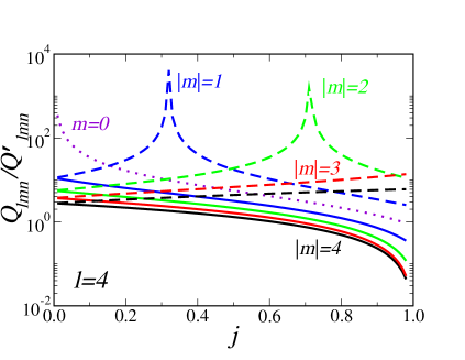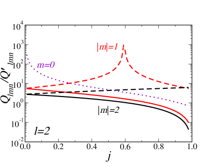
To leading order in a large-$Q_{lmn}$ expansion the errors on angular momentum and mass, Eqs. (44a) and (44b), are proportional to $Q_{lmn}/Q_{lmn}^{\prime}$. In Fig. 9 we plot this quantity as a function of $j$ for different modes. From the plot we can anticipate a few salient features. First of all, errors should decrease with rotation for corotating modes ($m>0$). This was already pointed out in Refs. echeverria ; finn . However, errors should increase with rotation for counterrotating modes ($m<0$); even worse, at those “critical values” of $j$ for which $Q_{lmn}^{\prime}=0$ the errors for counterrotating modes blow up. Fig. 9 shows that, typically, this phenomenon is present for counterrotating modes with $|m|\leq l/2$. Finally, we can anticipate that $Q_{lmn}/Q_{lmn}^{\prime}$ (hence the error) will blow up as $j\to 0$ for modes with $m=0$.

Figure 10: Comparison between different approaches to compute the error (multiplied by the SNR) for the fundamental mode for $(l,m)=(2,2)$ and $(2,-1)$. Solid lines use the numerical implementation of the full expressions obtained by Mathematica, and a numerical calculation of the derivatives of $Q_{lmn}$ and $f_{lmn}$. Dashed and dotted lines use expressions for the Fisher matrix to leading order in $1/Q_{lmn}$; derivatives of $Q_{lmn}$ and $f_{lmn}$ are evaluated numerically for the former, and using the fitting functions given in Appendix E for the latter. Black (red) lines refer to calculations of the error in $j$ ($M$) using the FH “doubling prescription”. The plot shows that all these different calculations are in excellent agreement with each other. However, sometimes using the fits can produce only order-of-magnitude estimates of the errors: this happens for counterrotating modes, where an accurate calculation of the derivatives of $Q_{lmn}$ and $f_{lmn}$ is more important (dotted lines in the right panel deviate significantly from the “true” answer obtained by taking numerical derivatives of the QNM tables). Finally (and only in the right panel) we plot, in blue, results obtained using Eqs. (4.20a), (4.20b) in Finn’s paper finn , a numerical implementation of the full expressions obtained by Mathematica, and a numerical calculation of the derivatives of $Q_{lmn}$ and $f_{lmn}$. Finn’s formula would lie on top of the other lines in the left plot (for $l=m=2$), but it gives a slightly different prediction for the errors on the counterrotating mode with $l=2$, $m=-1$.

IV.2 Numerical results

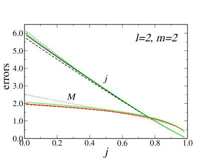
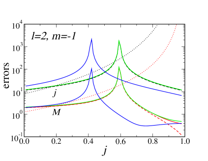
Our expectations are validated by an explicit numerical calculation of the errors. We carry out this calculation in different ways, and in Fig. 10 we show that results obtained from these different methods are usually in very good agreement. The most reliable calculation is “fully numerical” (solid lines in Fig. 10), in the sense that it involves no semianalytical approximations. In this calculation we use the “complete” expressions for the errors obtained using Mathematica. For increased accuracy, for any given value of $j$ we interpolate our numerical tables of the QNMs by fifth-order polynomials and evaluate “numerically” the derivatives $f_{lmn}^{\prime}$ and $Q_{lmn}^{\prime}$ by taking derivatives of these interpolating polynomials at the given $j$. Dashed lines investigate the accuracy of leading order Taylor expansions for large $Q_{lmn}$ of the errors, such as Eqs. (44), and use these “local” interpolating polynomials to compute $f_{lmn}^{\prime}$ and $Q_{lmn}^{\prime}$. Finally, dotted lines use Taylor expansions of the errors and evaluate the derivatives $f_{lmn}^{\prime}$ and $Q_{lmn}^{\prime}$ using the (somehow less accurate) “global” fits of the QNM tables we provide in Appendix E.

Overall, different choices for the doubling convention and/or for the number of parameters yield consistent results for the errors. In isolated, unfortunate cases the “global” fits of Appendix E, being valid in the whole range $j\in[0,1]$ but not very accurate for certain values of $j$, provide only an order-of-magnitude estimate of the errors. This happens, for example, when we consider counterrotating modes with $l=2$ and $|m|<l/2$ (see eg. the right panel of Fig. 10). It also happens for modes with $m=0$, in the limit $j\to 0$. The reason is that in these cases $Q_{lmn}$ has a minimum, and $Q_{lmn}/Q_{lmn}^{\prime}$ blows up. This behavior is only captured by an accurate local fit of the QNM data (such as the polynomial fit we use to compute derivatives). The bottom line is that the global fits of Appendix E are generally inaccurate to compute measurement errors whenever the numerical QNM tables are such that $Q_{lmn}^{\prime}\simeq 0$ for some value of $j$.

Figure 11: Correlation between the mass and angular momentum parameters for the fundamental mode and different values of $(l,m)$. For counterrotating modes $j$ and $M$ are actually anticorrelated ($r_{jM}<0$), and we plot the modulus of the correlation. The solid line uses the numerical implementation of the full expressions obtained by Mathematica, and a numerical calculation of the derivatives of $Q_{lmn}$ and $f_{lmn}$. The dashed line uses an expansion to leading order in $1/Q_{lmn}$ of the correlation matrix, and a numerical calculation of the derivatives of $Q_{lmn}$ and $f_{lmn}$. The dotted line uses again a Taylor expansion, but this time we evaluate the derivatives of $Q_{lmn}$ and $f_{lmn}$ using the fitting functions given in Appendix E. The minimum in the correlation between mass and angular momentum (for $l=m=2$) disappears when we use the numerical derivatives. The behavior of $r_{jM}$, as computed numerically, is qualitatively consistent with the entry marked by $f_{Ma}$ in Echeverria’s Table II echeverria , so the fake minimum really seems to be due to the inaccuracy of the fit.

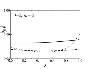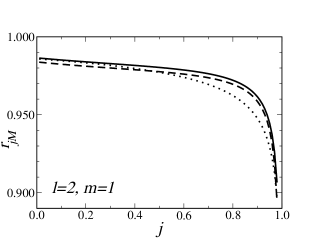
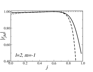
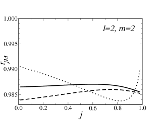
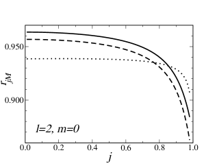
Let us now turn to correlation coefficients. To leading order, the correlation coefficient between mass and angular momentum $r_{jM}=1$ for all modes. This high correlation between mass and angular momentum was first pointed out by Echeverria echeverria for the fundamental mode with $l=m=2$. Echeverria suggested that, if we have some independent and more precise measurement of either the mass or the angular momentum (but not both) we could exploit this strong correlation to obtain an almost equally better estimate of the other parameter. This means that mass measurements of SMBHs (as inferred from the Keplerian orbits of the surrounding stars, for example) could be used in conjuction with gravitational-wave observations to provide accurate determinations of the hole’s angular momentum. Mass and angular momentum are also strongly correlated with the wave’s amplitude: to leading order, $|r_{jA}|=|r_{MA}|=1/\sqrt{2}\simeq 0.707$. On the contrary, the polarization phase $\phi_{lmn}$ is very weakly correlated with the other parameters: the leading-order term is proportional to $Q_{lmn}^{-2}$ when we use the FH convention, and to $Q_{lmn}^{-1}$ when we use the EF convention, Eq. (63). Independently of our convention and of the parametrization of the waveform, this small correlation implies that we can expect the phase to be irrelevant in measuring the black hole mass and angular momentum.

In Fig. 11 we present results from a numerical calculation of the correlation coefficient $r_{jM}$ (which is, again, independent of different choices on the doubling convention and/or on the number of parameters).

Figure 12: Errors in measurements of different parameters for the fundamental mode with different values of $(l,m)$, as functions of the angular momentum parameter $j$. Solid (black) lines give $\rho\sigma_{j}$, dashed (red) lines $\rho\sigma_{M}/M$, dot-dashed (green) lines $\rho\sigma_{A}/A$, dot-dot-dashed (blue) lines $\rho\sigma_{\phi_{lmn}}$.

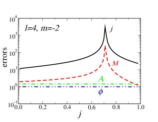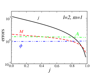
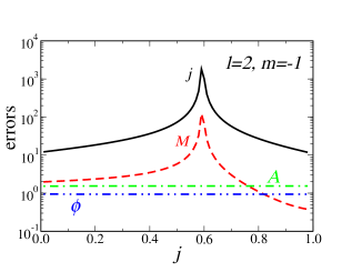
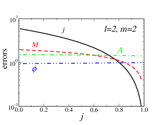
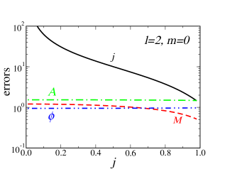
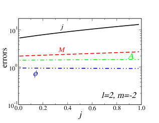
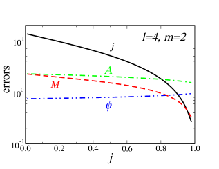
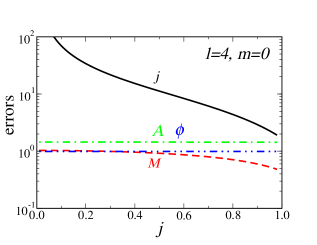
Fig. 12 shows the errors in different parameters rescaled by the SNR for different QNMs. All errors scale with the inverse of the SNR, $\sigma_{x}\sim\rho^{-1}$, and all information about the detector is contained in the SNR. Therefore we plot the quantities $(\rho\sigma_{j},~{}\rho\sigma_{M}/M,~{}\rho\sigma_{A}/A,~{}\rho\sigma_{\phi_{lmn}})$, which are, in some sense,“universal”: they do not depend on the specifics of the LISA noise curve, but only on intrinsic features of the gravitational waveform emitted by the perturbed black hole.

In the plot, we use the FH convention and consider a four-dimensional correlation matrix, but results would not have changed much had we used the EF convention and/or a six dimensional correlation matrix. We use the numerical implementation of the full expressions obtained by Mathematica, and a numerical calculation of the derivatives of $Q_{lmn}$ and $f_{lmn}$. Once again, results do not change appreciably if we use a Taylor expansion to leading order in $1/Q_{lmn}$ of the correlation matrix, and a numerical calculation of the derivatives of $Q_{lmn}$ and $f_{lmn}$. Even if we use the QNM fits of Appendix E we get very similar results: only for counterrotating modes do those fits fail to reproduce the location of the peak we can see for $(l=2,~{}m=-1)$ and $(l=4,~{}m=-2)$.

The general features emerging from Fig. 12 agree with the expectations drawn from Fig. 9. Errors on mass and angular momentum decrease with rotation for corotating modes ($m>0$), but they increase with rotation for counterrotating modes ($m<0$), blowing up at those “critical values” of $j$ for which $Q_{lmn}^{\prime}=0$ (which occurs for counterrotating modes with $|m|\leq l/2$). The error on $j$ goes to infinity as $j\to 0$ when we consider modes with $m=0$, but the error on $M$ stays finite in this same limit. Errors on the amplitude $A$ and phase $\phi_{lmn}$ usually have a very weak dependence on $j$.

Figure 13: Errors in angular momentum $\sigma_{j}$ (black) and mass $\sigma_{M}/M$ (red) for: $l=m=2$ (top left), $l=2$, $m=0$ (top center), $l=2$, $m=-2$ (top right); $l=4$, $m=2$ (bottom left), $l=4$, $m=0$ (bottom center), $l=4$, $m=-2$ (bottom right), for a source at $D_{L}=3\,{\rm Gpc}$ with $\epsilon_{\rm rd}=3\%$. Solid lines refer to $j=0$, dashed lines to $j=0.8$, dot-dashed lines to $j=0.98$. Errors scale with $\rho^{-1}$, hence they are proportional to $\epsilon_{\rm rd}^{-1/2}$.

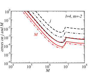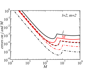
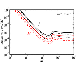
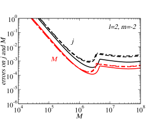
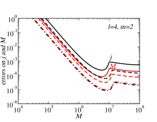
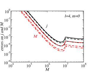
Of course Fig. 12 tells only part of the story, because it does not involve any information about the actual specifics of the LISA noise. Fig. 13 shows the actual errors computed using the Barack-Cutler noise curve including white-dwarf confusion noise described in Appendix C. We use the $\delta$-function approximation to compute $\rho$, and consider different angular indices $(l,m)$. For concreteness we assume that our source is located at $D_{L}=3$ Gpc and has a ringdown efficiency $\epsilon_{\rm rd}=3\%$ for each mode. However, even in the worst-case equal-mass merger scenario ($\epsilon_{\rm rd}=0.1\%$) errors would only increase by a modest factor $\sqrt{30}\simeq 5.5$.

The angular momentum dependence can most easily be understood looking at the “universal” Fig. 12. As an example, focus on the mode with $l=m=2$. From Fig. 12 we see that the error on $j$ is larger than the error on $M$ for $j\lesssim 0.8$, comparable to it for $j\simeq 0.8$, and smaller than the error on $M$ for $j\gtrsim 0.8$: this is precisely what we see in the top-left panel of Fig. 13. Including information on the noise, Fig. 13 gives a good quantitative idea of the kind of accuracy we can achieve if we try to measure mass and angular momentum of black holes with LISA. Numerical results are in good agreement with our expectations based on Eqs. (47a) and (47b). Errors become unacceptably large only for black hole masses $M\lesssim 10^{5}M_{\odot}$, but in general we can expect excellent accuracies: the measurement of a single ringing event can provide the mass and angular momentum of black holes with $M\gtrsim 5\times 10^{5}M_{\odot}$ with errors smaller than one part in $10^{2}$, and (in the most optimistic cases, eg. for black holes of mass $\sim 5\times 10^{6}M_{\odot}$) smaller than one part in $10^{5}$.

To generalize our results to other values of $\epsilon_{\rm rd}$ it is enough to recall that the SNR scales with the square root of $\epsilon_{\rm rd}$, $\rho\sim\epsilon_{\rm rd}^{1/2}$, so the errors scale like $\epsilon_{\rm rd}^{-1/2}$. Numerical simulations suggest that for the first overtone $\epsilon_{\rm rd}$ should be smaller by a factor $10^{2}-10^{4}$ when compared to the fundamental mode. This means that the error will be $\sim 10-10^{2}$ times larger than the value plotted in Fig. 13. Accurate tests of the no-hair theorem involve the measurement of two QNM frequencies, so they could be possible only in a very limited mass range. This conclusion could be made even more pessimistic when we consider interference effects in the multi-mode situation.

All of our numerical results on the errors have been obtained assuming $N_{\times}=1$, $\phi_{lmn}^{\times}=0$ and $\phi_{lmn}^{+}=0$ (values have been chosen to agree with FH), but the results we have presented so far can be considered more general and robust. In fact, the errors are almost completely independent of $N_{\times}$ and $\phi_{lmn}^{+,\times}$. This is not only because these parameters only enter in subleading corrections, but also because the variability of the correction coefficients with $N_{\times}$ and $\phi_{lmn}^{+,\times}$ is extremely weak. To see this, notice that the leading-order corrections to the errors on mass and angular momentum are given in the FH convention by $(1+4\beta)/16Q_{lmn}^{2}$, and in the EF convention, by $(1+\alpha^{2}+2\beta^{2})/8Q_{lmn}^{2}$ [see Eqs. (62a) and (62b)] and use the fact that $|\alpha|\leq 1$ and $|\beta|\leq 1$.

In conclusion, not only are our results on the errors independent of the way we fold the waveform (EF/FH convention) and independent of the way we parametrize the waveform (see Fig. 10): they are also largely independent of $N_{\times}$ and $\phi_{lmn}^{+,\times}$.

IV.3 Bounding the black hole’s mass and angular momentum through detection of a single mode

What kind of information can we extract from the detection of the frequency and damping time of a single QNM? Although we have parametrized our Fisher matrix formalism in terms of $M$ and $j$, what we really measure are the frequency $f$ and damping time $\tau$ or quality factor $Q$ of the ringdown wave. Unfortunately this is not sufficient to tell us the values of $(l,m,n)$ corresponding to the mode detected, so we cannot determine the mass and spin of the black hole uniquely. The problem is that there are several values of the parameters $(M,j,l,m,n)$ that yield the same frequencies and damping times. However, if we make the plausible assumption that the only modes likely to be detected are the first two overtones with $l=2,~{}3,~{}4$, we can narrow the possibilities.

$Q_{lmn}$	$(j,l,m,n)$
20	$(0.988,4,3,0)\,(0.987,3,3,0)\,(0.976,4,4,0)$
19	$(0.986,3,3,0)\,(0.986,4,3,0)\,(0.973,4,4,0)$
18	$(0.984,3,3,0)\,(0.984,4,3,0)\,(0.970,4,4,0)$
17	$(0.982,3,3,0)\,(0.982,4,3,0)\,,(0.965,4,4,0)$
16	$(0.979,3,3,0)\,(0.979,4,3,0)\,(0.960,4,4,0)$
15	$(0.976,3,3,0)\,(0.975,4,3,0)\,(0.954,4,4,0)$
13	$(0.989,2,2,0)\,(0.972,4,4,0)\,(0.970,4,3,0)\,(0.946,4,4,0)$
12	$(0.986,3,2,0)\,(0.984,2,2,0)\,(0.961,3,3,0)\,(0.954,4,3,0)\,(0.924,4,4,0)$
11	$(0.985,4,2,0)\,(0.981,2,2,0)\,(0.981,3,2,0)\,(0.952,3,3,0)\,(0.943,4,3,0)\,(0.907,4,4,0)$
10	$(0.990,4,4,1)\,(0.977,2,2,0)\,(0.975,3,2,0)\,(0.940,3,3,0)\,(0.926,4,3,0)\,(0.884,4,4,0)$
9	$(0.988,4,4,1)\,(0.971,2,2,0)\,(0.966,3,2,0)\,(0.961,4,2,0)\,(0.924,3,3,0)\,(0.900,4,3,0)\,(0.851,4,4,0)$
8	$(0.984,4,4,1)\,(0.962,2,2,0)\,(0.951,3,2,0)\,(0.932,4,2,0)\,(0.900,3,3,0)\,(0.861,4,3,0)\,(0.802,4,4,0)$
7	$(0.993,2,1,0)\,(0.989,4,3,1)\,(0.988,3,3,1)\,(0.978,4,4,1)\,(0.976,4,1,0)\,(0.949,2,2,0)\,(0.926,3,2,0)\,(0.875,4,2,0)$
	$(0.863,3,3,0)\,(0.794,4,3,0)\,(0.724,4,4,0)$
6	$(0.987,2,1,0)\,(0.984,4,3,1)\,(0.984,3,3,1)\,(0.969,4,4,1)\,(0.929,2,2,0)\,(0.897,4,1,0)\,(0.881,3,2,0)$
	$(0.802,3,3,0)\,(0.757,4,2,0)\,(0.671,4,3,0)\,(0.592,4,4,0)$
5	$(0.990,2,2,1)\,(0.976,3,3,1)\,(0.974,4,3,1)\,(0.972,2,1,0)\,(0.954,4,4,1)\,(0.892,2,2,0)\,(0.859,4,0,0)$
	(0.785,3,2,0) (0.688,3,3,0) (0.620,4,1,0) (0.492,4,2,0) (0.410,4,3,0) (0.338,4,4,0)
4	$(0.985,3,2,1)\,(0.984,2,2,1)\,(0.961,3,3,1)\,(0.954,4,3,1)\,(0.936,3,0,0)$
	(0.929,2,1,0) (0.924,4,4,1) (0.816,2,2,0) (0.677,3,1,0)  (0.544,3,2,0) (0.441,3,3,0)
3	(0.971,2,2,1) (0.965,3,2,1) (0.961,4,2,1) (0.924,3,3,1) (0.901,4,3,1)  (0.851,4,4,1)
	(0.772,2,1,0) (0.620,2,2,0) (0.409,3,-2,0) (0.247,3,-3,0)
2	(0.990,2,-1,0) (0.987,2,1,1) (0.981,3,1,1) (0.929,2,2,1) (0.906,4,1,1)
	(0.883,3,2,1) (0.805,3,3,1) (0.765,4,2,1) (0.681,4,3,1) (0.601,4,4,1)  (0.150,2,-2,0)
1	(0.803,2,1,1)  (0.656,2,2,1)  (0.148,3,-2,1) (0.088,3,-3,1)
0.5	(0.628,2,-2,1)

Table 1: Different quadruples $(j,l,m,n)$ yielding the same $Q_{lmn}$.

Suppose that we measure a specific value of $Q_{lmn}$. In Table 1 we list the different values of $(j,l,m,n)$ yielding the same $Q_{lmn}$. The number of modes in our constrained set that correspond to that value ranges from one to about a dozen. Each of these modes then corresponds to a unique value of ${\cal F}_{lmn}=2\pi Mf_{lmn}$. From the measured $f_{lmn}$, we can obtain a discrete list of provisional, accurately measured masses $M$. This list cannot be narrowed further without additional information, such as an estimate or bound obtained from the inspiral waveform, or the detection of an additional QNM.

Nevertheless, some potentially useful bounds may be obtained from detection of a single mode. Suppose we observe a $Q_{lmn}$ larger than (say) 10. According to Table 1 we cannot determine $(l,m,n)$, but we can impose a lower bound on $j$ of about $0.88$.

Prospects improve if we assume that we can measure two modes. For definiteness, suppose one mode has $Q_{lmn}\sim 6$ and the other has $Q_{lmn}\sim 3$. Since they must belong to a quadruple with the same $j$ (within a measurement error of, say, one percent), the only possible pairs are, according to Table 1: $(0.969,4,4,1)$, $(0.929,2,2,0)$, $(0.897,4,1,0)$ with $Q_{lmn}=6$; and $(0.971,2,2,1)$, $(0.965,3,2,1)$, $(0.961,4,2,1)$, $(0.924,3,3,1)$, $(0.901,4,3,1)$ with $Q_{lmn}=3$. Consider the hypothesis that we have detected the pair of modes $(0.929,2,2,0)$ with $Q_{lmn}=6$ and $(0.924,3,3,1)$ with $Q_{lmn}=3$. We can test this by computing the mass of the black hole from the two different measured ringdown frequencies. Given the measured frequency $f_{220}(j=0.929)$, we can invert the relation $f_{220}(j=0.929)=0.703/(2\pi M)$ to compute $M$, and then repeat the procedure for the $(0.924,3,3,1)$ mode. If they yield the same mass, our hypothesis is correct, and the measurement is compatible with general relativity. If the masses don’t match, then we may have detected the mode $(0.969,4,4,1)$ with $Q_{lmn}=6$ and any one of the modes $(0.971,2,2,1)$, $(0.965,3,2,1)$, $(0.961,4,2,1)$ with $Q_{lmn}=3$. To proceed we take the two different measured values of $f_{lmn}$ and we test the compatibility of the resulting masses. In this particular example, a determination of the modes involved could be possible. The frequencies corresponding to the three different modes, $f_{221}(0.971)\sim 0.79/(2\pi M)\,,\,f_{321}(0.965)\sim 0.94/(2\pi M)\,,\,f_{421}(0.961)\sim 1.13/(2\pi M)$, are different within the required accuracy.

V Multi-mode ringdown waveforms: preliminaries

An accurate measurement of QNM frequencies can provide conclusive proof of the astrophysical reality of the black hole solutions of general relativity. Most existing studies of ringdown detection fh ; echeverria ; finn ; kaa ; creighton ; nakano ; tsunesada assume that the waveform can be described using only the fundamental ($n=0$) $l=m=2$ mode of a Kerr black hole. In many cases, numerical and perturbative models of astrophysical gravitational wave sources show that, given radiation with a certain angular dependence - that is, given $(l,m)$ - a good fit of the waveform requires the two lowest modes ($n=0$ and $n=1$) BCW2 .

Even more importantly, as stressed by Dreyer et al. dreyer , a test of the general relativistic no-hair theorem requires the identification of at least two QNM frequencies in the ringdown waveform.

The extension of the formalism to multi-mode situations raises a number of important questions. Which modes should we expect to be most relevant in the ringdown waveform? How much energy should we attribute to each QNM when a black hole is formed, following either a galaxy merger or the collapse of a supermassive star? Are the energy and quality factor of the more rapidly damped modes large enough for them to be detected? Does it make sense to talk about the SNR of each QNM, given that (in general) they are not orthonormal in any well-defined sense? Can we really discriminate between different QNMs, given that consecutive overtones usually have very similar oscillation frequencies? The rest of this paper is devoted to providing preliminary answers to these questions.

V.1 Mathematical issues in the definition of mode excitation

QNMs are relevant to all systems with radiative boundary conditions. For some of these systems QNMs are actually a natural extension of an underlying normal mode system. Consider for example the nonradial oscillations of a star. The short periods of these oscillations are driven by fluid pressures, and their long damping times are due to the (weak) emission of gravitational waves. If we omit gravitational radiation damping we end up with a system that can be analyzed in normal modes. In this case we can identify the radiated energy coming from each separate oscillation frequency, and decompose the total radiative power into the fraction assigned to each frequency.

Black hole QNMs (and, for that matter, also the “pure spacetime” $w$-modes of a star) are different. In this case there is a single timescale (given, in geometrical units, by the black hole mass) determining both the frequency and the damping time of the oscillations. There is no meaningful way to switch off the radiation damping, and no underlying normal mode system. Mathematically, this is reflected in QNMs being eigenfunctions of a non-self-adjoint problem Beyer ; Beyer2 ; NollertPrice ; Nollert .

This poses difficulties in the definition of a useful and rigorous notion of QNM excitation. In fact, Nollert and Price NollertPrice ; Nollert conjectured that there is no quantitative measure of QNM oscillations satisfying all of the following three criteria: (1) the measure is independent of a simple (time) shift of the waveform, (2) the measure can be quantified individually for any number of modes, so that the single measures add up to the total norm of the waveform, and (3) the measure is useful to quantify the excitation (in particular it lies between, say, $0~{}\%$ and $100~{}\%$).

Andersson Nils97 advocated a more practical viewpoint on this issue. He introduced the following, useful “asymptotic approximation”: we require spacetime to be essentially flat in the region of both the observer and the initial data, so that initial data should have (compact) support only far from the black hole. Under this assumption we can define a mode-decomposition of the time-domain Green’s function which provides an accurate representation of the mode excitation and is convergent at late times (see Fig. 2 of Nils97 and the related discussion). Notice however that we expect QNM excitations to arise from data located close to the peak of the perturbative (Zerilli or Regge-Wheeler) potential, where spacetime is certainly not flat. For this reason it is not clear how relevant the asymptotic approximation is to realistic scenarios. The asymptotic approximation was extended to rotating (Kerr) black holes by Glampedakis and Andersson GA . Unfortunately they only computed excitation coefficients for scalar perturbations.

V.2 Physical predictions of the energy distribution between different modes

A rough attempt to deal with a two-mode ringdown waveform in the context of gravitational collapse leading to black hole formation can be found in fhh . Those authors considered modes with $l=m=2$ and $l=2$, $m=0$, distributing energy between the two through a phenomenological parameter. Is this assumption correct, or should other modes be considered as well? How does the energy distribution between modes depend on the physical process deforming the black hole? Does the present knowledge of black hole ringdown waveforms provide any information on this energy distribution? These are the questions we will try to answer in this Section.

Ideally, to estimate the relative QNM excitation we would like to have full general relativistic simulations of black hole merger and ringdown under different assumptions (different black hole mass ratios, different initial angular momenta, realistic initial conditions at the orbital innermost stable orbit). Unfortunately, present state-of-the-art simulations in numerical relativity do not provide us with long-term evolutions of black hole mergers, nor with reliable estimates of their gravitational wave emission (with the exception of a few, unrealistically symmetric situations). Even if we had clean, general relativistic simulations of black hole mergers, there would be additional complications of astrophysical nature. Supermassive black hole mergers take place in a very “dirty” galactic environment, and a detailed theoretical model of the dynamical interaction between black holes and their surroundings is out of reach, given the present understanding of galaxy mergers merritt .

Despite these difficulties, we can obtain some insight by considering existing studies of QNM excitation in different idealized processes related with black hole formation. The following is a brief summary of interesting results from the point of view of black hole excitation. More details can be found in BCW2 .

V.2.1 Evolution of distorted black holes in full general relativity

In these simulations, the distortion is sometimes introduced by considering Misner initial data (corresponding to two black holes at some given separation), and sometimes evolving initial data corresponding to gravitational waves (“Brill waves”). The amplitude of these waves can be large, allowing for the introduction of non-linear effects not amenable to perturbation theory. Distorted black hole simulations invariably show that, after a transient depending on the details of the initial distortion, quasi-normal ringing dominates the emitted radiation. Most importantly for our analysis, they provide some insight into how initial data affect the energy distribution between different QNMs. The simulations usually monitor the distortion (more precisely, the ratio of polar and equatorial circumferences) of the black hole horizon, fitting the numerical data with the fundamental mode and the first overtone. They typically find that the $l=4$ horizon distortion is $\sim 10^{-4}$ smaller than the $l=2$ component (see eg. Figs. 2 and 3 in bernstein2 ).

Quite independently of the initial data and of the black hole spin, the $l=2$ component carries away $\gtrsim 95\%$ of the gravitational wave energy, but the character of the initial distortion strongly affects the energy distribution between the subdominant modes (Table IV of brandt ). To our knowledge, results from only one nonaxisymmetric ($m\neq 0$) simulation have been produced so far allen . Full three-dimensional simulations of distorted black holes are now computationally feasible, and more work in this direction is definitely required.

V.2.2 Simulations of head-on black hole collisions

Because of its high degree of symmetry, this process has been studied in great detail in full general relativity. Existing simulations deal with equal- as well as unequal-mass black holes, either starting from rest or having non-zero initial momentum (“boosted” black holes). The resulting gravitational waveforms and energy emission are in surprisingly good agreement with predictions from linear perturbation theory. These simulations provide at least well-motivated and reliable lower bounds on the energy emitted in a realistic merger.

The present best estimates for equal mass black holes starting from rest predict that the $l=2$ component radiates $\simeq 0.13\%$ of the black hole mass in gravitational waves sperhake . Unfortunately wave extraction for the $l=4$ component has not been carried out yet, and in the past the extraction of this component presented a significant challenge (see Fig. 12 of Ref. anninosl4 ). Even if the black holes are not initially at rest, the emitted energy should be less than about $\sim 0.16\%$ of the mass boosted .

V.2.3 Black hole formation in gravitational collapse

With a few exceptions shibata , perturbative and numerical simulations of gravitational collapse usually concentrate on stellar mass black holes, so they are not directly relevant to the SMBHs observable by LISA. Nonetheless, some predictions of the QNM energy distribution from stellar collapse could carry over (at least qualitatively) to SMBH formation induced by the collapse of a supermassive star, and perhaps even to black hole formation following SMBH merger.

Perturbative calculations show that a typical core collapse radiates very little energy (up to $\simeq 10^{-7}M$) in gravitational waves, and that the energy radiated in $l=3$ is typically two to three orders of magnitude smaller than the $l=2$ radiation (see eg. Fig. 9 in cpm1 ).

A classical, nonperturbative axisymmetric simulation by Stark and Piran found that the waveform is very similar to the waveform produced by a particle falling into a black hole, and that the radiated energy scales with angular momentum $j$ as $E/M\simeq 1.4\times 10^{-3}j^{4}$, saturating at $E/M\sim 10^{-4}$ for some critical value of $j$ close to the extremal value of $j=1$. This simulation has recently been extended to the three-dimensional case baiotti , still keeping a high degree of axisymmetry (only $m=0$ modes are excited). The new simulations are closer to perturbation theory than the original calculation by Stark and Piran, predicting a radiated energy $E\simeq 1.45\times 10^{-6}(M/M_{\odot})$. They also show that the cross component of the strain is suppressed by roughly one order of magnitude with respect to the plus component: in our notation, they predict that the parameter $N_{\times}\equiv{\cal A}_{\times}/{\cal A}_{+}\simeq 0.06$. We stress again that extrapolation of these results to SMBHs is not justified, but the simulations could contain interesting indications on the possible outcome of a full, general relativistic black hole merger simulation.

VI Multi-mode signal-to-noise ratio and parameter estimation

Let us now turn to a multi-mode analysis. For simplicity we assume (as we did in the single-mode case) that spin-weighted spheroidal harmonics are real, and we consider a waveform given by the superposition of only two QNMs, say

$$h_{+,\times} = \frac{M}{r}{\cal A}^{+,\times}_{lmn}\sin(\omega_{lmn}t+\phi_{lmn}^{+,\times})e^{-t/\tau_{lmn}}S_{lmn}(\iota,\beta)$$ (48)

$$+\frac{M}{r}{\cal A^{\prime}}^{+,\times}_{l^{\prime}m^{\prime}n^{\prime}}\sin(\omega_{l^{\prime}m^{\prime}n^{\prime}}t+\phi_{l^{\prime}m^{\prime}n^{\prime}}^{+,\times})e^{-t/\tau_{l^{\prime}m^{\prime}n^{\prime}}}S_{l^{\prime}m^{\prime}n^{\prime}}(\iota,\beta)\,,$$

where we have chosen the phases arbitrarily so that the $+$ and $\times$ waveforms for both modes are sine functions. We denote the mode with indices $(l,m,n)$ by a “1”, and the mode with indices $(l^{\prime},m^{\prime},n^{\prime})$ by a “2”. We have seen in the single-mode analysis that phases do not play a significant role in parameter estimation, so in principle we could simplify things by assuming all phases to be zero. To be able to check and confirm these expectations we only assume that $\phi_{lmn}^{+,\times}=0$, but we allow for a nonzero relative phase of the second mode $\phi=\phi_{l^{\prime}m^{\prime}n^{\prime}}^{+}=\phi_{l^{\prime}m^{\prime}n^{\prime}}^{\times}\neq 0$. Then the waveforms take the form

$$h_{+,\times} = \frac{M}{r}\left[{\cal A}^{+,\times}_{1}\sin(\omega_{1}t)e^{-t/\tau_{1}}S_{1}(\iota,\beta)+{\cal A}^{+,\times}_{2}\sin(\omega_{2}t+\phi)e^{-t/\tau_{2}}S_{2}(\iota,\beta)\right]\,.$$ (49)

Again, the measured waveform is given by $h=h_{+}F_{+}+h_{\times}F_{\times}$.

In berticardoso we show by explicit calculations that, to a good approximation, the angular scalar products between spheroidal harmonics for the modes we are interested in are orthonomal on $l$ and $m$, namely

$$\int~{}{S_{lmn}}^{*}(\iota,\beta)~{}S_{l^{\prime}m^{\prime}n^{\prime}}(\iota,\beta)d\Omega\simeq\delta_{l,l^{\prime}}\delta_{m,m^{\prime}}\,.$$ (50)

This suggests that we make a separate treatment of the following two cases:

• Either $l\neq l^{\prime}$ or $m\neq m^{\prime}$, i.e. we look at modes with different angular dependence. Then the angular scalar product between the different modes is zero to a good approximation, and the Fisher matrix can be expressed approximately as the sum of the Fisher matrix for mode “1” and the Fisher matrix for mode “2”. This case is dealt with in Section VI.1.

• The angular indices $l=l^{\prime}$ and $m=m^{\prime}$, but $n\neq n^{\prime}$, so we are looking at different overtones with the same angular dependence. In this case, as long as we limit attention to the first few modes, the angular scalar product is very close to unity for any ($n,\,n^{\prime}$) pairs. This case is dealt with in Section VI.2.

VI.1 Quasi-orthonormal waveforms ($l\neq l^{\prime}$ or $m\neq m^{\prime}$)

We use the FH convention and consider, for simplicity, equal polarization amplitudes ${\cal A}^{+}_{i}={\cal A}^{\times}_{i}={\cal A}_{i}$ for each mode $(i=1,2)$. We further assume the noise to be constant over each mode’s bandwidth. In principle we should assume $S_{1}\neq S_{2}$, but if $f_{1}$ and $f_{2}$ are close enough (which is true in all cases we consider) we can set $S_{1}\simeq S_{2}\simeq S$. Then, a simple calculation based on the waveform (49) shows that the total signal-to-noise ratio can be expressed as a sum in quadrature,

$$\rho^{2}=\rho_{1}^{2}+\rho_{2}^{2}\,,$$ (51)

of the single-mode SNRs

$$\rho_{1}^{2}=\left(\frac{M{\cal A}_{1}}{r}\right)^{2}\frac{Q_{1}^{3}}{5\pi^{2}f_{1}(1+4Q_{1}^{2})S}\,,\qquad\rho_{2}^{2}=\left(\frac{M{\cal A}_{2}}{r}\right)^{2}\frac{Q_{2}(\sin^{2}\phi+2Q_{2}^{2})}{10\pi^{2}f_{2}(1+4Q_{2}^{2})S}\,.$$ (52)

Notice that $\rho_{2}$ becomes symmetric with $\rho_{1}$, as it should, in the limit $\phi\to 0$. These single-mode SNRs can be obtained as appropriate limits of the general expression in the $\delta$-function or constant noise approximation in the FH convention, Eq. (20), by choosing the phases there to be $\phi_{1}^{+}=-\pi/2$, $\phi_{1}^{\times}=0$, $\phi_{2}^{+}=-\pi/2+\phi$, and $\phi_{2}^{\times}=\phi$. The generalization to waveforms involving more quasi-orthonormal modes is straightforward.

Under our simplifying assumptions, the Fisher matrix for a two-mode waveform depends on five parameters: $\{j,~{}M,~{}{\cal A}_{1},~{}{\cal A}_{2},~{}\phi\}$. For concreteness, we computed the errors on mass and angular momentum obtained by setting $\phi=0$. The analytical expressions are too lengthy to present here. As physical intuition suggests, the crucial element in determining the total error is the relative amplitude of the two modes. Without loss of generality, we pick ${\cal A}_{1}=1$ and vary the ratio ${\cal A}_{1}/{\cal A}_{2}$.

As a second step, we must choose which particular pair of modes we want to compare. We first make the reasonable assumption that the dominant modes have $n=n^{\prime}=0$, so we are left with a four-dimensional parameter space, the parameters being $(l,m,l^{\prime},m^{\prime})$. Given the standard lore that $l=m=2$ modes should in some sense be dominant, we examine in detail three cases.

First, we fix $l=m=2$, then pick $l^{\prime}=m^{\prime}=3$ or $l^{\prime}=m^{\prime}=4$. In this case considering additional modes does not significantly affect the error with respect to the single-mode case, whatever the amplitude of the second mode. The reason is that the functional dependence on $j$ of the mass and angular momentum errors for modes with $l=m$ is basically the same, whatever the value of $l$ (or $m$). As we change the relative amplitude of the modes there is a smooth transition from, say, the errors on $j$ and $M$ corresponding to $l=m=2$ to the errors corresponding to $l^{\prime}=m^{\prime}=3$, but this transition is almost imperceptible to the eye, the functional behaviors of $(\rho\sigma_{j})(j)$ and $(\rho\sigma_{M}/M)(j)$ being so similar in the two extreme cases. For this reason we decided not to show any plot, since they would be almost indistinguishable from (say) the left panel of Fig. 10. Furthermore, for these corotating modes the fitting functions of Appendix E do an excellent job at approximating the “true” errors obtained by a numerical calculation of the derivatives.

Figure 14: Scaled errors ($\rho\sigma_{M}$, $\rho\sigma_{j}$) for two-mode measurements of mass and angular momentum, with $l=m=m^{\prime}=2$. Solid lines refer to $l^{\prime}=3$, dashed lines to $l^{\prime}=4$.

Figure 15: Scaled errors ($\rho\sigma_{M}$, $\rho\sigma_{j}$) for two-mode measurements of mass and angular momentum, with $l=m=l^{\prime}=2$. Solid lines refer to $m^{\prime}=1$, dashed lines to $m^{\prime}=0$, dot-dashed lines to $m^{\prime}=-1$, dotted lines to $m^{\prime}=-2$. In the case ${\cal A}_{1}=10^{-2}{\cal A}_{2}$ the error for $m^{\prime}=0$ and $m^{\prime}=-1$ becomes quite large, and for clarity we show results using both a linear and a log scale.

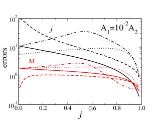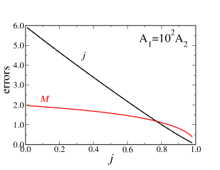
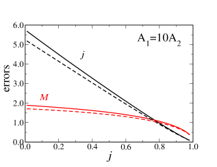
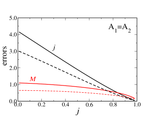
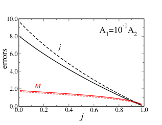
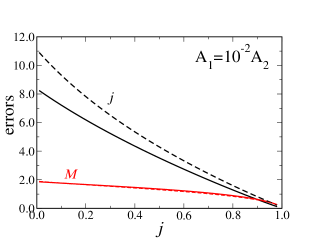
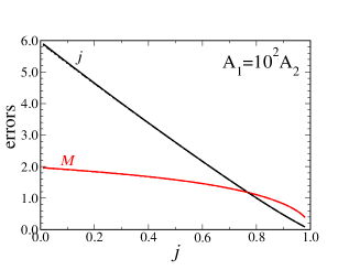
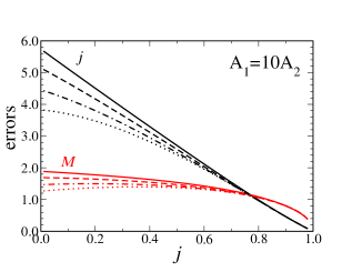
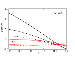
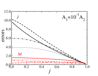
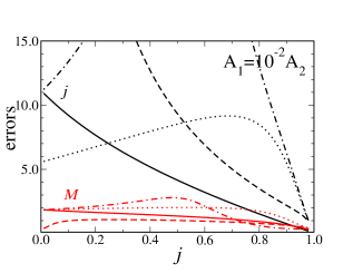
Secondly, we consider a more physically motivated case in which we fix $l=m=2$, $m^{\prime}=2$, so that both modes correspond to a “bar-shaped” deformation. We then look at the effect of setting $l^{\prime}=3,\,4$. Results for these combinations of angular indices are shown in Fig. 14. From left to right and from top to bottom we assume that the ratio of the two mode amplitudes ${\cal A}_{1}/{\cal A}_{2}=\left\{10^{2},~{}10,~{}1,~{}10^{-1},~{}10^{-2}\right\}$. Now the second mode plays some role, and we can observe a smooth deformation from the errors corresponding to $l=m=2$ (top left panel) to the errors corresponding to $l^{\prime}=3,~{}m^{\prime}=2$ or $l^{\prime}=4,~{}m^{\prime}=2$ (bottom right panel). Notice that the error on mass is roughly independent of $l$, but, when a single $l$ dominates, the error on angular momentum scales (roughly) as $l$. For $l=m=2$ the mass error becomes larger than the angular momentum error at $j\simeq 0.8$. As a consequence of the (rough) scaling with $l$ of $\rho\sigma_{j}$, this transition moves to larger and larger values of $j$ as the relative amplitude of the second mode grows. When $l^{\prime}=3$ dominates, the transition still occurs at $j\simeq 0.9$, but for $l^{\prime}=4$ the angular momentum error becomes subdominant (if at all) only for $j\gtrsim 0.95$.

In Fig. 14 we compute the derivatives $f_{lmn}^{\prime}$ and $Q_{lmn}^{\prime}$ “numerically” (that is, by local interpolating polynomials). However, we verified that the fits typically do a very good job, even though they are not as accurate as in the case considered above. This is expected, since we are considering corotating modes. For all of these modes $Q_{lmn}^{\prime}$ does not cross zero in the range $j\in[0,1]$ (see eg. Fig. 9), and the fits of Appendix E are reasonably accurate.

The third, and presumably the most physically realistic case, results from fixing $l=m=2$, $l^{\prime}=2$ and looking at the effect of changing $m^{\prime}$. In Fig. 15 we show the smooth deformation of the errors induced by changing ${\cal A}_{1}/{\cal A}_{2}$ in this case. Different linestyles correspond to $m^{\prime}=1,0,-1,-2$, as explained in the caption. The plot is better understood as a series of snapshots. The top left panel is an almost-pure $l=m=2$ waveform (closely approximating the top left panel of Fig. 12, or equivalently the left panel of Fig. 10). Each line becomes more and more dominated by the second mode, until (bottom right panels) it approximates quite closely the errors with $l=2$ and $m=1,0,-1,-2$ we displayed in Fig. 12. In the bottom right panels we clearly see signatures left by the dominance of the second mode. For example, the error becomes very large as $j\to 0$ for $m^{\prime}=0$, and as $j\to 0.6$ for $m^{\prime}=-1$.

In Fig. 15 the derivatives $f_{lmn}^{\prime}$ and $Q_{lmn}^{\prime}$ are computed numerically. The fits of Appendix E provide a good approximation of the numerical results, except for those cases (i.e. dominance of $m^{\prime}=0$ and $m^{\prime}=-1$) where the single-mode fits fail to reproduce the location of $Q_{lmn}^{\prime}=0$.

VI.2 Overtones with the same $l$ and $m$

Consider now modes for which $l=l^{\prime}$ and $m=m^{\prime}$. To reduce the number of parameters to be estimated, we assume that the plus- and cross-components have equal amplitudes (the generalization to unequal amplitudes is trivial). Approximating the scalar product between the different spin-weighted harmonics in this case by one, assuming that the frequencies are close enough that $S_{1}\simeq S_{2}\simeq S$, and using the expression (49) for the two-mode waveform, we get the following SNR:

$$\rho^{2}=\rho_{1}^{2}+\rho_{2}^{2}+\left(\frac{M}{r}\right)^{2}\frac{{\cal A}_{1}{\cal A}_{2}}{5\pi^{2}S}\left\{\frac{16f_{1}f_{2}Q_{1}^{3}Q_{2}^{3}(f_{1}Q_{2}+f_{2}Q_{1})\cos\phi}{\Lambda_{+}\Lambda_{-}}\right\}\,,$$ (53)

where

$$\Lambda_{\pm}=f_{2}^{2}Q_{1}^{2}+2f_{1}f_{2}Q_{1}Q_{2}+Q_{2}^{2}\left[f_{1}^{2}+4(f_{1}\pm f_{2})^{2}Q_{1}^{2}\right]\,,$$ (54)

and $\rho_{1}$ and $\rho_{2}$ are defined by Eq. (52).

Figure 16: Modulation of the total SNR, Eq. (53), induced by the second overtone. We consider an $l=m=2$ perturbation and three different values of the angular momentum $j$ (solid lines: $j=0$, dashed lines: $j=0.8$, dot-dashed lines: $j=0.98$). For concreteness, we assume that the first overtone has an amplitude ${\cal A}_{2}=10^{-1}{\cal A}_{1}$. The nearly horizontal (red) lines correspond to the SNR in the absence of modulations, Eq. (51).

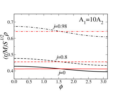
Fig. 16 shows a rescaled SNR given by $(r/M)S^{1/2}\rho$ as a function of $\phi$ for a reasonable amplitude ratio ${\cal A}_{2}/{\cal A}_{1}=10^{-1}$. The modulation induced by the mixed term is modest, and it scales (roughly) like $\left({\cal A}_{2}/{\cal A}_{1}\right)^{1/2}$.

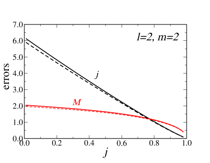
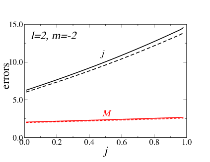
In Fig. 17 we compute the errors on mass and angular momentum for a two-mode waveform with ${\cal A}_{1}=10{\cal A}_{2}$, and compare the results with a single-mode waveform. We show two representative cases ($l=2,~{}m=2$ and $l=2,~{}m=-2$) but we looked at all modes with $l=2,~{}3,~{}4$ and all possible values of $m$. We always found that the correction induced by the addition of the second overtone is very small. Indeed, it is so small that it is comparable to the variations induced by different prescriptions to compute the error (compare the left panel with the left panel of Fig. 10).

A more realistic treatment would not assume that the second mode has amplitude 1/10 of the first, but would attempt to account for the mode excitation using an explicit calculation of the excitations coefficients as functions of $j$. We are currently working on such an approach.

Figure 17: Scaled errors ($\rho\sigma_{M}$, $\rho\sigma_{j}$) for the two-mode waveform (solid lines) versus a one-mode waveform (dashed line). Here we assume ${\cal A}_{1}=10{\cal A}_{2}$ and consider perturbations with $l=m=2$ (left) and $l=2$, $m=-2$ (right).

VII Resolving quasi-normal modes: critical signal-to-noise ratio to test the no-hair theorem

So far we have been discussing multi-mode detection without considering whether a discrimination between two different frequencies (in a signal buried in noise) is possible or not. A common rule of thumb to resolve the frequencies of two sinusoidal signals with equal amplitudes and quality factors is the so-called Rayleigh criterion (see eg. rayleigh ): two frequencies $f_{1}\,,\,f_{2}$ are resolvable if

$$|f_{1}-f_{2}|\Delta t>1\,,$$ (55)

where $\Delta t$ is the duration of the signal. This (purely classical) Rayleigh limit can be beaten, given a signal with sufficiently large SNR, as discussed in smilanfar ; milanfars . Here we introduce a slightly different resolvability criterion that allows for different amplitudes (${\cal A}_{1}\neq{\cal A}_{2}$) and quality factors ($Q_{1}\neq Q_{2}$). In Appendix D we will show that smilanfar ; milanfars actually deal with a very special case of our own resolvability criterion.

To determine whether two quasi-normal mode frequencies are resolvable we first need to determine the measurement errors. Here we work in terms of frequency and damping time, instead of $M$ and $j$. Because $Q_{lmn}=\pi f_{lmn}\tau_{lmn}$, the Fisher matrix in terms of $\tau_{lmn}$ may be written, for each index $k$, $\Gamma_{k\,\tau_{lmn}}=\pi f_{lmn}\Gamma_{k\,Q_{lmn}}$ and $\Gamma_{k\,f_{lmn}}=\Gamma_{k\,f_{lmn}}+\pi\tau_{lmn}\Gamma_{k\,Q_{lmn}}$. Inverting this Fisher matrix, one can show that the errors in $f_{lmn}$ and $\tau_{lmn}$ are given, to leading order for large Q, by

$$\sigma_{f}\simeq\frac{1}{\sqrt{2}\pi\tau\rho}\,,\qquad\sigma_{\tau}\simeq\frac{2\tau}{\rho}\,.$$ (56)

These relations reproduce to leading-order the large-$Q$ behavior predicted by Refs. finn ; kaa (which use a different parametrization of the waveform), except for a factor $\sqrt{2}$ in the leading term of $\sigma_{f}$.

Then, for detection of two modes, a natural criterion (á la Rayleigh) to resolve frequencies and damping times is

$$|f_{1}-f_{2}|>{\rm max}(\sigma_{f_{1}},\sigma_{f_{2}})\,,\qquad|\tau_{1}-\tau_{2}|>{\rm max}(\sigma_{\tau_{1}},\sigma_{\tau_{2}})\,.$$ (57)

This means, for example, that the frequencies are (barely) resolvable if “the maximum of the diffraction pattern of object 1 is located at the minimum of the diffraction pattern of object 2”. In other words, given two Gaussians with variance $\sigma$ we can only distinguish between the peaks if they are separated by a distance larger than $\sigma$. We can introduce two “critical” SNRs required to resolve frequencies and damping times,

$$\rho_{\rm crit}^{f} = \frac{{\rm max}(\rho\sigma_{f_{1}},\rho\sigma_{f_{2}})}{|f_{1}-f_{2}|}\,,$$ (58a)

$$\rho_{\rm crit}^{\tau} = \frac{{\rm max}(\rho\sigma_{\tau_{1}},\rho\sigma_{\tau_{2}})}{|\tau_{1}-\tau_{2}|}\,,$$ (58b)

and recast our resolvability conditions as

$$\rho > \rho_{\rm crit}={\rm min}(\rho_{\rm crit}^{f},\rho_{\rm crit}^{\tau})\,,$$ (59a)

$$\rho > \rho_{\rm both}={\rm max}(\rho_{\rm crit}^{f},\rho_{\rm crit}^{\tau})\,.$$ (59b)

The first condition implies resolvability of either the frequency or the damping time, the second implies resolvability of both.

We now need to compute the errors on frequencies ($\sigma_{f_{1}},~{}\sigma_{f_{2}}$) and damping times ($\sigma_{\tau_{1}},~{}\sigma_{\tau_{2}}$) in a two-mode situation. We again use the Fisher matrix formalism.

We first consider the waveform (49) in the quasi-orthonormal case of Sec. VI.1, and for simplicity we also pick $\phi=0$. Then the analytic expressions for the errors turn out to be very simple:

$$\rho\sigma_{f_{1}} = \frac{1}{2\sqrt{2}}\left\{\frac{f_{1}^{3}\left(3+16Q_{1}^{4}\right)}{{\cal A}_{1}^{2}Q_{1}^{7}}\left[\frac{{\cal A}_{1}^{2}Q_{1}^{3}}{f_{1}\left(1+4Q_{1}^{2}\right)}+\frac{{\cal A}_{2}^{2}Q_{2}^{3}}{f_{2}\left(1+4Q_{2}^{2}\right)}\right]\right\}^{1/2}\,,$$ (60a)

$$\rho\sigma_{\tau_{1}} = \frac{2}{\pi}\left\{\frac{\left(3+4Q_{1}^{2}\right)}{{\cal A}_{1}^{2}f_{1}Q_{1}}\left[\frac{{\cal A}_{1}^{2}Q_{1}^{3}}{f_{1}\left(1+4Q_{1}^{2}\right)}+\frac{{\cal A}_{2}^{2}Q_{2}^{3}}{f_{2}\left(1+4Q_{2}^{2}\right)}\right]\right\}^{1/2}\,.$$ (60b)

Since we consider the “symmetric” case $\phi=0$, the errors on $f_{2}$ and $\tau_{2}$ are simply obtained by exchanging indices ($1\leftrightarrow 2$). Notice also that the term in square parentheses is nothing but $5\pi^{2}S(r/M)^{2}\rho^{2}$, with $\rho^{2}$ given by Eq. (51). In the single-mode (${\cal A}_{2}\to 0$), large-$Q$ limit, these errors reproduce Eq. (56).

Figure 18: “Critical” SNR $\rho_{\rm crit}$ (top) and $\rho_{\rm both}$ (bottom) required to resolve different combinations of modes. Here we consider the “quasi-orthonormal” perturbations of Sec. VI.1 (either $l\neq l^{\prime}$ or $m\neq m^{\prime}$). Following the treatment in that Section, we always assume $l=m=2$ for the first mode. Different colors/linestyles refer to different values of $l^{\prime}$ and $m^{\prime}$ for the second mode. Black: $l^{\prime}=2$ and $m^{\prime}=1$ (solid), $m^{\prime}=0$ (dotted), $m^{\prime}=-1,~{}-2$ (dashed, top to bottom). Blue: $l^{\prime}=3$ and $m^{\prime}=2$ (solid), $m^{\prime}=3$ (dot-dashed). Red: $l^{\prime}=4$ and $m^{\prime}=2$ (solid), $m^{\prime}=4$ (dot-dashed). Different panels refer to different ratios ${\cal A}_{1}/{\cal A}_{2}$, as indicated.

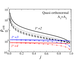
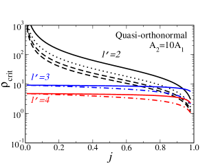
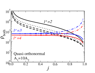
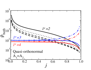
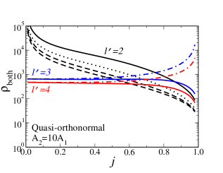A calculation of the critical SNRs $\rho_{\rm crit}$ and $\rho_{\rm both}$ for different QNM pairs is shown in Fig. 18. Most qualitative features of this plot can be explained by looking at Fig. 5. First, it is natural that modes with $l=l^{\prime}=2$ are harder to resolve than modes with $l^{\prime}\neq l$: in the latter case both frequencies and damping times are different. For the same reason, modes with $l=l^{\prime}$ and $m\simeq m^{\prime}$ are harder to resolve. Another predictable feature is that, for modes with $l=l^{\prime}$, the Schwarzschild limit is very bad in terms of resolvability: as $j\to 0$ all frequencies and damping times are degenerate with respect to $m$, so $\rho_{\rm crit}$ blows up. In particular, if modes with $l=2,~{}m=2$ and $l=2,~{}m=0$ are dominant (as suggested in fhh ), resolving them requires large SNRs for black holes with spin $j\lesssim 0.5$, especially if the amplitude ratio ${\cal A}_{1}/{\cal A}_{2}$ is not close to unity. The almost-flat $j$-dependence of $\rho_{\rm crit}$ and $\rho_{\rm both}$ for modes with $m^{\prime}=2$, $l^{\prime}=3,~{}4$ and $l^{\prime}=m^{\prime}=3,~{}4$ is in line with the corresponding discussion in Sec. VI.1: the errors on these modes have a very similar functional dependence on $j$, whatever the value of $l$ (or $m$), so it is natural for the critical SNR to be quite insensitive to $j$. As a rule of thumb, a large rotation parameter $j$ usually helps to resolve modes, mainly because of the larger quality factor (remember that we chose the first mode in the pair to have $l=m=2$). The only exception to this rule is the growth of $\rho_{\rm both}$ as $j\to 1$ for modes with $l=m=2$ and $l^{\prime}=m^{\prime}$($=3,4$). This growth is easy to understand: for all modes with $l=m$ the damping tends to zero in the extremal limit, so the denominator of Eq. (58b) goes to zero and the corresponding critical SNR blows up.

We now consider the resolvability of two overtones of modes with the same $l$ and $m$. Here an explicit calculation of the errors on frequency and damping time is not simple, because of the presence of “cross-terms” in the inner products. The final expressions are much more lengthy and involved than Eq. (60), so we do not include them here. Instead we carried out the calculation of Eqs. (58a)-(59b) numerically. We assumed that the waveform is a superposition of the fundamental mode and the first overtone with some given values of $(l,m)$, and made the plausible educated guess that the amplitude of the overtone is a factor ten smaller than the amplitude of the fundamental mode (${\cal A}_{1}=10{\cal A}_{2}$), meaning that the energy carried by the first overtone is roughly $1\%$ of the total energy radiated in the ringdown.

Our results for $\rho_{\rm crit}$ and $\rho_{\rm both}$ are shown in Figs. 3 and 4, respectively. Once again, most features of these plots can be explained by looking at Fig. 5. As long as we are content with resolving either the frequency or the damping time, higher $l$’s and positive $m$’s are easier to resolve because the frequency separations are similar, but the quality factor is larger. In fact, as $j$ grows the quality factor for corotating modes grows, but it decreases for counterrotating modes, and this affects resolvability in the corresponding way. If we want to distinguish both frequency and damping time, the behavior of the critical SNR changes. The corotating fundamental mode with $l=m$ is impossible to resolve from the first overtone in the extremal limit $j\to 1$ because they become degenerate, tending to the Detweiler frequency.

Fig. 3 shows that, quite independently of $(l,~{}m)$ and of the angular momentum $j$, resolving either the frequency or the damping time requires a SNR $\rho>\rho_{\rm crit}\sim 10^{2}$. Since the addition of a small-amplitude overtone does not significantly alter the SNR, we can use the SNR predictions of Fig. 7 to deduce that tests of the no-hair theorem should be feasible even under the most pessimistic assumptions on the ringdown efficiency $\epsilon_{\rm rd}$ (at least for equal-mass mergers) as long as the first overtone radiates a fraction $\sim 10^{-2}$ of the total ringdown energy. However, resolving both frequencies and damping times typically requires a SNR $\rho>\rho_{\rm both}\sim 10^{3}$. This is only possible under rather optimistic assumptions on the radiative efficiency, and it can be impossible if the dominant mode has $l=m=2$ and the black hole is rapidly spinning (solid black line in the left panel of Fig. 4). We hope to refine this analysis using computed estimates of excitation coefficients.

VIII Conclusions

We have presented a general framework for analysing the detectability of quasi-normal ringdown gravitational waves from massive black holes, and for using them to estimate parameters of the hole and to test the general relativistic no-hair theorem. In this initial work, we made a number of simplifying assumptions, including the reality of the spin-weighted spheroidal harmonics (thus simplifying the angle averaging), the restriction to one-mode or two-mode situations, and the assumption of large quality factors in deriving analytic expressions. In future work, we hope to explore the consequences of relaxing some of these assumptions. Although we focused on detection of modes using LISA, our framework is equally applicable to ground-based interferometers.

For example, the non-angle-averaged case can be studied using Monte Carlo simulations in place of angle averaging, thereby permitting inclusion of the fully complex spheroidal harmonics. Multi-mode calculations involving more than two modes should be carried out. Our discussion of testing the no-hair theorem has focused only on resolvability of modes; we hope to use our tools to perform in detail the no-hair test suggested in dreyer . A crucial point is to determine the excitation of modes. When they have different angular dependence, we must use numerical relativistic simulations of mergers, or minimally simulations of distorted black holes with initial data that mimics the merger. For overtones with the same angular dependence, we can use perturbative and analytical techniques to estimate the relative amplitudes; this work is in progress.

It will be important to extend the analysis from matched-filtering to more sophisticated data-analysis techniques (eg. the tiling method used by the TAMA group nakano ; tsunesada ) and combine them with time-delay interferometry (TDI), especially in the case of short damping times.

Another important question is the effect of combining parameter estimation from ringdown with parameter estimation from inspiral. This may make it possible to improve the measurement of mass or angular momentum by taking advantage of “prior” information, and may permit one to deduce how much energy and angular momentum is radiated in the merger phase.

Appendix A Accuracy of the $\delta$-function approximation

Figure 19: Modulus of the error in the SNR due to the $\delta$-function approximation, $|(\rho_{\delta}-\rho_{\rm{exact}})/\rho_{\rm{exact}}|$, for modes with $l=2$ and $l=4$, for $j=0.98$ and $D_{L}=3$ Gpc. For each $l$ we consider the fundamental mode ($n=0$) and the second overtone ($n=2$). The horizontal line marks a $10\%$ deviation from the “exact” result: for those modes lying below the horizontal line the $\delta$-function approximation can be considered very accurate. The “inverted peaks” are just zero-crossings of $|(\rho_{\delta}-\rho_{\rm{exact}})/\rho_{\rm{exact}}|$.

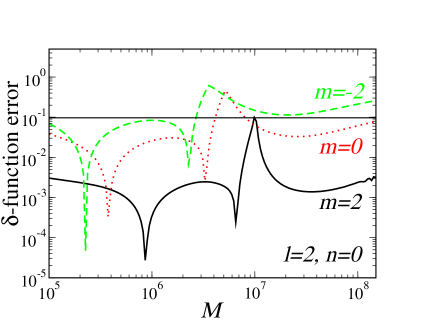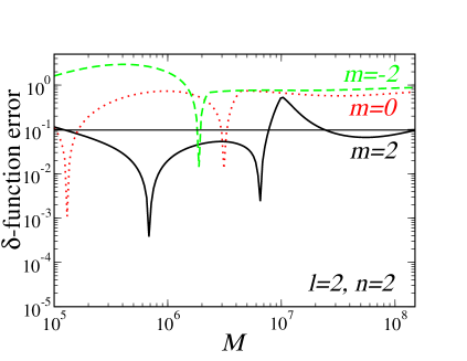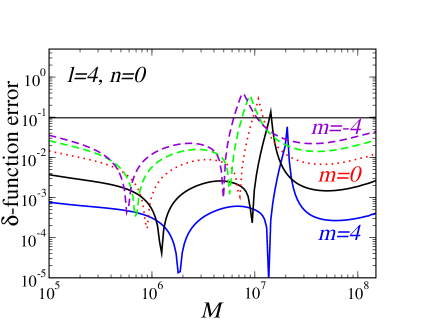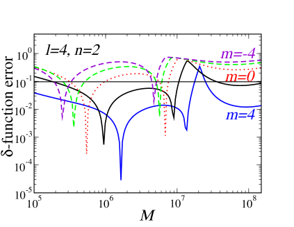How accurate is the $\delta$-function approximation we employed in Sec. III.1? The answer to this question depends on $(l,m,n)$ and on the angular momentum $j$ of the black hole. In general, we expect the approximation to hold better in the high-$Q_{lmn}$ limit: that is, for low overtones and (when the black hole is spinning) for modes with $m>0$. This expectation is made more quantitative in Fig. 19, where we plot the relative error on the SNR due to the $\delta$-function approximation for different modes as a function of the black hole mass, for $D_{L}=3$ Gpc. To compute the “exact” SNR, we use the FH SNR in the Breit-Wigner form [Eq. (18) or (21a)]. The plot refers to a near-extremal black hole ($j=0.98$), but the qualitative features we observe would be the same for different (non-zero) values of the rotation rate. In this near-extremal case the numerical integration of the “full” SNR becomes problematic for corotating modes ($m>0$), because the Breit-Wigner function effectively approaches a $\delta$-function. This problem usually shows up for very large masses (this is the origin of the small wiggles in the high-mass tail of the curve marked by $m=2$ in the top-left panel). To achieve some required numerical accuracy it is sufficient to double the number of integration points until the high-mass wiggles disappear and the integration routine converges.

The plot confirms our expectations. As a general trend, the $\delta$-function approximation is more accurate for corotating modes ($m>0$), for the simple reason that the quality factor $Q_{lmn}$ of corotating modes tends to infinity (or becomes very large) as $j\to 1$. The approximation is more accurate for slowly damped modes (small values of the overtone index $n$), which have a larger quality factor. As a rule of thumb, we can say that the $\delta$-function approximation is reasonably accurate whenever it induces deviations smaller than $\sim 10\%$ with respect to the exact result: all modes lying below the horizontal lines in Fig. 19 satisfy this criterion. Fig. 19 shows that the approximation is very accurate for the fundamental ($n=0$) mode, whatever the values of $(l,m)$. However, when we consider the $n=2$ overtone, it is only marginally accurate for corotating modes, and inaccurate for modes with $m\leq 0$.

The large deviation at mass $M\sim 10^{7}M_{\odot}$ corresponds to the frequency band where white-dwarf confusion noise dominates over instrumental noise. In this frequency band the noise curve is not a very smooth function, and the SNR (especially for corotating modes) is more sensitive to the “full” shape of the noise curve. We verified that the peak disappears when we omit the white-dwarf confusion noise from the Barack-Cutler noise curve. The larger disagreement in this frequency regime corresponds, unfortunately, to the most promising mass range for detection of black hole ringdown from galactic centers. This means that we probably need a good control of the white-dwarf confusion noise (and a rather accurate model of the ringdown waveform) to detect these events.

Appendix B Fisher matrices for a single-mode waveform

Taking the Fourier transform of ringdown waveforms requires some care. For ringdown waves from SMBH mergers, the waveform emitted before ringdown starts (say, for $t<0$) is the poorly known merger waveform. To obtain the SNR from the ringdown signal alone, a possible guess is to assume that the waveform $h(t)=0$ for $t<0$. Under this assumption we can calculate the Fourier transform of the waveform by integrating only over the range $t>0$. This method was used, among others, by Echeverria echeverria and Finn finn , and for this reason we call it the Echeverria-Finn (EF) convention. More rigorously, we would really like to know the probability that a ringdown waveform is present in the data stream starting (say) at $t=0$. This probability should be computed integrating over all possible realizations of the noise for $t<0$. Appendix A of FH shows that this is equivalent to minimizing the SNR over all choices of the function $h(t)$ on the negative $t$ axis, and that the SNR obtained by minimizing over these choices is always within a few tens of a percent of the SNR obtained using the “FH prescription”, as described in Section III.1. In the body of the paper we usually adopt the FH prescription. In this Appendix we present, for completeness, the Fisher matrix calculation in the EF convention. We also list the elements of the Fisher matrix adopting the FH convention, but assuming that we do not know a priori the relative amplitudes or phases of the two polarizations.

B.1 Echeverria-Finn convention, four parameters

Here we compute the single-mode Fisher matrix following the Echeverria-Finn convention for calculating the Fourier transforms. We start with the waveform as defined in Eqs. (38) – (40). But in this case, instead of taking $|t|$ in the damped exponential, integrating over $t$ from $-\infty$ to $+\infty$ and dividing the resulting spectrum by $\sqrt{2}$ to compensate for the doubling, we assume that the waveform vanishes for $t<0$, and integrate only over positive $t$.

Assuming that the noise can be considered constant over the bandwidth of the signal, we get the angle-averaged SNR $\rho_{\rm EF}=\gamma(1+4Q_{lmn}^{2}-\beta+2Q_{lmn}\alpha)$, where $\alpha$, $\beta$ and $\gamma$ are given by Eqs. (42). The result is equivalent to Eq. (32).

The Fisher matrix in the $(A^{+},\,\phi_{lmn}^{+},\,f_{lmn},\,Q_{lmn})$ basis is given by

$$\Gamma_{A^{+}A^{+}} = \frac{\gamma}{(A^{+})^{2}}\left(1+4Q_{lmn}^{2}-\beta+2Q_{lmn}\alpha\right)\,,$$ (61a)

$$\Gamma_{A^{+}\phi_{lmn}^{+}} = \frac{\gamma}{A^{+}}\left(\alpha+2Q_{lmn}\beta\right)\,,$$ (61b)

$$\Gamma_{A^{+}f_{lmn}} = -\frac{\gamma}{2A^{+}f_{lmn}}\left(1+4Q_{lmn}^{2}-\beta+2Q_{lmn}\alpha\right)\,,$$ (61c)

$$\Gamma_{A^{+}Q_{lmn}} = \frac{\gamma}{2A^{+}Q_{lmn}}\frac{1}{1+4Q_{lmn}^{2}}\left[(1+4Q_{lmn}^{2})^{2}-(1-4Q_{lmn}^{2})\beta+4Q_{lmn}\alpha\right]\,,$$ (61d)

$$\Gamma_{\phi_{lmn}^{+}\phi_{lmn}^{+}} = \gamma\left(1+4Q_{lmn}^{2}+\beta-2Q_{lmn}\alpha\right)\,,$$ (61e)

$$\Gamma_{\phi_{lmn}^{+}f_{lmn}} = -\frac{\gamma}{2f_{lmn}}\left[\alpha-2Q_{lmn}(1+4Q_{lmn}^{2}-\beta)\right]\,,$$ (61f)

$$\Gamma_{\phi_{lmn}^{+}Q_{lmn}} = \frac{\gamma}{2Q_{lmn}}\left(\frac{1}{1+4Q_{lmn}^{2}}\right)\left[(1-4Q_{lmn}^{2})\alpha+4Q_{lmn}\beta\right]\,,$$ (61g)

$$\Gamma_{f_{lmn}f_{lmn}} = \frac{\gamma}{2f_{lmn}^{2}}\left[(1+4Q_{lmn}^{2})^{2}-\beta+2Q_{lmn}\alpha\right]\,,$$ (61h)

$$\Gamma_{f_{lmn}Q_{lmn}} = -\frac{\gamma}{2f_{lmn}Q_{lmn}}\frac{1}{1+4Q_{lmn}^{2}}\left[(1+4Q_{lmn}^{2})^{2}-(1-4Q_{lmn}^{2})\beta+4Q_{lmn}\alpha\right]\,,$$ (61i)

$$\Gamma_{Q_{lmn}Q_{lmn}} = \frac{\gamma}{2Q_{lmn}^{2}}\frac{1}{(1+4Q_{lmn}^{2})^{2}}\left[(1+4Q_{lmn}^{2})^{3}-(1-12Q_{lmn}^{2})\beta+(6-8Q_{lmn}^{2})Q_{lmn}\alpha\right]\,.$$ (61j)

In the $(A^{+},\,\phi_{lmn}^{+},\,M,\,j)$ basis, an expansion of the errors in powers of $Q_{lmn}^{-1}$ gives

$$\sigma_{j} = \frac{1}{\rho_{\rm EF}}\left|2\frac{Q_{lmn}}{Q_{lmn}^{\prime}}\left(1+\frac{1+\alpha^{2}+2\beta^{2}}{8Q_{lmn}^{2}}\right)\right|\,,$$ (62a)

$$\sigma_{M} = \frac{1}{\rho_{\rm EF}}\left|2\frac{MQ_{lmn}f_{lmn}^{\prime}}{f_{lmn}Q_{lmn}^{\prime}}\left(1+\frac{1+\alpha^{2}+2\beta^{2}}{8Q_{lmn}^{2}}\right)\right|\,,$$ (62b)

$$\sigma_{A^{+}} = \frac{\sqrt{2}A^{+}}{\rho_{\rm EF}}\left|1-\frac{\alpha}{4Q_{lmn}}\right|\,,$$ (62c)

$$\sigma_{\phi_{lmn}^{+}} = \frac{\sqrt{2}}{\rho_{\rm EF}}\left|1+\frac{3\alpha}{4Q_{lmn}}\right|\,.$$ (62d)

For the correlation coefficients we get

$$r_{jM} = {\rm sgn}(f_{lmn}^{\prime})\times\left(1-\frac{f_{lmn}^{2}Q_{lmn}^{\prime 2}}{8f_{lmn}^{\prime 2}Q_{lmn}^{4}}\right)+{\cal O}(1/Q^{5})\,,$$ (63a)

$$r_{jA} = -\frac{1}{\sqrt{2}}\left(1-\frac{\alpha}{4Q_{lmn}}\right)+{\cal O}(1/Q^{2})\,,$$ (63b)

$$r_{MA} = -\frac{1}{\sqrt{2}}\left(1-\frac{\alpha}{4Q_{lmn}}\right)+{\cal O}(1/Q^{2})\,,$$ (63c)

$$r_{j\phi_{lmn}^{+}} = -\frac{1}{2\sqrt{2}}\frac{1-2\beta}{Q_{lmn}}+{\cal O}(1/Q^{2})\,,$$ (63d)

$$r_{M\phi_{lmn}^{+}} = -\frac{1}{2\sqrt{2}}\frac{1-2\beta}{Q_{lmn}}+{\cal O}(1/Q^{2})\,,$$ (63e)

$$r_{A\phi_{lmn}^{+}} = -\frac{\beta}{Q_{lmn}}-\frac{\alpha}{Q_{lmn}^{2}}+{\cal O}(1/Q^{3})\,.$$ (63f)

B.2 Flanagan-Hughes convention, six parameters

Here we list the elements of the Fisher matrix for the case where we do not know a priori the relative amplitudes or phases of the two polarizations. In the six-parameter basis $(A^{+},\,A^{\times},\,\phi_{lmn}^{+},\,\phi_{lmn}^{\times},\,f_{lmn},\,Q_{lmn})$, they are

$$\Gamma_{A^{+}A^{+}} = \frac{\gamma}{A^{2}}\left(1+4Q_{lmn}^{2}+\cos 2\phi_{lmn}^{+}\right)\,,$$ (64a)

$$\Gamma_{A^{\times}A^{\times}} = \frac{\gamma}{A^{2}}\left(1+4Q_{lmn}^{2}\ -\cos 2\phi_{lmn}^{\times}\right)\,,$$ (64b)

$$\Gamma_{A^{+}A^{\times}} = \Gamma_{A^{+}\phi_{lmn}^{\times}}=\Gamma_{A^{\times}\phi_{lmn}^{+}}=0\,,$$ (64c)

$$\Gamma_{A^{+}\phi_{lmn}^{+}} = -\frac{\gamma}{A}\sin 2\phi_{lmn}^{+}\cos\psi\,,$$ (64d)

$$\Gamma_{A^{\times}\phi_{lmn}^{\times}} = \frac{\gamma}{A}\sin 2\phi_{lmn}^{\times}\sin\psi\,,$$ (64e)

$$\Gamma_{A^{+}f_{lmn}} = -\frac{\gamma}{2Af_{lmn}}\left(1+4Q_{lmn}^{2}+\cos 2\phi_{lmn}^{+}\right)\cos\psi\,,$$ (64f)

$$\Gamma_{A^{\times}f_{lmn}} = -\frac{\gamma}{2Af_{lmn}}\left(1+4Q_{lmn}^{2}-\cos 2\phi_{lmn}^{\times}\right)\sin\psi\,,$$ (64g)

$$\Gamma_{A^{+}Q_{lmn}} = \frac{\gamma}{2AQ_{lmn}}\frac{1}{1+4Q_{lmn}^{2}}\left[(1+4Q_{lmn}^{2})^{2}+(1-4Q_{lmn}^{2})\cos 2\phi_{lmn}^{+}\right]\cos\psi\,,$$ (64h)

$$\Gamma_{A^{\times}Q_{lmn}} = \frac{\gamma}{2AQ_{lmn}}\frac{1}{1+4Q_{lmn}^{2}}\left[(1+4Q_{lmn}^{2})^{2}-(1-4Q_{lmn}^{2})\cos 2\phi_{lmn}^{\times}\right]\sin\psi\,,$$ (64i)

$$\Gamma_{\phi_{lmn}^{+}\phi_{lmn}^{+}} = \gamma\left(1+4Q_{lmn}^{2}-\cos 2\phi^{+}\right)\cos^{2}\psi\,,$$ (64j)

$$\Gamma_{\phi_{lmn}^{\times}\phi_{lmn}^{\times}} = \gamma\left(1+4Q_{lmn}^{2}+\cos 2\phi^{\times}\right)\sin^{2}\psi\,,$$ (64k)

$$\Gamma_{\phi_{lmn}^{+}\phi_{lmn}^{\times}} = 0\,,$$ (64l)

$$\Gamma_{\phi_{lmn}^{+}f_{lmn}} = \frac{\gamma}{2f_{lmn}}\sin 2\phi_{lmn}^{+}\cos^{2}\psi\,,$$ (64m)

$$\Gamma_{\phi_{lmn}^{\times}f_{lmn}} = -\frac{\gamma}{2f_{lmn}}\sin 2\phi_{lmn}^{\times}\sin^{2}\psi\,,$$ (64n)

$$\Gamma_{\phi_{lmn}^{+}Q_{lmn}} = -\frac{\gamma}{2Q_{lmn}}\left(\frac{1-4Q_{lmn}^{2}}{1+4Q_{lmn}^{2}}\right)\sin 2\phi^{+}\cos^{2}\psi\,,$$ (64o)

$$\Gamma_{\phi_{lmn}^{\times}Q_{lmn}} = \frac{\gamma}{2Q_{lmn}}\left(\frac{1-4Q_{lmn}^{2}}{1+4Q_{lmn}^{2}}\right)\sin 2\phi^{\times}\sin^{2}\psi\,,$$ (64p)

$$\Gamma_{f_{lmn}f_{lmn}} = \frac{\gamma}{2f_{lmn}^{2}}\left[(1+4Q_{lmn}^{2})^{2}-\beta\right]\,,$$ (64q)

$$\Gamma_{f_{lmn}Q_{lmn}} = -\frac{\gamma}{2f_{lmn}Q_{lmn}}\frac{1}{1+4Q_{lmn}^{2}}\left[(1+4Q_{lmn}^{2})^{2}-(1-4Q_{lmn}^{2})\beta\right]\,,$$ (64r)

$$\Gamma_{Q_{lmn}Q_{lmn}} = \frac{\gamma}{2Q_{lmn}^{2}}\frac{1}{(1+4Q_{lmn}^{2})^{2}}\left[(1+4Q_{lmn}^{2})^{3}-(1-12Q_{lmn}^{2})\beta\right]\,,$$ (64s)

where $A^{2}=(A^{+})^{2}+(A^{\times})^{2}$, $\cos\psi\equiv A^{+}/A$ and $\sin\psi\equiv A^{\times}/A$, and where $\alpha$, $\beta$ and $\gamma$ are given by Eqs. (42). Also, as in the four-parameter case, $\rho_{FH}^{2}=\gamma(1+4Q_{lmn}^{2}-\beta)$.

As before, one can convert to the $(M,j)$ basis using Eqs. (43), and then invert the Fisher matrix to obtain the errors and correlation coefficients. The resulting formulae are lengthy and unenlightening, and we do not display them here.

Appendix C LISA noise curve

Generally, the LISA  community has been using the so-called sky-averaged spectral noise density $S_{h}^{\rm SA}$ [see e.g., Ref. FT and the LISA Pre-Phase A Report], computed by a combination of three factors, including: (i) the raw spectral noise density $S_{n}$, (ii) the gravitational-wave transfer (response) function $R$ and (iii) the noise transfer (response) function $R_{n}$. They combine together in LHH

$$S_{h}^{\rm SA}=\frac{S_{n}\,R_{n}}{R}\,.$$ (65)

In the low frequency limit, the GW transfer function used in the LISA Sensitivity Curve Generator SCG is $R=4(\sqrt{3}/2)^{2}1/5=3/5$, where the factor $(\sqrt{3}/2)^{2}$ comes from the LISA arms being at $60^{o}$, the factor 1/5 is due to the sky-average of the pattern functions ($\langle F_{+,\times}^{2}\rangle=1/5$) and the factor 4 depends on the particular read-out variable used. Since our definition of the GW signal already includes the factor $\sqrt{3}/2$, and since we choose to sky-average the signal, we use an effective non-sky-averaged spectral density, obtained by multplying $S_{h}^{\rm SA}$ by $(\sqrt{3}/2)^{2}/5=3/20$. The final result is Eq. (29), and has been obtained also in Ref. BC . We estimate white-dwarf confusion noise following BC , which uses results from conf1 ; conf2 : the galactic contribution is approximated as

$$S_{h}^{\rm gal}(f)=2.1\times 10^{-45}\left(\frac{f}{1~{}{\rm Hz}}\right)^{-7/3}~{}{\rm Hz}^{-1}\,,$$ (66)

and the contribution from extra-galactic white dwarfs as

$$S_{h}^{\rm ex-gal}(f)=4.2\times 10^{-47}\left(\frac{f}{1~{}{\rm Hz}}\right)^{-7/3}~{}{\rm Hz}^{-1}\,.$$ (67)

We compute the total (instrumental plus confusion) noise as

$$S_{h}(f)={\rm min}\left\{S_{h}^{\rm NSA}(f)/{\rm exp}\left(-\kappa T^{-1}_{\rm mission}dN/df\right),~{}S_{h}^{\rm NSA}(f)+S_{h}^{\rm gal}(f)\right\}+S_{h}^{\rm ex-gal}(f)\,.$$ (68)

Here $dN/df$ is the number density of galactic white-dwarf binaries per unit gravitational-wave frequency, for which we adopt the estimate

$$\frac{dN}{df}=2\times 10^{-3}~{}{\rm Hz}^{-1}\left(\frac{1~{}{\rm Hz}}{f}\right)^{11/3}\,;$$ (69)

$\Delta f=T^{-1}_{\rm mission}$ is the bin size of the discretely Fourier transformed data for a LISA mission lasting a time $T_{\rm mission}$; and $\kappa\simeq 4.5$ is the average number of frequency bins that are lost when each galactic binary is fitted out. The factor ${\rm exp}\left(-\kappa T^{-1}_{\rm mission}dN/df\right)$ thus represents the fraction of “uncorrupted” bins where instrumental noise still dominates. The analytic root noise spectral density curve (68) used in this paper is shown in Fig. 20 together with the corresponding root noise spectral density curve from the LISA Sensitivity Curve Generator SCG . The SCG curve shown is obtained using the nominal values SNR=1, arm length $=5\times 10^{9}$ m, telescope diameter $=0.3$ m, laser wavelength $=1064$ nanometers, laser power $=1.0$ Watts, optical train efficiency $=0.3$, acceleration noise $=3\times 10^{-15}\,{\rm m}\,{\rm s}^{-2}\,{\rm Hz}^{-1/2}$, and position noise budget $=2\times 10^{-11}\,{\rm m}\,{\rm Hz}^{-1/2}$, with position noise setting the floor at high frequency. The data returned by the SCG is then multiplied by $\sqrt{3/20}$ to obtain the effective non-sky averaged curve shown in Fig.  20.

Figure 20: Analytic approximation to the LISA  root noise spectral density curve used in this paper and in Ref. BC (dashed line) and the curve produced using the LISA Sensitivity Curve Generator SCG (solid line). The SCG curve has been multiplied by a factor of $\sqrt{3/20}$ to obtain an effective non-sky averaged noise spectral density. The SCG noise curve does not include the extragalactic white dwarf confusion noise while the analytical approximation curve does.

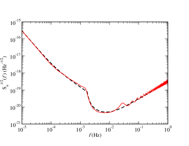
Appendix D The Shahram-Milanfar criterion for resolvability

For damped sinusoids it makes sense to assume that the signal duration $\Delta t$ is given by the e-folding time $\tau$, so the “standard” Rayleigh criterion (55) becomes $(f_{1}-f_{2})\tau>1$. In smilanfar (see also milanfars ) the authors discuss how to go beyond this (purely classical) Rayleigh limit. They show how to bypass this limit for two sinusoids with nearby frequencies $f_{1}\,,f_{2}$ such that $2\delta\equiv f_{1}-f_{2}\ll 1/B$, where $B$ is the duration of the signal. Assuming white noise with zero mean and unit variance $\sigma^{2}$, they get a condition for the minimum SNR required for the frequencies of two equal-amplitude sinusoids to be resolved notemilanfar :

$$\rho^{2}\geq\frac{640}{\pi^{4}}\frac{\left(T^{-1}(P_{f})-T^{-1}(P_{d})\right)^{2}}{(2\delta B)^{4}}\,.$$ (70)

Here $T(x)$ is the right-tail probability function for a Gaussian random variable $X$ with zero mean and unit variance noterighttail . $P_{d}$ and $P_{f}$ denote the detection and false-alarm rates, typical values for these being, say, $P_{d}=0.99\,,\,P_{f}=0.01$. Their analysis can be carried over to our case, assuming large $Q$ factors, and therefore a signal with duration $\tau\sim Q/f$. We would get

$$\rho^{2}\geq\frac{640}{\pi^{4}}\frac{\left(T^{-1}(P_{f})-T^{-1}(P_{d})\right)^{2}}{\tau^{4}(f_{1}-f_{2})^{4}}\sim\frac{1}{\tau^{4}(f_{1}-f_{2})^{4}}\,.$$ (71)

For overtones (“nearly-parallel signals”, in the sense of the scalar product of SWSHs being close to unity) with equal amplitudes and quality factors the frequency error has a large-$Q$ behavior

$$\sigma_{f}\sim\frac{1}{\rho\tau^{2}|f_{1}-f_{2}|}\,,$$ (72)

so our frequency resolvability criterion, $|f_{1}-f_{2}|>{\rm max}\left(\sigma_{f_{1}},\sigma_{f_{2}}\right)$ agrees with the Shahram-Milanfar result (71). Notice however that the situation considered in smilanfar is very special: overtones with the same $(l,m)$, equal amplitudes ${\cal A}_{1}={\cal A}_{2}$ and equal quality factors $Q_{1}=Q_{2}$ are the only class of modes for which $\sigma_{f}\sim 1/|f_{1}-f_{2}|$.

Appendix E Quasinormal frequencies for rotating black holes

There is a vast literature on Kerr QNMs leaver ; sai ; onozawa ; cardosoberti , but the QNM frequencies which are relevant for detection have never been systematically tabulated. Here we list for reference the values of the complex frequencies and separation constants for selected QNMs. These were calculated using two different numerical implementations of the continued fraction method of Leaver leaver , one written by one of us (EB), and the other provided by Hisashi Onozawa. Both methods give results in excellent agreement with each other. Shown in Tables 2, 3 and 4 are the real and imaginary parts of the complex QNM frequencies, separated by commas, for $l=2$, $3$ and $4$, respectively, and for the three lowest overtones. Tables 5, 6 and 7 display the angular separation constants $A_{lmn}$ in the same format. Following Leaver, the numerical values of the $A_{lmn}$’s were obtained assuming that the perturbations have a time dependence of the form $e^{-{\rm i}\omega t}$, while in this paper we use the opposite convention on the Fourier transform.

Table 2: First three overtones for $l=2$. A comma separates the real part from the imaginary part of $M\omega$. To save space, in this and the following Tables we omit leading zeros.

$l=2$, $n=0$
$j$	$m=2$	$m=1$	$m=0$	$m=-1$	$m=-2$
0.00	.3737,.0890	.3737,.0890	.3737,.0890	.3737,.0890	.3737,.0890
0.10	.3870,.0887	.3804,.0888	.3740,.0889	.3678,.0890	.3618,.0891
0.20	.4021,.0883	.3882,.0885	.3751,.0887	.3627,.0889	.3511,.0892
0.30	.4195,.0877	.3973,.0880	.3770,.0884	.3584,.0888	.3413,.0892
0.40	.4398,.0869	.4080,.0873	.3797,.0878	.3546,.0885	.3325,.0891
0.50	.4641,.0856	.4206,.0862	.3833,.0871	.3515,.0881	.3243,.0890
0.60	.4940,.0838	.4360,.0846	.3881,.0860	.3489,.0876	.3168,.0890
0.70	.5326,.0808	.4551,.0821	.3941,.0845	.3469,.0869	.3098,.0887
0.80	.5860,.0756	.4802,.0780	.4019,.0822	.3454,.0860	.3033,.0885
0.90	.6716,.0649	.5163,.0698	.4120,.0785	.3444,.0849	.2972,.0883
0.98	.8254,.0386	.5642,.0516	.4223,.0735	.3439,.0837	.2927-.0881
$l=2$, $n=1$
$j$	$m=2$	$m=1$	$m=0$	$m=-1$	$m=-2$
0.00	.3467,.2739	.3467,.2739	.3467,.2739	.3467,.2739	.3467,.2739
0.10	.3619,.2725	.3545,.2731	.3472,.2737	.3400,.2744	.3330,.2750
0.20	.3790,.2705	.3635,.2717	.3486,.2730	.3344,.2744	.3206,.2759
0.30	.3984,.2680	.3740,.2698	.3511,.2718	.3296,.2741	.3093,.2765
0.40	.4208,.2647	.3863,.2670	.3547,.2700	.3256,.2734	.2989,.2769
0.50	.4474,.2602	.4009,.2631	.3594,.2674	.3225,.2723	.2893,.2772
0.60	.4798,.2538	.4183,.2575	.3655,.2638	.3201,.2708	.2803,.2773
0.70	.5212,.2442	.4399,.2492	.3732,.2585	.3184,.2686	.2720,.2773
0.80	.5779,.2281	.4676,.2358	.3826,.2507	.3173,.2658	.2643,.2772
0.90	.6677,.1953	.5059,.2097	.3935,.2385	.3167,.2620	.2570,.2770
0.98	.8249,.1159	.5477,.1509	.4014,.2231	.3164,.2581	.2515,.2768
$l=2$, $n=2$
$j$	$m=2$	$m=1$	$m=0$	$m=-1$	$m=-2$
0.00	.3011,.4783	.3011,.4783	.3011,.4783	.3011,.4783	.3011,.4783
0.10	.3192,.4735	.3104,.4756	.3017,.4778	.2932,.4801	.2846,.4825
0.20	.3393,.4679	.3214,.4719	.3038,.4764	.2866,.4811	.2697,.4862
0.30	.3619,.4613	.3342,.4671	.3074,.4739	.2813,.4814	.2559,.4895
0.40	.3878,.4533	.3492,.4607	.3124,.4701	.2772,.4808	.2433,.4925
0.50	.4179,.4433	.3669,.4522	.3190,.4647	.2741,.4794	.2316,.4952
0.60	.4542,.4303	.3878,.4407	.3273,.4571	.2721,.4768	.2207,.4977
0.70	.4999,.4123	.4133,.4241	.3374,.4464	.2709,.4729	.2107,.4999
0.80	.5622,.3839	.4451,.3984	.3488,.4307	.2703,.4674	.2013,.5019
0.90	.6598,.3275	.4867,.3502	.3591,.4067	.2697,.4600	.1925,.5038
0.98	.8238,.1933	.5201,.2331	.3599,.3808	.2686,.4527	.1858,.5051

Table 3: First three overtones for $l=3$.

$l=3$, $n=0$
$j$	$m=3$	$m=2$	$m=1$	$m=0$	$m=-1$	$m=-2$	$m=-3$
0.00	.5994,.0927	.5994,.0927	.5994,.0927	.5994,.0927	.5994,.0927	.5994,.0927	.5994,.0927
0.10	.6208,.0924	.6137,.0925	.6067,.0926	.5999,.0926	.5932,.0927	.5867,.0928	.5802,.0928
0.20	.6448,.0920	.6297,.0921	.6153,.0923	.6014,.0924	.5880,.0926	.5752,.0927	.5628,.0929
0.30	.6721,.0913	.6480,.0915	.6252,.0918	.6038,.0921	.5837,.0923	.5647,.0926	.5469,.0928
0.40	.7037,.0902	.6689,.0906	.6369,.0911	.6074,.0915	.5802,.0920	.5553,.0924	.5323,.0927
0.50	.7409,.0887	.6934,.0893	.6506,.0900	.6121,.0908	.5776,.0915	.5467,.0920	.5188,.0925
0.60	.7862,.0864	.7228,.0873	.6670,.0885	.6183,.0897	.5758,.0908	.5388,.0916	.5063,.0922
0.70	.8437,.0829	.7592,.0842	.6870,.0861	.6261,.0882	.5749,.0899	.5316,.0912	.4946,.0919
0.80	.9219,.0770	.8068,.0791	.7121,.0824	.6360,.0860	.5749,.0888	.5250,.0906	.4837,.0916
0.90	1.0446,.0655	.8762,.0689	.7455,.0758	.6487,.0826	.5758,.0872	.5191,.0900	.4735,.0913
0.98	1.2602,.0387	.9769,.0453	.7833,.0643	.6615,.0782	.5773,.0856	.5146,.0894	.4657,.0910
$l=3$, $n=1$
$j$	$m=3$	$m=2$	$m=1$	$m=0$	$m=-1$	$m=-2$	$m=-3$
0.00	.5826,.2813	.5826,.2813	.5826,.2813	.5826,.2813	.5826,.2813	.5826,.2813	.5826,.2813
0.10	.6053,.2802	.5978,.2805	.5904,.2808	.5832,.2811	.5761,.2814	.5691,.2817	.5623,.2820
0.20	.6306,.2785	.6148,.2791	.5995,.2798	.5848,.2804	.5706,.2811	.5569,.2817	.5437,.2823
0.30	.6593,.2761	.6341,.2771	.6102,.2782	.5876,.2793	.5662,.2804	.5459,.2814	.5268,.2823
0.40	.6924,.2726	.6563,.2741	.6227,.2758	.5916,.2776	.5627,.2793	.5360,.2808	.5112,.2822
0.50	.7312,.2676	.6821,.2698	.6375,.2724	.5969,.2751	.5602,.2777	.5270,.2800	.4967,.2818
0.60	.7782,.2604	.7130,.2634	.6550,.2674	.6038,.2717	.5587,.2756	.5188,.2789	.4833,.2813
0.70	.8375,.2494	.7510,.2538	.6762,.2600	.6124,.2668	.5580,.2728	.5113,.2775	.4708,.2807
0.80	.9176,.2315	.8004,.2379	.7025,.2484	.6230,.2598	.5582,.2692	.5045,.2758	.4590,.2800
0.90	1.0425,.1966	.8714,.2068	.7362,.2277	.6357,.2491	.5593,.2644	.4983,.2739	.4480,.2792
0.98	1.2599,.1161	.9706,.1341	.7679,.1930	.6468,.2359	.5606,.2593	.4938,.2720	.4396,.2784
$l=3$, $n=2$
$j$	$m=3$	$m=2$	$m=1$	$m=0$	$m=-1$	$m=-2$	$m=-3$
0.00	.5517,.4791	.5517,.4791	.5517,.4791	.5517,.4791	.5517,.4791	.5517,.4791	.5517,.4791
0.10	.5766,.4763	.5684,.4771	.5603,.4779	.5523,.4787	.5445,.4795	.5368,.4803	.5292,.4812
0.20	.6043,.4725	.5872,.4741	.5705,.4758	.5543,.4775	.5386,.4792	.5234,.4809	.5086,.4826
0.30	.6356,.4674	.6084,.4699	.5825,.4725	.5577,.4753	.5340,.4781	.5114,.4809	.4897,.4836
0.40	.6714,.4605	.6328,.4640	.5966,.4679	.5625,.4721	.5305,.4763	.5005,.4804	.4723,.4842
0.50	.7131,.4511	.6612,.4558	.6131,.4614	.5689,.4675	.5282,.4736	.4907,.4793	.4561,.4845
0.60	.7632,.4379	.6948,.4441	.6327,.4522	.5769,.4611	.5270,.4698	.4819,.4778	.4410,.4846
0.70	.8258,.4185	.7358,.4268	.6561,.4387	.5868,.4521	.5267,.4648	.4739,.4757	.4269,.4843
0.80	.9096,.3874	.7884,.3988	.6844,.4177	.5984,.4391	.5272,.4581	.4667,.4730	.4136,.4839
0.90	1.0383,.3282	.8622,.3449	.7177,.3806	.6106,.4197	.5282,.4492	.4600,.4696	.4011,.4834
0.98	1.2592,.1935	.9605,.2181	.7349,.3224	.6176,.3976	.5286,.4403	.4550,.4665	.3916,.4828

Table 4: First three overtones for $l=4$.

$l=4$, $n=0$
$j$	$m=4$	$m=3$	$m=2$	$m=1$	$m=0$	$m=-1$	$m=-2$	$m=-3$	$m=-4$
0.00	.8092,.0942	.8092,.0942	.8092,.0941	.8092,.0942	.8092,.0942	.8092,.0942	.8092,.0942	.8092,.0942	.8092,.0942
0.10	.8387,.0940	.8313,.0940	.8240,.0940	.8168,.0941	.8098,.0941	.8028,.0941	.7960,.0942	.7893,.0942	.7826,.0942
0.20	.8717,.0935	.8560,.0936	.8407,.0937	.8259,.0938	.8116,.0939	.7977,.0940	.7842,.0941	.7712,.0941	.7585,.0942
0.30	.9092,.0929	.8839,.0930	.8597,.0932	.8366,.0934	.8146,.0935	.7937,.0937	.7737,.0938	.7546,.0940	.7365,.0941
0.40	.9525,.0918	.9159,.0921	.8815,.0924	.8493,.0927	.8191,.0930	.7908,.0933	.7643,.0935	.7395,.0937	.7162,.0939
0.50	1.0034,.0903	.9532,.0907	.9069,.0912	.8642,.0917	.8250,.0922	.7890,.0927	.7559,.0931	.7255,.0934	.6974,.0936
0.60	1.0650,.0879	.9978,.0885	.9369,.0893	.8820,.0902	.8326,.0911	.7883,.0919	.7485,.0925	.7125,.0930	.6800,.0933
0.70	1.1427,.0842	1.0530,.0852	.9734,.0865	.9035,.0881	.8423,.0896	.7889,.0909	.7420,.0919	.7005,.0926	.6637,.0930
0.80	1.2475,.0781	1.1254,.0796	1.0198,.0820	.9301,.0848	.8546,.0874	.7907,.0895	.7363,.0911	.6894,.0921	.6485,.0926
0.90	1.4104,.0662	1.2322,.0685	1.0836,.0733	.9647,.0791	.8702,.0841	.7941,.0877	.7314,.0901	.6790,.0915	.6343,.0922
0.98	1.6919,.0388	1.3944,.0425	1.1631,.0558	1.0019,.0703	.8860,.0800	.7979,.0858	.7282,.0892	.6712,.0910	.6235,.0919
$l=4$, $n=1$
$j$	$m=4$	$m=3$	$m=2$	$m=1$	$m=0$	$m=-1$	$m=-2$	$m=-3$	$m=-4$
0.00	.7966,.2843	.7966,.2843	.7966,.2843	.7966,.2843	.7966,.2843	.7966,.2843	.7966,.2843	.7966,.2843	.7966,.2843
0.10	.8271,.2835	.8194,.2837	.8119,.2838	.8046,.2840	.7973,.2841	.7901,.2843	.7830,.2844	.7761,.2846	.7692,.2847
0.20	.8611,.2821	.8449,.2824	.8293,.2828	.8140,.2831	.7992,.2835	.7848,.2838	.7709,.2841	.7574,.2844	.7442,.2847
0.30	.8997,.2799	.8738,.2805	.8489,.2811	.8252,.2817	.8025,.2823	.7808,.2829	.7601,.2835	.7403,.2840	.7214,.2845
0.40	.9441,.2766	.9067,.2775	.8715,.2785	.8384,.2796	.8072,.2806	.7780,.2816	.7505,.2826	.7247,.2834	.7003,.2840
0.50	.9962,.2717	.9451,.2731	.8977,.2747	.8539,.2765	.8136,.2782	.7763,.2799	.7420,.2813	.7103,.2825	.6809,.2834
0.60	1.0591,.2645	.9909,.2665	.9287,.2691	.8725,.2720	.8217,.2748	.7759,.2775	.7345,.2797	.6969,.2814	.6628,.2826
0.70	1.1382,.2532	1.0474,.2562	.9663,.2604	.8947,.2653	.8319,.2701	.7767,.2743	.7279,.2777	.6846,.2801	.6459,.2817
0.80	1.2445,.2347	1.1212,.2391	1.0137,.2464	.9221,.2551	.8446,.2634	.7788,.2702	.7222,.2752	.6732,.2787	.6300,.2807
0.90	1.4090,.1986	1.2293,.2055	1.0779,.2199	.9565,.2376	.8602,.2532	.7822,.2646	.7174,.2723	.6625,.2770	.6152,.2796
0.98	1.6917,.1165	1.3917,.1268	1.1519,.1663	.9899,.2113	.8746,.2407	.7857,.2586	.7140,.2694	.6545,.2756	.6039,.2787
$l=4$, $n=2$
$j$	$m=4$	$m=3$	$m=2$	$m=1$	$m=0$	$m=-1$	$m=-2$	$m=-3$	$m=-4$
0.00	.7727,.4799	.7727,.4799	.7727,.4799	.7727,.4799	.7727,.4799	.7727,.4799	.7727,.4799	.7727,.4799	.7727,.4799
0.10	.8049,.4780	.7969,.4784	.7890,.4788	.7812,.4791	.7734,.4795	.7658,.4799	.7583,.4803	.7509,.4807	.7436,.4811
0.20	.8409,.4751	.8239,.4759	.8074,.4767	.7913,.4775	.7756,.4784	.7604,.4792	.7455,.4800	.7311,.4808	.7170,.4816
0.30	.8815,.4708	.8544,.4721	.8283,.4735	.8033,.4749	.7794,.4763	.7563,.4778	.7342,.4792	.7130,.4805	.6927,.4817
0.40	.9280,.4647	.8892,.4666	.8524,.4687	.8176,.4710	.7847,.4733	.7536,.4756	.7243,.4777	.6965,.4797	.6702,.4814
0.50	.9824,.4559	.9296,.4586	.8802,.4618	.8344,.4654	.7918,.4690	.7522,.4725	.7155,.4757	.6813,.4785	.6493,.4808
0.60	1.0478,.4431	.9775,.4469	.9131,.4518	.8543,.4573	.8008,.4630	.7522,.4683	.7078,.4730	.6672,.4769	.6299,.4800
0.70	1.1295,.4237	1.0365,.4291	.9526,.4367	.8780,.4456	.8119,.4546	.7534,.4627	.7012,.4696	.6542,.4750	.6117,.4789
0.80	1.2387,.3921	1.1129,.3998	1.0020,.4123	.9065,.4276	.8253,.4426	.7558,.4554	.6954,.4654	.6422,.4727	.5946,.4777
0.90	1.4061,.3313	1.2236,.3428	1.0667,.3665	.9402,.3972	.8404,.4247	.7591,.4455	.6904,.4602	.6310,.4701	.5786,.4764
0.98	1.6913,.1942	1.3871,.2096	1.1283,.2730	.9655,.3535	.8520,.4037	.7619,.4352	.6868,.4552	.6225,.4678	.5664,.4752

Table 5: Angular separation constants for the first three overtones with $l=2$. To save space, in this and the following Tables we omit leading zeros.

$l=2$, $n=0$
$j$	$m=2$	$m=1$	$m=0$	$m=-1$	$m=-2$
0.00	4.0000,.0000	4.0000,.0000	4.0000,.0000	4.0000,.0000	4.0000,.0000
0.10	3.8957,.0242	3.9485,.0122	3.9993,.0003	4.0483,-.0115	4.0956,-.0233
0.20	3.7810,.0492	3.8932,.0252	3.9972,.0014	4.0939,-.0222	4.1839,-.0457
0.30	3.6531,.0751	3.8332,.0389	3.9937,.0031	4.1371,-.0322	4.2659,-.0674
0.40	3.5087,.1019	3.7676,.0532	3.9886,.0056	4.1784,-.0415	4.3427,-.0882
0.50	3.3423,.1292	3.6947,.0682	3.9817,.0088	4.2178,-.0500	4.4147,-.1083
0.60	3.1454,.1567	3.6125,.0835	3.9730,.0126	4.2558,-.0577	4.4827,-.1277
0.70	2.9032,.1832	3.5172,.0986	3.9619,.0172	4.2924,-.0645	4.5470,-.1463
0.80	2.5853,.2053	3.4023,.1122	3.9480,.0223	4.3279,-.0705	4.6081,-.1643
0.90	2.1098,.2111	3.2534,.1195	3.9304,.0276	4.3623,-.0755	4.6662,-.1816
0.98	1.3336,.1500	3.0797,.1022	3.9127,.0315	4.3892,-.0787	4.7108,-.1950
$l=2$, $n=1$
$j$	$m=2$	$m=1$	$m=0$	$m=-1$	$m=-2$
0.00	4.0000,.0000	4.0000,.0000	4.0000,.0000	4.0000,.0000	4.0000,.0000
0.10	3.9031,.0741	3.9524,.0375	3.9998,.0010	4.0451,-.0355	4.0885,-.0720
0.20	3.7958,.1504	3.9017,.0771	3.9990,.0040	4.0883,-.0690	4.1702,-.1420
0.30	3.6756,.2287	3.8469,.1185	3.9977,.0090	4.1300,-.1004	4.2461,-.2100
0.40	3.5386,.3091	3.7869,.1617	3.9956,.0161	4.1707,-.1296	4.3172,-.2761
0.50	3.3791,.3908	3.7197,.2065	3.9925,.0252	4.2105,-.1566	4.3841,-.3405
0.60	3.1882,.4726	3.6429,.2520	3.9880,.0364	4.2497,-.1813	4.4476,-.4031
0.70	2.9498,.5513	3.5523,.2968	3.9815,.0496	4.2884,-.2034	4.5080,-.4641
0.80	2.6313,.6171	3.4405,.3365	3.9722,.0645	4.3266,-.2227	4.5658,-.5236
0.90	2.1455,.6342	3.2918,.3564	3.9587,.0800	4.3642,-.2389	4.6213,-.5815
0.98	1.3457,.4499	3.1248,.2952	3.9442,.0906	4.3937,-.2494	4.6643,-.6268
$l=2$, $n=2$
$j$	$m=2$	$m=1$	$m=0$	$m=-1$	$m=-2$
0.00	4.0000,.0000	4.0000,.0000	4.0000,.0000	4.0000,.0000	4.0000,.0000
0.10	3.9158,.1285	3.9594,.0651	4.0007,.0015	4.0399,-.0624	4.0770,-.1266
0.20	3.8222,.2589	3.9171,.1329	4.0028,.0061	4.0798,-.1219	4.1486,-.2516
0.30	3.7162,.3912	3.8721,.2031	4.0061,.0137	4.1202,-.1785	4.2160,-.3750
0.40	3.5935,.5253	3.8226,.2756	4.0104,.0246	4.1616,-.2319	4.2805,-.4970
0.50	3.4480,.6602	3.7666,.3498	4.0150,.0388	4.2041,-.2817	4.3428,-.6178
0.60	3.2697,.7944	3.7006,.4246	4.0193,.0563	4.2479,-.3276	4.4039,-.7375
0.70	3.0405,.9229	3.6195,.4972	4.0222,.0771	4.2928,-.3691	4.4643,-.8560
0.80	2.7230,1.0312	3.5141,.5602	4.0219,.1005	4.3384,-.4056	4.5245,-.9736
0.90	2.2175,1.0596	3.3653,.5869	4.0163,.1237	4.3835,-.4366	4.5851,-1.0903
0.98	1.3696,.7498	3.1982,.4474	4.0087,.1378	4.4184,-.4576	4.6340,-1.1830

Table 6: Angular separation constants for the first three overtones with $l=3$.

$l=3$, $n=0$
$j$	$m=3$	$m=2$	$m=1$	$m=0$	$m=-1$	$m=-2$	$m=-3$
0.00	1.0000,.0000	1.0000,.0000	1.0000,.0000	1.0000,.0000	1.0000,.0000	1.0000,.0000	1.0000,.0000
0.10	9.8739,.0191	9.9167,.0128	9.9583,.0066	9.9988,.0004	1.0383,-.0058	1.0769,-.0119	1.1144,-.0180
0.20	9.7338,.0392	9.8257,.0265	9.9128,.0139	9.9953,.0015	1.0736,-.0108	1.1481,-.0230	1.2190,-.0351
0.30	9.5764,.0605	9.7257,.0410	9.8629,.0220	9.9893,.0033	1.1062,-.0150	1.2145,-.0332	1.3153,-.0512
0.40	9.3970,.0828	9.6146,.0563	9.8080,.0307	9.9808,.0059	1.1361,-.0185	1.2766,-.0426	1.4043,-.0665
0.50	9.1890,.1060	9.4895,.0722	9.7470,.0401	9.9695,.0092	1.1637,-.0211	1.3348,-.0511	1.4870,-.0809
0.60	8.9414,.1299	9.3461,.0884	9.6785,.0500	9.9552,.0132	1.1890,-.0229	1.3896,-.0587	1.5642,-.0946
0.70	8.6358,.1534	9.1773,.1043	9.6006,.0601	9.9375,.0179	1.2121,-.0238	1.4412,-.0656	1.6364,-.1075
0.80	8.2345,.1739	8.9702,.1181	9.5096,.0697	9.9157,.0231	1.2330,-.0239	1.4900,-.0716	1.7043,-.1198
0.90	7.6364,.1815	8.6940,.1235	9.3992,.0767	9.8889,.0285	1.2518,-.0231	1.5362,-.0768	1.7682,-.1314
0.98	6.6687,.1319	8.3443,.0951	9.2872,.0749	9.8630,.0326	1.2653,-.0218	1.5713,-.0803	1.8167,-.1403
$l=3$, $n=1$
$j$	$m=3$	$m=2$	$m=1$	$m=0$	$m=-1$	$m=-2$	$m=-3$
0.00	1.0000,.0000	1.0000,.0000	1.0000,.0000	1.0000,.0000	1.0000,.0000	1.0000,.0000	1.0000,.0000
0.10	9.8775,.0578	9.9192,.0388	9.9597,.0199	9.9991,.0011	1.0375,-.0176	1.0749,-.0363	1.1113,-.0548
0.20	9.7413,.1186	9.8312,.0800	9.9161,.0420	9.9965,.0044	1.0726,-.0329	1.1448,-.0700	1.2132,-.1069
0.30	9.5881,.1825	9.7344,.1237	9.8686,.0663	9.9920,.0098	1.1056,-.0460	1.2104,-.1013	1.3072,-.1563
0.40	9.4131,.2495	9.6268,.1697	9.8165,.0927	9.9854,.0175	1.1366,-.0566	1.2723,-.1301	1.3944,-.2033
0.50	9.2094,.3192	9.5053,.2174	9.7585,.1209	9.9766,.0273	1.1658,-.0649	1.3310,-.1565	1.4758,-.2480
0.60	8.9659,.3905	9.3652,.2661	9.6931,.1505	9.9651,.0392	1.1934,-.0707	1.3870,-.1805	1.5522,-.2905
0.70	8.6633,.4607	9.1992,.3136	9.6180,.1807	9.9504,.0531	1.2193,-.0740	1.4405,-.2020	1.6240,-.3310
0.80	8.2629,.5217	8.9935,.3544	9.5294,.2090	9.9316,.0685	1.2435,-.0747	1.4918,-.2212	1.6919,-.3696
0.90	7.6604,.5443	8.7162,.3698	9.4211,.2293	9.9077,.0846	1.2658,-.0726	1.5410,-.2378	1.7563,-.4064
0.98	6.6779,.3956	8.3645,.2808	9.3156,.2228	9.8841,.0963	1.2820,-.0690	1.5790,-.2494	1.8055,-.4346
$l=3$, $n=2$
$j$	$m=3$	$m=2$	$m=1$	$m=0$	$m=-1$	$m=-2$	$m=-3$
0.00	1.0000,.0000	1.0000,.0000	1.0000,.0000	1.0000,.0000	1.0000,.0000	1.0000,.0000	1.0000,.0000
0.10	9.8842,.0980	9.9238,.0658	9.9623,.0337	9.9997,.0018	1.0361,-.0301	1.0713,-.0619	1.1056,-.0937
0.20	9.7555,.2006	9.8415,.1355	9.9225,.0710	9.9989,.0071	1.0710,-.0566	1.1389,-.1200	1.2028,-.1833
0.30	9.6105,.3078	9.7512,.2089	9.8798,.1118	9.9974,.0159	1.1051,-.0794	1.2035,-.1743	1.2933,-.2692
0.40	9.4442,.4196	9.6505,.2857	9.8331,.1559	9.9950,.0283	1.1385,-.0984	1.2657,-.2248	1.3780,-.3515
0.50	9.2492,.5353	9.5360,.3653	9.7811,.2030	9.9911,.0443	1.1715,-.1134	1.3262,-.2716	1.4580,-.4305
0.60	9.0138,.6534	9.4027,.4460	9.7218,.2522	9.9853,.0637	1.2040,-.1245	1.3853,-.3146	1.5341,-.5064
0.70	8.7175,.7691	9.2422,.5244	9.6524,.3020	9.9767,.0864	1.2359,-.1314	1.4432,-.3538	1.6068,-.5794
0.80	8.3192,.8696	9.0394,.5910	9.5687,.3485	9.9641,.1116	1.2667,-.1339	1.5002,-.3892	1.6766,-.6498
0.90	7.7083,.9064	8.7596,.6140	9.4645,.3796	9.9459,.1375	1.2960,-.1319	1.5562,-.4207	1.7439,-.7176
0.98	6.6964,.6591	8.3986,.4546	9.3745,.3656	9.9274,.1558	1.3177,-.1274	1.6004,-.4431	1.7963,-.7701

Table 7: Angular separation constants for the first three overtones with $l=4$.

$l=4$, $n=0$
$j$	$m=4$	$m=3$	$m=2$	$m=1$	$m=0$	$m=-1$	$m=-2$	$m=-3$	$m=-4$
0.00	18.0000,.0000	18.0000,.0000	18.0000,.0000	18.0000,.0000	18.0000,.0000	18.0000,.0000	18.0000,.0000	18.0000,.0000	18.0000,.0000
0.10	17.8633,.0156	17.8978,.0118	17.9317,.0081	17.9650,.0043	17.9977,.0006	18.0298,-.0032	18.0614,-.0070	18.0925,-.0108	18.1231,-.0146
0.20	17.7101,.0323	17.7842,.0248	17.8555,.0172	17.9243,.0097	17.9906,.0022	18.0547,-.0053	18.1167,-.0129	18.1766,-.0205	18.2347,-.0281
0.30	17.5365,.0502	17.6569,.0388	17.7703,.0275	17.8774,.0162	17.9787,.0049	18.0749,-.0064	18.1663,-.0177	18.2535,-.0292	18.3366,-.0408
0.40	17.3369,.0694	17.5128,.0539	17.6743,.0387	17.8235,.0237	17.9618,.0088	18.0905,-.0063	18.2109,-.0215	18.3239,-.0370	18.4302,-.0527
0.50	17.1033,.0897	17.3475,.0698	17.5655,.0509	17.7616,.0323	17.9394,.0137	18.1017,-.0051	18.2508,-.0242	18.3885,-.0438	18.5164,-.0637
0.60	16.8229,.1110	17.1544,.0865	17.4405,.0637	17.6903,.0417	17.9111,.0197	18.1083,-.0028	18.2862,-.0259	18.4480,-.0497	18.5963,-.0741
0.70	16.4735,.1324	16.9225,.1029	17.2943,.0768	17.6075,.0518	17.8762,.0266	18.1104,.0006	18.3175,-.0265	18.5029,-.0547	18.6706,-.0838
0.80	16.0106,.1519	16.6313,.1174	17.1183,.0888	17.5099,.0619	17.8335,.0343	18.1076,.0050	18.3448,-.0261	18.5536,-.0588	18.7399,-.0929
0.90	15.3146,.1609	16.2310,.1230	16.8945,.0959	17.3918,.0707	17.7814,.0425	18.0997,.0105	18.3682,-.0247	18.6003,-.0622	18.8046,-.1013
0.98	14.1819,.1190	15.6920,.9097	16.6463,.0850	17.2747,.0734	17.7313,.0487	18.0894,.0155	18.3843,-.0228	18.6352,-.0642	18.8535,-.1078
$l=4$, $n=1$
$j$	$m=4$	$m=3$	$m=2$	$m=1$	$m=0$	$m=-1$	$m=-2$	$m=-3$	$m=-4$
0.00	18.0000,.0000	18.0000,.0000	18.0000,.0000	18.0000,.0000	18.0000,.0000	18.0000,.0000	18.0000,.0000	18.0000,.0000	18.0000,.0000
0.10	17.8655,.0471	17.8995,.0357	17.9330,.0244	17.9658,.0130	17.9980,.0016	18.0296,-.0097	18.0607,-.0211	18.0913,-.0326	18.1212,-.0440
0.20	17.7148,.0974	17.7881,.0746	17.8586,.0519	17.9265,.0293	17.9919,.0065	18.0550,-.0162	18.1159,-.0391	18.1747,-.0621	18.2314,-.0852
0.30	17.5441,.1512	17.6633,.1168	17.7756,.0827	17.8816,.0487	17.9817,.0147	18.0764,-.0194	18.1662,-.0539	18.2514,-.0886	18.3323,-.1237
0.40	17.3476,.2086	17.5220,.1620	17.6823,.1164	17.8301,.0713	17.9669,.0261	18.0939,-.0194	18.2120,-.0655	18.3222,-.1122	18.4251,-.1598
0.50	17.1173,.2695	17.3596,.2100	17.5762,.1529	17.7710,.0969	17.9473,.0408	18.1075,-.0160	18.2538,-.0740	18.3879,-.1332	18.5110,-.1936
0.60	16.8400,.3331	17.1693,.2597	17.4539,.1914	17.7027,.1251	17.9221,.0586	18.1172,-.0094	18.2919,-.0794	18.4490,-.1514	18.5908,-.2254
0.70	16.4932,.3974	16.9396,.3091	17.3102,.2305	17.6228,.1552	17.8906,.0792	18.1229,.0005	18.3264,-.0817	18.5061,-.1671	18.6654,-.2552
0.80	16.0315,.4557	16.6493,.3522	17.1358,.2663	17.5279,.1856	17.8514,.1023	18.1241,.0135	18.3575,-.0809	18.5595,-.1802	18.7352,-.2833
0.90	15.3329,.4824	16.2473,.3686	16.9127,.2872	17.4121,.2115	17.8028,.1265	18.1204,.0296	18.3853,-.0771	18.6095,-.1910	18.8009,-.3097
0.98	14.1893,.3570	15.7029,.2713	16.6706,.2524	17.2991,.2191	17.7555,.1447	18.1135,.0443	18.4051,-.0719	18.6474,-.1979	18.8507,-.3296
$l=4$, $n=2$
$j$	$m=4$	$m=3$	$m=2$	$m=1$	$m=0$	$m=-1$	$m=-2$	$m=-3$	$m=-4$
0.00	18.0000,.0000	18.0000,.0000	18.0000,.0000	18.0000,.0000	18.0000,.0000	18.0000,.0000	18.0000,.0000	18.0000,.0000	18.0000,.0000
0.10	17.8697,.0793	17.9029,.0601	17.9355,.0410	17.9674,.0219	17.9987,.0027	18.0293,-.0165	18.0594,-.0358	18.0889,-.0551	18.1178,-.0744
0.20	17.7240,.1637	17.7958,.1255	17.8647,.0873	17.9309,.0490	17.9946,.0107	18.0558,-.0277	18.1146,-.0664	18.1711,-.1053	18.2254,-.1444
0.30	17.5589,.2537	17.6760,.1960	17.7862,.1387	17.8899,.0815	17.9876,.0241	18.0796,-.0336	18.1662,-.0919	18.2477,-.1507	18.3244,-.2102
0.40	17.3686,.3494	17.5403,.2715	17.6981,.1950	17.8434,.1191	17.9773,.0429	18.1009,-.0341	18.2148,-.1123	18.3197,-.1916	18.4161,-.2722
0.50	17.1448,.4505	17.3836,.3513	17.5976,.2559	17.7899,.1616	17.9632,.0669	18.1196,-.0293	18.2607,-.1276	18.3877,-.2281	18.5017,-.3308
0.60	16.8739,.5561	17.1987,.4341	17.4808,.3200	17.7275,.2086	17.9444,.0962	18.1356,-.0191	18.3042,-.1379	18.4524,-.2604	18.5820,-.3861
0.70	16.5324,.6625	16.9734,.5159	17.3418,.3849	17.6535,.2586	17.9198,.1302	18.1485,-.0034	18.3454,-.1432	18.5142,-.2886	18.6577,-.4383
0.80	16.0730,.7590	16.6851,.5871	17.1708,.4440	17.5639,.3087	17.8876,.1681	18.1578,.0174	18.3844,-.1435	18.5735,-.3129	18.7293,-.4879
0.90	15.3693,.8032	16.2796,.6133	16.9490,.4770	17.4528,.3507	17.8458,.2076	18.1626,.0431	18.4210,-.1389	18.6306,-.3333	18.7975,-.5348
0.98	14.2040,.5948	15.7228,.4476	16.7200,.4106	17.3486,.3620	17.8045,.2369	18.1625,.0666	18.4484,-.1317	18.6748,-.3469	18.8498,-.5707

The numerical values of the quasi-normal frequencies we listed in Tables 2, 3 and 4 can be fitted to reasonable accuracy by simple functions. which can easily be inverted to yield $j\,,\,M$ once the ringing frequencies are known. The fitting functions all have the form

$${\cal F}_{lmn}=M\omega_{lmn} = f_{1}+f_{2}(1-j)^{f_{3}}\,,$$ (73)

$$Q_{lmn} = q_{1}+q_{2}(1-j)^{q_{3}}\,.$$ (74)

In Tables 8, 9 and 10 we list the fitting coefficients $f_{i}$ (for the frequency) and $q_{i}$ (for the quality factor).

Table 8: Fitting coefficients for the dimensionless frequency, ${\cal F}_{lmn}=f_{1}+f_{2}(1-j)^{f_{3}}$, and the quality factor $Q_{lmn}=q_{1}+q_{2}(1-j)^{q_{3}}$ of a Kerr black hole. We give coefficients for $l=2$, all values of $m$, and the three lowest overtones ($n=0,~{}1,~{}2$). For each fit we also give the maximum percentage error in the range $j\in[0,0.99]$.

$m$	$n$	$f_{1}$	$f_{2}$	$f_{3}$	$\%$	$q_{1}$	$q_{2}$	$q_{3}$	$\%$
$2$	$0$	$1.5251$	$-1.1568$	$0.1292$	$1.85$	$0.7000$	$1.4187$	$-0.4990$	$0.88$
	$1$	$1.3673$	$-1.0260$	$0.1628$	$1.56$	$0.1000$	$0.5436$	$-0.4731$	$1.69$
	$2$	$1.3223$	$-1.0257$	$0.1860$	$1.91$	$-0.1000$	$0.4206$	$-0.4256$	$2.52$
$1$	$0$	$0.6000$	$-0.2339$	$0.4175$	$2.03$	$-0.3000$	$2.3561$	$-0.2277$	$3.65$
	$1$	$0.5800$	$-0.2416$	$0.4708$	$2.40$	$-0.3300$	$0.9501$	$-0.2072$	$3.18$
	$2$	$0.5660$	$-0.2740$	$0.4960$	$4.04$	$-0.1000$	$0.4173$	$-0.2774$	$2.46$
$0$	$0$	$0.4437$	$-0.0739$	$0.3350$	$1.04$	$4.0000$	$-1.9550$	$0.1420$	$2.63$
	$1$	$0.4185$	$-0.0768$	$0.4355$	$1.50$	$1.2500$	$-0.6359$	$0.1614$	$4.01$
	$2$	$0.3734$	$-0.0794$	$0.6306$	$2.72$	$0.5600$	$-0.2589$	$0.3034$	$4.33$
$-1$	$0$	$0.3441$	$0.0293$	$2.0010$	$0.07$	$2.0000$	$0.1078$	$5.0069$	$2.82$
	$1$	$0.3165$	$0.0301$	$2.3415$	$0.05$	$0.6100$	$0.0276$	$13.1683$	$0.67$
	$2$	$0.2696$	$0.0315$	$2.7755$	$0.43$	$0.2900$	$0.0276$	$6.4715$	$2.40$
$-2$	$0$	$0.2938$	$0.0782$	$1.3546$	$0.63$	$1.6700$	$0.4192$	$1.4700$	$0.71$
	$1$	$0.2528$	$0.0921$	$1.3344$	$0.87$	$0.4550$	$0.1729$	$1.3617$	$0.79$
	$2$	$0.1873$	$0.1117$	$1.3322$	$1.34$	$0.1850$	$0.1266$	$1.3661$	$1.16$

Table 9: Same as Table 8, but for $l=3$.

$m$	$n$	$f_{1}$	$f_{2}$	$f_{3}$	$\%$	$q_{1}$	$q_{2}$	$q_{3}$	$\%$
$3$	$0$	$1.8956$	$-1.3043$	$0.1818$	$1.36$	$0.9000$	$2.3430$	$-0.4810$	$0.42$
	$1$	$1.8566$	$-1.2818$	$0.1934$	$1.35$	$0.2274$	$0.8173$	$-0.4731$	$0.88$
	$2$	$1.8004$	$-1.2558$	$0.2133$	$1.28$	$0.0400$	$0.5445$	$-0.4539$	$1.52$
$2$	$0$	$1.1481$	$-0.5552$	$0.3002$	$1.09$	$0.8313$	$2.3773$	$-0.3655$	$1.28$
	$1$	$1.1226$	$-0.5471$	$0.3264$	$1.23$	$0.2300$	$0.8025$	$-0.3684$	$0.51$
	$2$	$1.0989$	$-0.5550$	$0.3569$	$1.41$	$0.1000$	$0.4804$	$-0.3784$	$0.81$
$1$	$0$	$0.8345$	$-0.2405$	$0.4095$	$1.12$	$23.8450$	$-20.7240$	$0.03837$	$3.47$
	$1$	$0.8105$	$-0.2342$	$0.4660$	$1.55$	$8.8530$	$-7.8506$	$0.03418$	$3.64$
	$2$	$0.7684$	$-0.2252$	$0.5805$	$2.67$	$2.1800$	$-1.6273$	$0.1136$	$4.04$
$0$	$0$	$0.6873$	$-0.09282$	$0.3479$	$0.83$	$6.7841$	$-3.6112$	$0.09480$	$3.99$
	$1$	$0.6687$	$-0.09155$	$0.4021$	$0.95$	$2.0075$	$-0.9930$	$0.12297$	$4.18$
	$2$	$0.6343$	$-0.08915$	$0.5117$	$1.28$	$0.9000$	$-0.3409$	$0.2679$	$2.89$
$-1$	$0$	$0.5751$	$0.02508$	$3.1360$	$0.42$	$3.0464$	$0.1162$	$-0.2812$	$2.65$
	$1$	$0.5584$	$0.02514$	$3.4154$	$0.42$	$1.2000$	$-0.1928$	$0.1037$	$2.75$
	$2$	$0.5271$	$0.02561$	$3.8011$	$0.29$	$1.0000$	$-0.4424$	$0.02467$	$3.15$
$-2$	$0$	$0.5158$	$0.08195$	$1.4084$	$0.35$	$2.9000$	$0.3356$	$2.3050$	$0.72$
	$1$	$0.4951$	$0.08577$	$1.4269$	$0.41$	$0.9000$	$0.1295$	$1.6142$	$0.80$
	$2$	$0.4567$	$0.09300$	$1.4469$	$0.53$	$0.4900$	$0.0848$	$1.9737$	$0.52$
$-3$	$0$	$0.4673$	$0.1296$	$1.3255$	$0.61$	$2.5500$	$0.6576$	$1.3378$	$0.79$
	$1$	$0.4413$	$0.1387$	$1.3178$	$0.68$	$0.7900$	$0.2381$	$1.3706$	$0.73$
	$2$	$0.3933$	$0.1555$	$1.3037$	$0.82$	$0.4070$	$0.1637$	$1.3819$	$0.88$

Table 10: Same as Table 8, but for $l=4$.

$m$	$n$	$f_{1}$	$f_{2}$	$f_{3}$	$\%$	$q_{1}$	$q_{2}$	$q_{3}$	$\%$
$4$	$0$	$2.3000$	$-1.5056$	$0.2244$	$1.83$	$1.1929$	$3.1191$	$-0.4825$	$0.37$
	$1$	$2.3000$	$-1.5173$	$0.2271$	$1.75$	$0.3000$	$1.1034$	$-0.4703$	$0.77$
	$2$	$2.3000$	$-1.5397$	$0.2321$	$1.61$	$0.1100$	$0.6997$	$-0.4607$	$0.10$
$3$	$0$	$1.6869$	$-0.8862$	$0.2822$	$1.05$	$1.4812$	$2.8096$	$-0.4271$	$0.14$
	$1$	$1.6722$	$-0.8843$	$0.2923$	$1.10$	$0.4451$	$0.9569$	$-0.4250$	$0.37$
	$2$	$1.6526$	$-0.8888$	$0.3081$	$1.15$	$0.2200$	$0.5904$	$-0.4236$	$0.66$
$2$	$0$	$1.2702$	$-0.4685$	$0.3835$	$1.11$	$-3.6000$	$7.7749$	$-0.1491$	$0.97$
	$1$	$1.2462$	$-0.4580$	$0.4139$	$1.39$	$-1.5000$	$2.8601$	$-0.1392$	$0.12$
	$2$	$1.2025$	$-0.4401$	$0.4769$	$2.26$	$-1.5000$	$2.2784$	$-0.1124$	$0.31$
$1$	$0$	$1.0507$	$-0.2478$	$0.4348$	$0.97$	$14.0000$	$-9.8240$	$0.09047$	$0.81$
	$1$	$1.0337$	$-0.2439$	$0.4695$	$1.15$	$4.2000$	$-2.8399$	$0.1081$	$0.91$
	$2$	$1.0019$	$-0.2374$	$0.5397$	$1.53$	$2.2000$	$-1.4195$	$0.1372$	$0.53$
$0$	$0$	$0.9175$	$-0.1144$	$0.3511$	$0.75$	$7.0000$	$-2.7934$	$0.1708$	$0.26$
	$1$	$0.9028$	$-0.1127$	$0.3843$	$0.82$	$2.2000$	$-0.8308$	$0.2023$	$0.26$
	$2$	$0.8751$	$-0.1096$	$0.4516$	$0.96$	$1.2000$	$-0.4159$	$0.2687$	$0.60$
$-1$	$0$	$0.7908$	$0.02024$	$5.4628$	$0.96$	$4.6000$	$-0.4038$	$0.4629$	$2.52$
	$1$	$0.7785$	$0.02005$	$5.8547$	$0.98$	$1.6000$	$-0.2323$	$0.2306$	$2.37$
	$2$	$0.7549$	$0.01985$	$6.5272$	$0.96$	$1.6000$	$-0.8136$	$0.03163$	$2.32$
$-2$	$0$	$0.7294$	$0.07842$	$1.5646$	$0.23$	$4.0000$	$0.2777$	$2.0647$	$2.11$
	$1$	$0.7154$	$0.07979$	$1.5852$	$0.25$	$1.3200$	$0.08694$	$4.3255$	$0.75$
	$2$	$0.6885$	$0.08259$	$1.6136$	$0.32$	$0.7500$	$0.05803$	$3.7971$	$0.66$
$-3$	$0$	$0.6728$	$0.1338$	$1.3413$	$0.43$	$3.700$	$0.5829$	$1.6681$	$0.45$
	$1$	$0.6562$	$0.1377$	$1.3456$	$0.46$	$1.1800$	$0.2111$	$1.4129$	$0.70$
	$2$	$0.6244$	$0.1454$	$1.3513$	$0.52$	$0.6600$	$0.1385$	$1.3742$	$0.82$
$-4$	$0$	$0.6256$	$0.1800$	$1.3218$	$0.62$	$3.4000$	$0.8696$	$1.4074$	$0.63$
	$1$	$0.6061$	$0.1869$	$1.3168$	$0.67$	$1.0800$	$0.3095$	$1.3279$	$0.81$
	$2$	$0.5686$	$0.2003$	$1.3068$	$0.74$	$0.5980$	$0.2015$	$1.3765$	$0.69$

Our fits (and the quoted values for the errors) refer to the range $j\in[0,0.99]$. The only such fits carried out by other authors to date treated only the $l=2\,,\,m=2$ and $l=2\,,\,m=0$ modes. For $l=2\,,\,m=2$ Echeverria echeverria proposed the fit

$${\cal F}_{220} \simeq \left[1-0.63(1-j)^{0.3}\right]\,,$$ (75)

$$Q_{220} \simeq 2(1-j)^{-0.45}\,.$$ (76)

For $l=2\,,\,m=0$ Fryer, Holz and Hughes fhh found

$${\cal F}_{200} \simeq \frac{7}{16}\left[1-0.13(1-j)^{0.6}\right]\,,$$ (77)

$$Q_{200} \simeq 3-(1-j)^{0.4}\,.$$ (78)

Figure 21: Accuracy of the fits of frequency (black) and quality factor (red) for the fundamental mode with $l=m=2$ (left) and $l=2$, $m=0$ (right). Solid lines refer to our fits, dashed lines to the fits proposed in Refs. echeverria and fhh .

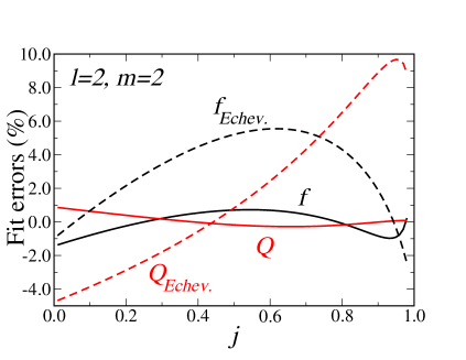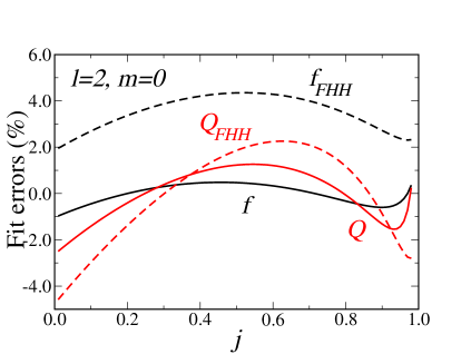The first few quasi-normal frequencies for extremal black holes asymptote to $m/2$ for $m>0$, but imposing this behavior (for instance by assuming fitting functions of the form ${\cal F}\sim m/2+f_{2}(1-j)^{f_{3}}$) usually decreases the accuracy of the fits. Indeed our fit for $l=2\,,\,m=2$ performs better than Echeverria’s, and the one for $l=2\,,\,m=0$ performs better than the fit provided in fhh . This is shown in Fig. 21, where we plot the percentage error for each of the fits, in the range $0<j<0.99$.

For the $l=|m|$ modes we can also make contact with an approach initiated by Press press and Goebel goebel , and investigated in depth by Mashhoon mashhoon , in which QNMs are regarded as waves orbiting around the unstable photon orbit, and slowly leaking out. Mashhoon’s analytical formulas were recently compared to numerical results bkkn and found to be in good agreement for $l=|m|$. This approach basically predicts that ${\cal F}_{l\pm l0}=|m|M\omega_{0}$, where $\omega_{0}$ is the co-rotating (counter-rotating) orbital frequency at the photon orbit for positive (negative) $m$ (see bkkn for further details). The counter-rotating frequency is well approximated by $M\omega_{o}\sim-1/7+5(j-1)/147$. This implies that the fundamental $l=2,m=-2$ QNM frequency should be ${\cal F}_{2-20}=2/7+10(1-j)/147\,\simeq 0.286+0.068(1-j)$. To compare with this formula, we can do a slightly different fit to the data for $m=-2$. If we fit the data to ${\cal F}_{2-20}=b+c(1-j)$ we get $b=0.287\,,\,c=0.0805$ with a maximum error of $1.6\%$. This is in reasonable agreement with Mashhoon’s prediction. For $l=3\,,\,m=-3$ the same fit yields ${\cal F}_{3-30}=0.456+0.134(1-j)$ with $1.6\%$ maximum error, whereas Mashhoon’s prediction is ${\cal F}_{3-30}=0.428+0.102(1-j)$. Thus for negative $m\,,\,l=|m|$ we can approximate the frequencies by ${\cal F}_{l-l0}\sim|m|\left[1/7+5(1-j)/147\right]$. For positive $m$ we don’t get such good agreement with a linear fit, because $M\omega$ is a rapidly varying function of $j$. Nevertheless, for moderate to large $j$ and $l=m$ we get, using Mashhoon’s formula, ${\cal F}_{ll0}\sim|l|\left(1/2-\sqrt{3(1-j)/8}\right)$. This is in very good agreement with the numerical data.

References

- (1) E. Berti, A. Buonanno and C. M. Will, Phys. Rev. D 71, 084025 (2005).
- (2) L. Barack and C. Cutler, Phys. Rev. D 69, 082005 (2004). See also L. Barack and C. Cutler, gr-qc/0310125 v3, where an erroneous factor of 3/4 in the instrumental noise is corrected.
- (3) O. Dreyer, B. Kelly, B. Krishnan, L. S. Finn, D. Garrison and R. Lopez-Aleman, Class. Quantum Grav. 21, 787 (2004).
- (4) É. É. Flanagan and S. A. Hughes, Phys. Rev. D 57, 4535 (1998).
- (5) F. Echeverria, Phys. Rev. D 40, 3194 (1989).
- (6) L. S. Finn, Phys. Rev. D 46, 5236 (1992).
- (7) K. D. Kokkotas, T. A. Apostolatos and N. Andersson, Mon. Not. R. Astron. Soc. 320, 307 (2001).
- (8) J. D. E. Creighton, Phys. Rev. D 60, 022001 (1999).
- (9) H. Nakano, H. Takahashi, H. Tagoshi and M. Sasaki, Phys. Rev. D 68, 102003 (2003); H. Nakano, H. Takahashi, H. Tagoshi and M. Sasaki, Prog. Theor. Phys. 111, 781 (2004).
- (10) Y. Tsunesada, N. Kanda, H. Nakano, D. Tatsumi, M. Ando, M. Sasaki, H. Tagoshi and H. Takahashi, Phys. Rev. D 71, 103005 (2005).
- (11) H. R. Beyer, Commun. Math. Phys. 204, 397 (1999).
- (12) H. R. Beyer, Commun. Math. Phys. 221, 659 (2001).
- (13) H.-P. Nollert, R. H. Price, J. Math. Phys. 40, 980 (1999).
- (14) H.-P. Nollert, Characteristic Oscillations of Black Holes and Neutron Stars: From Mathematical Background to Astrophysical Applications, unpublished Habilitationsschrift (2000).
- (15) N. Szpak, unpublished (gr-qc/0411050).
- (16) E. W. Leaver, Phys. Rev. D 34, 384 (1986); Erratum, Phys. Rev. D 38, 725 (1988).
- (17) N. Andersson, Phys. Rev. D 51, 353 (1995).
- (18) N. Andersson, Phys. Rev. D 55, 468 (1997).
- (19) K. Glampedakis, N. Andersson, Phys. Rev. D 64, 104021 (2001).
- (20) K. D. Kokkotas and B. G. Schmidt, Living Rev. Rel. 2, 2 (1999); H.-P. Nollert, Class. Quantum Grav. 16, R159 (1999).
- (21) S. A. Teukolsky, Astrophys. J. 185, 635 (1973).
- (22) E. Berti, V. Cardoso and M. Casals, Phys. Rev. D 73, 024013 (2006).
- (23) In the Schwarzschild limit, analogous expansions of the gravitational wave amplitude in terms of the Zerilli and Regge-Wheeler functions can be found in: A. Nagar and L. Rezzolla, Class. Quant. Grav. 22, R167 (2005).
- (24) W. Krivan, P. Laguna, P. Papadopoulos and N. Andersson, Phys. Rev. D 56, 3395 (1997).
- (25) N. Dorband, E. Berti, P. Diener, E. Schnetter and M. Tiglio in preparation.
- (26) K. Oohara and T. Nakamura, Prog. Theor. Phys. 70, 757–771 (1983); M. Sasaki and T. Nakamura, Prog. Theor. Phys. 67, 1788–1809 (1982); Y. Kojima and T. Nakamura, Prog. Theor. Phys. 71, 79–90 (1984).
- (27) J. Baker, M. Campanelli, C. O. Lousto and R. Takahashi, Phys. Rev. D 65, 124012 (2002).
- (28) R. A. Araya-Góchez, Mon. Not. R. Astron. Soc. 355, 336 (2004).
- (29) D. Markovic, Phys. Rev. D 48, 4738 (1993).
- (30) D. N. Spergel, et al., Astrophys. J. Suppl. 148, 175 (2003).
- (31) C. F. Gammie, S. L. Shapiro and J. C. McKinney, Astrophys. J. 602, 312 (2004).
- (32) U. Sperhake, B. Kelly, P. Laguna, K. L. Smith, E. Schnetter, Phys. Rev. D 71, 124042 (2005).
- (33) R. Narayan, New J. Phys. 7, 199 (2005).
- (34) K. J. Rhook and J. S. B. Wyithe, Mon. Not. Roy. Astron. Soc. 361, 1145 (2005).
- (35) E. Berti, V. Cardoso and C. M. Will, gr-qc/0601077.
- (36) A. Buonanno, Y. Chen and T. Damour, gr-qc/0508067.
- (37) C. L. Fryer, D. E. Holz and S. A. Hughes, Astrophys. J. 565, 430 (2002).
- (38) D. Merritt and M. Milosavljević, Living Rev. Relativ. 8, 8 (2005).
- (39) P. Anninos, D. Bernstein, S. R. Brandt, D. Hobill, E. Seidel and L. Smarr, Phys. Rev. D 50, 3801 (1994).
- (40) P. Anninos and S. Brandt, Phys. Rev. Lett. 81, 508 (1998).
- (41) G. Allen, K. Camarda and E. Seidel, gr-qc/9806036.
- (42) P. Anninos, R. H. Price, J. Pullin, E. Seidel and W. M. Suen, Phys. Rev. D 52, 4462 (1995).
- (43) A. M. Abrahams and G. B. Cook, Phys. Rev. D 50, R2364 (1994).
- (44) M. Saijo, T. W. Baumgarte, S. L. Shapiro and M. Shibata, Astrophys. J. 569, 349 (2002); M. Shibata and S. L. Shapiro, Astrophys. J. 572, L39 (2002); S. L. Shapiro and M. Shibata, Astrophys. J. 577, 904 (2002).
- (45) C. T. Cunningham, R. Price and V. Moncrief, Astrophys. J. 224, 643 (1978).
- (46) L. Baiotti, I. Hawke, L. Rezzolla and E. Schnetter, Phys. Rev. Lett. 94, 131101 (2005).
- (47) L. L. Scharf and P. H. Moose, IEEE Trans. Inf. Theory 22, No. 1, 11 (1976).
- (48) M. Shahram and P. Milanfar, IEEE Transactions on Signal Processing 53, 2579 (2005).
- (49) P. Milanfar and A. Shakouri, Proceedings of the International Conference on Image Processing, 864 (2002).
- (50) S. Finn and K. S. Thorne, Phys. Rev. D 62, 124021 (2000).
- (51) S. L. Larson, W. A. Hiscock and R. W. Hellings, Phys. Rev. D 62, 062001 (2000).
- (52) The Sensitivity Curve Generator was originally written by Shane Larson and may be found online at http://www.srl.caltech.edu/~shane/sensitivity/MakeCurve.html
- (53) G. Nelemans, L. R. Yungelson and S. F. Portegies Zwart, Astron. and Astrophys. 375, 890 (2001).
- (54) A. J. Farmer and E. S. Phinney, Mon. Not. R. Astron. Soc. 346, 1197 (2003).
- (55) Beside a factor 2 difference, the authors in smilanfar use a slightly different notation for the signal-to-noise: What they call SNR is really and is defined as . They assume white noise, which is certainly a good approximation for their sine signal, and is also a good approximation for our purposes. The noise probability distribution function is a Gaussian, and therefore the power spectral density (which we call ) is equal to , for a sampled process. Thus their definition is the same, apart from these nuances.
-
(56)
The right-tail probability (which is
usually denoted by , but we don’t want the reader to confuse this
with the factor) is defined as the probability of a random
variable exceeding a given value ,
where is the distribution function. For a Gaussian with mean and variance we have(79) (80) - (57) E. W. Leaver, Proc. R. Soc. London A402, 285 (1985).
- (58) H. E. Seidel and S. Iyer, Phys. Rev. D 41, 374 (1990).
- (59) H. Onozawa, Phys. Rev. D 55, 3593 (1997).
- (60) E. Berti and K. D. Kokkotas, Phys. Rev. D 68, 044027 (2003); E. Berti, V. Cardoso, K. D. Kokkotas and H. Onozawa, Phys. Rev. D 68, 124018 (2003); E. Berti, V. Cardoso and S. Yoshida, Phys. Rev. D 69, 124018 (2004). For a review see E. Berti, gr-qc/0411025.
- (61) W. Press, Astrophys. J. 170, L105 (1971).
- (62) C. G. Goebel, Astrophys. J. Lett. 172, L95 (1972).
- (63) B. Mashhoon, Phys. Rev. D 31, 290 (1985).
- (64) E. Berti and K. D. Kokkotas, Phys. Rev. D 71, 124008 (2005).