Recent analytical and numerical techniques applied to the Einstein equations

Abstract

Combining deeper insight of Einstein’s equations with sophisticated numerical techniques promises the ability to construct accurate numerical implementations of these equations. We illustrate this in two examples, the numerical evolution of “bubble” and single black hole spacetimes. The former is chosen to demonstrate how accurate numerical solutions can answer open questions and even reveal unexpected phenomena. The latter illustrates some of the difficulties encountered in three-dimensional black hole simulations, and presents some possible remedies.

1 Introduction

Extracting the full physical content from Einstein’s equations has proven to be a difficult task. The complexity of these equations has allowed researchers only a peek into the rich phenomenology of the theory by assuming special symmetries and reductions. Computational methods, however, are opening a new window into the theory. To realize the full utility of computational solutions in exploring Einstein’s equations, several questions must first be addressed. Namely, a deeper understanding of the system of equations and its boundary conditions, the development and use of more refined numerical techniques and an efficient use of the available computational resources.

In recent years, considerable advances have been made in some of these issues, allowing for the analysis of complex physical systems which arguably must be tackled numerically. In the present article we highlight some recent analytical and numerical techniques and apply them to two practical applications. The first application is the numerical evolution of bubble spacetimes in five-dimensional Kaluza-Klein theory. We study their dynamical behavior, the validity of cosmic censorship –in a set-up which a-priori would appear promising to give rise to violations of the conjecture– and reveal the existence of critical phenomena. As a second application, we discuss the numerical evolution of single black hole spacetimes. Here we consider some analytical and numerical difficulties in modeling these systems accurately. We discuss a method to alleviate some of these problems, and present tests to demonstrate the promise of this method.

2 Analytical and Numerical tools

In the Cauchy formulation of General Relativity, Einstein’s field equations are split into evolution and constraint equations. Numerical solutions are found by specifying data on an initial spacelike slice, subject to the constraints, and by integrating the evolution equations to obtain the future development of the data. Owing to finite computer resources, one is forced to use finite, and, in practice, rather small computational domains to discretize the problem. This raises several important issues.

The fundamental property for any useful numerical solution is that the solution must convergence to the continuum solution in the limit of infinite resolution. A prerequisite for a well-behaved numerical solution is a well-posed continuum formulation of the initial-boundary value problem. In certain cases, the well-posed continuum problem can then be used to construct stable numerical discretizations for which one can a priori guarantee convergence. In particular, this can be achieved for linear, first-order, symmetric hyperbolic systems with maximally dissipative boundary conditions gko ; strand ; olsson . This is briefly discussed in Sec. 2.1, for a detailed description and an extension to numerical relativity see Refs. paperI ; paperII ; paperIII ; Calabrese:2002ej .

The application of these ideas in general relativity is, naturally, more complicated. First, Einstein’s equations are nonlinear and so it is much harder to a priori prove convergence. However, a discretization that guarantees stability for the linearized equations should already be useful for the nonlinear equations, especially for those systems with smooth solutions as expected for the Einstein equations when written appropriately. This is because in a small enough neighborhood of any given spacelike slice, the numerical solution can be modeled as a small amplitude perturbation of the continuum solution.

The constraint equations in general relativity bring additional complications and greatly restrict the freedom in specifying boundary and initial data. This is illustrated and further discussed in Section 2.2. Section 2.3 discusses issues regarding the stability of the constraint manifold. The manifold is invariant with respect to the flow defined by the evolution system in the continuum problem. Numerically, however, small errors in the solution arising from truncation or roundoff error may lead to large constraint violations if the constraint manifold is unstable. Section 2.3 discusses a method for suppressing such rapid constraint violations.

2.1 Guidelines for a stable numerical implementation.

A simple numerical algorithm, or “recipe,” can be followed to solve first order, linear symmetric hyperbolic equations with variable coefficients and maximally dissipative boundary conditions, for which stability can be guaranteed. It is based on finite difference approximations with spatial difference operators that satisfy the summation by parts (SBP) property. This property is a discrete analogous of integration by parts, which is used in the derivation of energy estimates, a key ingredient for obtaining a well posed formulation of the continuum problem. SBP allows to obtain similar energy estimates for the discrete problem.

Employ spatial difference operators that satisfy SBP on the computational domain.

For the sake of simplicity, consider a set of linear, first order symmetric hyperbolic equations in the one-dimensional domain $x\in(a,b)$ which is discretized with points $x_{j}=a+j\Delta x$, $j=0\ldots N$, where $\Delta x=(b-a)/N$. Now let us introduce the discrete scalar product,

$$(u,v):=\Delta x\sum_{i,j=0}^{N}\sigma_{ij}u_{i}v_{j}\,,$$ (1)

for some positive definite matrix with elements $\sigma_{ij}$ which in the continuum limit $\Delta x\to 0$ approaches the $L_{2}$ norm $\langle u,v\rangle:=\int_{a}^{b}uv\,dx$. At the continuum level, the derivative operator $d/dx$ and scalar product satisfy integration by parts, i.e. $\langle du/dx,v\rangle+\langle u,dv/dx\rangle=uv|_{a}^{b}$, which in the discrete case is translated into a finite difference operator $D$ which satisfies $(Du,v)+(u,Dv)=uv|_{a}^{b}$ and approaches $d/dx$ in the continuum limit. The simplest difference operator and scalar product satisfying SBP are

$$\begin{array}[]{lll}Du=(u_{i+1}-u_{i})/\Delta x\,,&\sigma_{00}=\frac{1}{2}&\mbox{ for }i=0\\ Du=(u_{i+1}-u_{i-1})/(2\Delta x)\,,&\sigma_{ii}=1&\mbox{ for }i=1\ldots N-1\\ Du=(u_{i}-u_{i-1})/\Delta x\,,&\sigma_{NN}=\frac{1}{2}&\mbox{ for }i=N\end{array}$$ (2)

where the scalar product is diagonal: $\sigma_{ij}=0$ for $i\neq j$. Higher order operators satisfying SBP have been constructed by Strand strand . Additionally, when dealing with non-trivial domains containing inner boundaries, additional complexities must be addressed to attain SBP, see Ref. paperI . The finite operator $D$ is then used for the discretization of the spatial derivatives in the evolution equations, thus obtaining a semi-discrete system.

Impose boundary conditions via orthogonal projections olsson .

This ensures the consistent treatment of the boundaries, guaranteeing the correct handling of modes propagating towards, from and tangential to the boundaries. An energy estimate can be obtained for the semi-discrete system.

Implement an appropriate time integration algorithm.

The resulting semi-discrete system constitutes a large system of ODE’s which can be numerically solved by using a time integrator that satisfies an energy estimate kreiss-wu ; tadmor .

Consider adding explicit dissipation

It is well known that finite difference approximations do not adequately represent the highest frequency modes on a given grid, corresponding to the shortest possible wavelengths that can be represented on the grid. If the smallest spacing between points is $\Delta$, the shortest wavelength is $\lambda_{min}=\Delta$ with the corresponding frequency $k_{max}=2\pi/\lambda_{min}$. These modes can, and often do, travel in the wrong direction. For this reason, it is sometimes useful to add explicit numerical dissipation to rid the simulation of these modes in a way that is consistent with the continuum equation at hand. As finer grids are used, the effect of this dissipation becomes smaller and acts only on increasingly higher frequencies. The dissipation operators are constructed such that discrete energy estimates, obtained using SBP, are not spoiled. Explicit expressions for such dissipation operators are presented in Ref. paperI .

To summarize, beginning with a well-posed initial-boundary value problem, we mimic the derivation of continuum energy estimates for the discrete problem using (1) spatial derivative operators satisfying summation by parts, (2) orthogonal projections to represent boundary conditions and (3) choosing an appropriate time integrator.

2.2 Constraint-preserving boundary conditions

As discussed above, a numerical implementation of any system of partial differential equations necessarily involves boundaries. Unless periodic boundary conditions can be imposed, as is often the case for the evolution on compact domains without boundaries, one deals with an initial-boundary value problem, and thus has to face the question of how to specify boundary conditions. In theories that give rise to constraints, like general relativity, such conditions must be chosen carefully to ensure that the constraints propagate.

As a very simple illustration, consider the 1d wave equation $u_{,tt}=u_{,xx}$ on the half line $x>0$. Let us reduce it to first order form by introducing the variables $f\equiv u_{,x}$ and $g\equiv u_{,t}-bu_{,x}$, with $b$ a negative constant:

$$u_{,t} = b\,u_{,x}+g,$$ (3)

$$g_{,t} = -b\,g_{,x}+(1-b^{2})f_{,x}\;,$$ (4)

$$f_{,t} = g_{,x}+b\,f_{,x}\;.$$ (5)

At the boundary $x=0$, the system has two ingoing fields, given by $u$ and $v_{in}\equiv g+b\,f-f$, and one outgoing field. However, the ingoing fields cannot be given independently, as we see next. The constraint $C\equiv f-u_{,x}=0$ propagates as $C_{,t}=b\,C_{,x}$ and so $C$ is an ingoing field with respect to $x=0$. Therefore, we have to impose the boundary condition $C=0$ which implies the condition $u_{,x}=f$ on the main variables. We can replace this with a condition that is intrinsic to the boundary by using the evolution equation (3) in order to eliminate the $x$-derivative and obtain

$$u_{,t}=b\,f+g.$$ (6)

This equation provides an evolution equation for determining $u$ at the boundary, which guarantees that the constraint $C=0$ is preserved throughout evolution. It can be complemented by the Sommerfeld condition $v_{in}=0$.

This simple example gives just a glimpse of the different issues involved in prescribing constraint-preserving boundary conditions. The case of Einsteins’s field equations is more complicated; we refer the interested reader to Refs. CPBC-Stu ; FN ; CPBC-IR ; CPBC-SSW ; CPBC-BB ; CPBC-CLT ; CPBC-SW ; CPRST ; CS ; CPBC-Frittelli ; GMG ; LS-FatMax ; RS-FatMax . A major difficulty is the fact that, in general, constraint-preserving boundary conditions do not have the form of maximal dissipative boundary conditions, and for this reason it has proven to be difficult to find well posed initial-boundary value formulations of Einstein’s equations that preserve the constraints.

2.3 Dealing with “too many” formulations. Parameters via constraint monitoring

Formulations of the Einstein equations are often cast in symmetric hyperbolic form by adding constraints to the evolution equations multiplied by parameters or spacetime functions. The symmetric hyperbolicity condition partially restricts these parameters, however, considerable freedom in the formulation exists in choosing these free parameters (see, for instance, kst ). Analytically, when data are on the constraint surface, all allowed values for these parameters are equally valid. Off of the constraint surface, however, different values of these parameters may be regarded as representing “different” theories. It is no surprise then that numerical simulations are sensitive to the values chosen for these parameters, as numerical data rarely are on the constraint surface. Unfortunately, the parameters in current simulations are proving to be extremely sensitive. Relatively mall variations in these parameters (within the allowed range for a symmetric hyperbolic formulation) produce run times in simulations that vary over several orders of magnitude, as measured by an asymptotic observer.

Furthermore, the parameters are not unique. Values convenient for one physical problem might be inappropriate in another. Recently, a method to dynamically choose these parameters—promoted to functions of time—was introduced that naturally adapts to the physical problem under study dyn . Basically, one exploits the freedom in choosing these functions to control the growth rate of an energy norm for constraint violations. Since this norm is exactly zero analytically, this provides a guide to choosing the parameters that will drive the solution to one that satisfies the constraints. This method provides a practical solution to this problem of choosing parameters, although it may not be the most elegant solution. Ideally, one would like to understand how the growth rate of the solution depends on the these parameter values in order to choose them appropriately. This would require sharp growth estimates, however, which are still unavailable. While further understanding is gained in this front, this practical remedy can be of much help in present simulations. We summarize here the essential ideas of this method.

Consider a system of hyperbolic equations with constraint terms, $C_{c}$, written schematically as

$$\dot{u}_{a}=\sum_{b}A^{b}(u,t,\vec{x})\partial_{b}u_{a}+B_{a}(u,t,\vec{x})+\sum_{c}\mu_{ac}C_{c}(u,\partial_{j}u)\;,$$ (7)

where $u_{a}$, $B_{a}$ and $C_{c}$ are vector valued functions, and $\mu_{ac}$ is a matrix (generally not square) that is a function of the spacetime ($C_{c}$ represents a vector function of general constraint variables). The indices $\{a,b,c\}$ range over each element of the vector or matrix functions, while the indices $\{i,j,k\}$ label points on a discrete grid. We define an energy or norm of the discrete constraint variables as

$${\cal N}(t)=\frac{1}{2n_{x}n_{y}n_{z}}\sum_{c}\sum_{ijk}C_{c}(t)^{2},$$ (8)

where $n_{x}$, $n_{y}$, $n_{z}$ are the number of points in each direction. The grid indices $\{i,j,k\}$ are suppressed to simplify the notation. The time derivative of the norm can be calculated using Eq. (7)

$$\dot{\cal N}={\cal I}^{hom}+\mbox{Tr}(\mu{\cal I}^{\mu}),$$ (9)

and therefore can be known in closed form provided the matrix valued sums

$${\cal I}^{hom} = \sum_{ijk}\sum_{a,b}\frac{C_{a}}{n_{x}n_{y}n_{z}}\left[\frac{\partial C_{a}}{\partial u_{b}}+\sum_{k}\frac{\partial C_{a}}{\partial D_{k}u_{a}}D_{k}\right]\times$$ (10)

$$\left[\sum_{c}(A^{c}D_{c}u_{b})+B_{b}\right]$$

$${\cal I}^{\mu}_{bc} = \sum_{ijk}\sum_{a}\frac{C_{a}}{n_{x}n_{y}n_{z}}\times$$ (11)

$$\left[\frac{\partial C_{a}}{\partial u_{b}}+\sum_{k}\frac{\partial C_{a}}{\partial D_{k}u_{b}}D_{k}\right]C_{c}$$

are computed during evolution. Here $D_{i}$ is the discrete derivative approximation to $\partial_{i}$. We then use the dependence of the energy growth on the free constraint-functions to achieve some desired behavior for the constraints, i.e., solving Eq. (9) for $\mu_{ac}$. For example, if we choose

$$\dot{\cal N}=-a{\cal N},\qquad a>0,$$ (12)

any violation of the constraints will decay exponentially

$${\cal N}(t+\triangle t)={\cal N}(t)e^{-a\triangle t}\;.$$ (13)

As discussed in Ref. dyn , one good option among many others seems to be choosing a tolerance value, $T$, for the norm of the constraints that is close to the initial discrete value, and solving for $\mu_{ac}$ such that the constraints decay to this tolerance value after a given relaxation time. This can be done by adopting an $a$ such that after some time $\tau\equiv n_{a}\triangle t$ the constraints have the value $T$. Replacing ${\cal N}(t+\triangle t)$ by $T$ in equation (13) and solving for $a$ gives

$$a(t)=-\frac{1}{\tau}\ln{\left(\frac{T}{{\cal N}(t)}\right)}\;.$$ (14)

If one then solves

$$\dot{\cal N}=-a{\cal N}={\cal I}^{hom}+\mbox{trace}(\mu\times{\cal I}^{\mu})$$ (15)

for $\mu$, with $a$ given by Eq. (14), the value of the norm ${\cal N}(t+\tau)$ should be $T$, independent of its initial value. Therefore, Eq. (15) serves as a guide to formulate a practical method to choose free parameters in the equations with which the numerical solution behaves well with respect to the satisfaction of the constraints. Naturally, if one deals, as it is often the case, with more than one free parameter, Eq. (15) must be augmented with other conditions to yield a unique solution. This extra freedom is actually very useful in preventing large time-variations in the parameters that are sometimes needed in order to keep the constraints under control. These large variations do not represent a fundamental problem but a practical one, due to the small time stepping that they require in order to keep errors due to time integration reasonably small. One way to prevent this is by using this extra freedom to pick up the point in parameter space that not only gives the desired constraint growth, but also minimizes the change of parameters between two consecutive timesteps.

Rather than including the full details on the particular way we have implemented the method, we describe here a simple example to illustrate its application. Assume, for instance, that within a particular formulation only two free functions, $\{\kappa,\omega\}$, are employed, Eq. (15) formally evaluates to

$$\dot{\cal N}=-a{\cal N}={\cal I}^{hom}+\kappa{\cal I}^{\kappa}+\omega{\cal I}^{\omega}.$$ (16)

Now, we exploit the freedom in the free functions to adjust the rate of change of the energy ${\cal N}$ if the values of $\{{\cal I}^{hom},{\cal I}^{\kappa},{\cal I}^{\omega}\}$ are known. In practice, these are easily obtained during evolution. Once these are known, Eq. (16), coupled to the requirement that $\{\kappa,\omega\}$ vary as little as possible from one evaluation to another, results in a straightforward strategy to evaluate preferred values of the free parameters. This is done at a single resolution “test” run and, through interpolation in time, continuum, a priori defined parameters which keep the constraints under control for the given problem are obtained. Depending on the formulation of the equations, the free parameters might have to satisfy some conditions in order for symmetric hyperbolicity to hold, which can restrict the range of values these parameters can take. Nevertheless, even within a restricted window, the technique allows one to adopt the most convenient values these parameters should have for the problem at hand.

3 Applications

We now present applications of the techniques previously discussed. The goal is to illustrate how well-resolved simulations can indeed serve as a powerful tool to understand particular problems. To this end we have chosen a problem found in higher dimensional general relativity. A second application is that of the simulation of single black hole spacetimes, where the issue of the a priori lack of a preferred formulation is illustrated.

3.1 Bubble spacetimes

As a first application we concentrate on the study of bubble spacetimes and elucidate the dynamical behavior of configurations with both positive and negative masses and their possible connection to naked singularities. Bubble spacetimes have been studied extensively within five-dimensional Kaluza-Klein theory. These are five-dimensional spacetimes in which the circumference of the “extra” dimensions shrinks to zero on some compact surface referred to as the “bubble”. These bubbles were initially studied by their relevance in the quantum instability of flat spacetime witten , as bubbles can be obtained via semi-classical tunneling from it. They were later extended to include data corresponding to negative energy configurations (at a moment of time symmetry) brillpfister ; brillhorowitz . As mentioned, among the reasons for considering negative energy solutions is that naked singularities are associated with them. Therefore, these solutions are attractive tests of the cosmic censorship conjecture. Additionally, bubble spacetimes can also be obtained by double-Wick rotation of black strings, whose stability properties (or lack thereof) have been the subject of intense scrutiny in recent years. These features make bubble spacetimes both interesting an relevant for gravity beyond four-dimensions, and thus attention has been devoted to fully understand their behavior. As we will see, even when the “analytical” study of the problem is greatly simplified by symmetry assumptions, many lingering questions remain and numerical simulations provided a viable way to shed light into them. Furthermore, these simulations were also key to ‘digging out’ a few unexpected features of the solution.

In order to obtain a complete description of the dynamical behavior of these spacetimes, a numerical code, implementing Einstein equations in 5D settings, and capable of handling the possibly strong curvature associated need be constructed. Fortunately, the assumption of a ${\bf SO(3)\times U(1)}$ symmetry simplifies the treatment of the problem, which can be reduced to a $1+1$ manifold. This, in turn, renders the problem quite tractable by the currently available computational resources, though as we will see, considerable care must be placed at both analytical and numerical levels for an accurate treatment of the problem.

Initial data

We consider a generalization of the time symmetric family of initial data presented in brillhorowitz . We start with a spacetime endowed with the metric

$$ds^{2}=-dt^{2}+U(r)dz^{2}+\frac{dr^{2}}{U(r)}+r^{2}d\Omega^{2},$$ (17)

where $d\Omega^{2}=d\vartheta^{2}+\sin^{2}\vartheta d\varphi^{2}$ is the standard metric on the unit two-sphere $S^{2}$ and $U(r)$ is a smooth function that has a regular root at some $r=r_{+}>0$, is everywhere positive for $r>r_{+}$ and converges to one as $r\rightarrow\infty$. The coordinate $z$ parameterizes the extra dimension $S^{1}$ which has the period $P=4\pi/U^{\prime}(r_{+})$. The resulting spacetime $\{t,z,r\geq r_{+},\vartheta,\varphi\}$ constitutes a regular manifold with the topology $R\times R^{2}\times S^{2}$. The bubble is located where the circumference of the extra dimension shrinks to zero, that is, at $r=r_{+}$.

Additionally, we consider the presence of an electromagnetic field of the form

$$\frac{1}{2}\,F_{\mu\nu}\,dx^{\mu}\wedge dx^{\nu}=d\gamma(r)\wedge dz,$$ (18)

where $\gamma(r)$ is a smooth function of $r$ that converges to zero as $r\rightarrow\infty$. The symmetries of the problem would also allow for a non-trivial electric component of the field. However, it is not difficult to show that Maxwell’s equations imply that such a field necessarily diverges at the location of the bubble. For this reason, in the following, we only consider the case of vanishing electric field.

In this article, we consider initial data with

$$\gamma(r)=k(r_{+}^{-n}-r^{-n}),$$ (19)

where $k$ is an arbitrary constant and $n$ an integer greater than one. This field generalizes the ansatz considered in brillhorowitz , where only the case $n=2$ was discussed, and allows for different interesting initial configurations. In the time-symmetric case, initial data satisfying the Hamiltonian constraint obeys

$$U(r)=1-\frac{m}{r}+\frac{b}{r^{2}}-\frac{\tilde{k}^{2}}{r^{2n}}\,,$$ (20)

with $\tilde{k}\equiv kn/\sqrt{(n-1)(2n-1)}$ and free integration constants $m$ and $b$. Here, the parameter $m$ is related to the ADM mass via $M_{ADM}=m/4$. The fact that the bubble be located at $r=r_{+}$ requires that $0=U(r_{+})=1-\bar{m}+\bar{b}-\bar{k}^{2}$, where $\bar{m}\equiv m/r_{+}$, $\bar{b}\equiv b/r_{+}^{2}$, $\bar{k}\equiv\tilde{k}/r_{+}^{n}\,$. We also require

$$0<r_{+}U^{\prime}(r_{+})=2-\bar{m}+2(n-1)\bar{k}^{2}$$ (21)

and avoid the conical singularity at $r=r_{+}$ by fixing the period of $z$ to $P=4\pi/U^{\prime}(r_{+})$. It can be shown that the initial acceleration of the bubble area $A$ with respect to proper time is given by

$$\ddot{A}=8\pi\left[1-\bar{m}-\frac{4\bar{k}^{2}}{3}(n-1)(n-2)\right].$$ (22)

For $n=2$, as discussed in Ref. corleyjacobson , this implies that negative mass bubbles start out expanding (the initial velocity of the area is zero since we only consider time-symmetric initial data), while for large enough positive mass the bubble starts out collapsing. In the vacuum case, our numerical simulations suggest that initially collapsing bubbles undergo complete collapse and form a black string. In the non-vacuum case however, the strength of the electromagnetic field can modify this behavior completely. We will see that for small enough $k$ the bubble continues to collapse whereas when $k$ is large the bubble area bounces back and expands. Interesting behavior is obtained at the critical value for $k$ which divides the phase space between collapsing and expanding solutions.

For $n>2$ it is possible to obtain initial configurations with negative mass and negative initial acceleration SL-Rapid . This can potentially give rise to a collapsing bubble of negative energy, and thus to a naked singularity. However, our numerical results SL-Rapid suggest that cosmic censorship is valid: The bubble bounces back and starts out expanding.

Equations

In order to study the time evolution of the initial data sets given on a $t=const$ slices of the metric (17) and the electromagnetic field (18), it is convenient to introduce a new radial coordinate $R=R(r)$ which facilitates the specification of regularity conditions at the bubble location. This new coordinate is defined by

$$R(r)=\sqrt{r^{2}-r_{+}^{2}}\;,\qquad r>r_{+}\;.$$ (23)

The metric (17) now reads

$$ds^{2}=-\alpha^{2}dt^{2}+e^{2a}dR^{2}+\frac{R^{2}}{r_{+}^{2}+R^{2}}\,e^{2b}dz^{2}+(r_{+}^{2}+R^{2})e^{2c}d\Omega^{2},$$ (24)

with $\alpha=1$, $e^{-2a}=e^{2b}=(r_{+}^{2}+R^{2})U(R)/R^{2}$, $c=0$. Since $U(R)=const\cdot(R/r_{+})^{2}+O(R^{4})$ near $R=0$, and $U(R)$ converges to one in the asymptotic region, $a$ and $b$ are regular functions. An explicit example is the initial data corresponding to the zero mass Witten bubble witten where $U=1-(r_{+}/r)^{2}$ and thus $a=b=0$. When studying the time evolution of the initial data sets discussed above, we consider the metric (24) where $\alpha$, $a$, $b$ and $c$ are functions of $t$ and $R$. As we will see, the coordinate $R$ is well suited for imposing regularity conditions at the bubble location since $(R,z)$ represent polar coordinates near the bubble, $R=0$ being the center, and $z$ assuming the role of the angular coordinate. In order to avoid a conical singularity, $z$ must have the period $2\pi r_{+}e^{a-b}$. For this to be constant we need to impose the boundary condition $a(t,0)-b(t,0)=const$ at $R=0$.

Similarly, the electromagnetic field (18) is written in the form

$$\frac{1}{2}\,F_{\mu\nu}\,dx^{\mu}\wedge dx^{\nu}=\frac{R}{\sqrt{r_{+}^{2}+R^{2}}}e^{b}\left(\pi_{\gamma}dt+d_{\gamma}dR\right)\wedge dz,$$ (25)

where the functions $\pi_{\gamma}$ and $d_{\gamma}$ depend on $t$ and $R$ and satisfy $\pi_{\gamma}=0$ and $d_{\gamma}=e^{-b}\partial_{r}\gamma$ at the initial time.

We choose the following gauge condition for the lapse

$$\log(\alpha)=a+\lambda(b+2c),$$ (26)

with a parameter $\lambda$ which, in our simulations, is either zero or one. For $\lambda=1$ the resulting gauge condition is strongly related to the densitized lapse condition often encountered in hyperbolic formulations of Einstein’s equations: Indeed, the square root of the determinant of the four metric belonging to Eq. (24) is given by $\sqrt{g^{(4)}}=e^{a+b+2c}R\sqrt{r_{+}^{2}+R^{2}}\,\sin\vartheta$, so Eq. (26) sets $\alpha$ equal to the square root of the determinant of the four metric but divides the result by the factor $R\sqrt{r_{+}^{2}+R^{2}}\,\sin\vartheta$ which is singular at the bubble, at the poles $\vartheta=0,\pi/2$ and in the asymptotic region. For $\lambda=0$, the condition (26) implies that the two-metric $-\alpha^{2}dt^{2}+e^{2a}dR^{2}$ is in the conformal flat gauge. As we will see, the principal part of the evolution equations is governed by the d’Alembertian with respect to this metric. Since the two-dimensional d’Alembertian operator is conformally covariant, the resulting equations are semi-linear in that case. In particular, this implies that the characteristic speeds do not depend on the solution that is being evolved.

The field equations resulting from the five-dimensional Einstein-Maxwell equations split into a set of evolution equations and a set of constraints. The evolution equations can be written as

$$\ddot{A} = e^{-\lambda F}\left[(A^{\prime}+2G^{\prime})e^{\lambda(2B+F)}\right]^{\prime}-3(\lambda-1)(C^{\prime}+G^{\prime})^{2}e^{2\lambda B}-(\lambda+1)V$$ (27)

$$+ 2\lambda\dot{A}\dot{B}-\lambda(\lambda+1)\dot{B}^{2}-3(\lambda+1)\dot{C}^{2}+G\left[(1-\lambda)\pi_{\gamma}^{2}-(1+\lambda)e^{2\lambda B}d_{\gamma}^{2}\right],$$

$$\ddot{B} = e^{(\lambda-1)B-(\lambda+2)F}\left[B^{\prime}e^{(\lambda+1)B+(\lambda+2)F}\right]^{\prime}+\frac{3r_{+}^{2}+2R^{2}}{(r_{+}^{2}+R^{2})^{2}}\,e^{2\lambda B}$$ (28)

$$+ (\lambda-1)\dot{B}^{2}-2V,$$

$$\ddot{C} = e^{(\lambda-1)B-F}\left[(C^{\prime}+G^{\prime})e^{(\lambda+1)B+F}\right]^{\prime}-V+(\lambda-1)\dot{B}\dot{C},$$ (29)

$$+ \frac{2G}{3}\left[\pi_{\gamma}^{2}-e^{2\lambda B}d_{\gamma}^{2}\right],$$

$$\dot{\pi}_{\gamma} = e^{\lambda B-2(C+G)}\left[d_{\gamma}e^{\lambda B+2(C+G)}\right]^{\prime}+(\lambda\dot{B}-2\dot{C})\pi_{\gamma}\;,$$ (30)

$$\dot{d}_{\gamma} = \frac{\sqrt{r_{+}^{2}+R^{2}}}{R}e^{-(B-2C)}\left[\pi_{\gamma}\frac{R}{\sqrt{r_{+}^{2}+R^{2}}}e^{B-2C}\right]^{\prime}-(\dot{B}-2\dot{C})d_{\gamma}\;,$$ (31)

where we have set $A=a+\lambda b+2(\lambda+1)c$, $B=b+2c$, $C=c$ and $G=\log(r_{+}^{2}+R^{2})/2$, $F=\log(R)+G$ and $V=e^{2(A-3C)}/(r_{+}^{2}+R^{2})$. Here, and in the following, a dot and a prime denote differentiation with respect to $t$ and $R$, respectively. The evolution equations constitute a hyperbolic system on the domain $R>0$.

The constraints are the Hamiltonian and the $R$ component of the momentum constraint, given by ${\cal C}=0$, ${\cal C}_{R}=0$, where

$${\cal C} = e^{(\lambda-1)B-(\lambda+2)F}\left[e^{(\lambda+1)B+(\lambda+2)F}B^{\prime}\right]^{\prime}$$ (32)

$$+ \left[\frac{3r_{+}^{2}+2R^{2}}{(r_{+}^{2}+R^{2})^{2}}-(B^{\prime}+F^{\prime})(A^{\prime}+2G^{\prime})+3(C^{\prime}+G^{\prime})^{2}\right]e^{2\lambda B}$$

$$- V-(\dot{A}-\lambda\dot{B})\dot{B}+3\dot{C}^{2}+G\left[\pi_{\gamma}^{2}+e^{2\lambda B}d_{\gamma}^{2}\right],$$

$${\cal C}_{R} = e^{A-2C}\left[e^{-(A-2C)}\dot{B}\right]^{\prime}-(B^{\prime}+F^{\prime})\left[\dot{A}-(\lambda+1)\dot{B}\right]+2(C^{\prime}+G^{\prime})(3\dot{C}-\dot{B})$$ (33)

$$+ 2G\pi_{\gamma}d_{\gamma}\,.$$

Regularity conditions

The evolution equations contain terms proportional to $e^{-F}$ which diverge like $1/R$ near $R=0$, and therefore, regularity conditions have to be imposed at $R=0$. This is achieved by demanding the boundary conditions

$$A^{\prime}=B^{\prime}=C^{\prime}=\pi_{\gamma}=0\quad\hbox{at $R=0$}.$$ (34)

Assuming that the fields are smooth enough near $R=0$, it then follows that the right-hand side of the evolution equations is bounded for $R\rightarrow 0$. Next, as discussed above, the avoidance of a conical singularity at $R=0$ requires that $A-(\lambda+1)B=a-b$ must be constant at $R=0$. We show that this condition is a consequence of the evolution and constraint equations, and of the regularity conditions (34). Using the evolution equations in the limit $R\rightarrow 0$ and taking into account the conditions (34), we find

$$\left.\partial_{t}\left\{e^{(1-\lambda)B}\left[\dot{A}-(\lambda+1)\dot{B}\right]\right\}\right|_{R=0}=\left.-(\lambda+1)e^{(1-\lambda)B}{\cal C}\right|_{R=0}.$$ (35)

This means that if the Hamiltonian constraint is satisfied at $R=0$ (or in the case that $\lambda=-1$ even if the constraints are violated), the condition $\left.A-(\lambda+1)B\right|_{R=0}=const$ will hold provided that the initial data satisfies $\left.\dot{A}-(\lambda+1)\dot{B}\right|_{R=0}=0$. Next, we analyze the propagation of the constraint variables ${\cal C}$ and ${\cal C}_{R}$ and show that the regularity conditions (34) and the evolution equations imply that the constraints are satisfied at each time provided they are satisfied initially.

Propagation of the constraints

First, we notice that the vanishing of the momentum constraint requires that $\left.\dot{A}-(\lambda+1)\dot{B}\right|_{R=0}=0$ because of the factor $F^{\prime}$ which diverges like $1/R$ near $R=0$ in the definition of ${\cal C}_{R}$. This is precisely the condition $a(t,0)-b(t,0)=const$ discussed above. However, for this condition to hold, we first have to show that the momentum constraint actually vanishes. In order to see this, we regularize the constraint variables and define $\tilde{\cal C}=e^{F}{\cal C}$, $\tilde{\cal C}_{R}=e^{F}{\cal C}_{R}$. Now the regularity conditions (34) imply that $\tilde{\cal C}_{R}$ is regular and that $\tilde{\cal C}$ vanishes at $R=0$. As a consequence of the evolution equations and Bianchi’s identities, the constraint variables obey the following evolution system

$$\partial_{t}\tilde{\cal C} = e^{(\lambda-1)B}\partial_{R}\left[e^{(\lambda+1)B}\tilde{\cal C}_{R}\right]+(3\lambda-1)\dot{B}\tilde{\cal C},$$ (36)

$$\partial_{t}\tilde{\cal C}_{R} = e^{-(\lambda+1)B-\lambda F}\partial_{R}\left[e^{(\lambda+1)B+\lambda F}\tilde{\cal C}\right]+(\lambda-1)\dot{B}\tilde{\cal C}_{R}$$ (37)

which is regular at $R=0$. Defining the energy norm

$${\cal E}(t)=\frac{1}{2}\int_{0}^{\infty}\left(e^{2B+\lambda F}\tilde{{\cal C}}^{2}+e^{2(\lambda+1)B+\lambda F}\tilde{{\cal C}}_{R}^{2}\right)dR,$$ (38)

taking a time derivative and using the equations (36),(37) we obtain

$$\frac{d}{dt}\,{\cal E}=\left.e^{2(\lambda+1)B+\lambda F}\tilde{{\cal C}}\tilde{{\cal C}}_{R}\right|_{0}^{\infty}+\lambda\int_{0}^{\infty}\dot{B}\left(3e^{2B+\lambda F}\tilde{{\cal C}}^{2}+2e^{2(\lambda+1)B+\lambda F}\tilde{{\cal C}}_{R}^{2}\right)dR.$$ (39)

The boundary term vanishes because of the regularity conditions at $R=0$ and under the assumptions that all fields fall off sufficiently fast as $R\rightarrow\infty$. If $\dot{B}$ is smooth and bounded, we can estimate the integral on the right-hand side by a constant $C$ times ${\cal E}$, and it follows that ${\cal E}(t)\leq e^{Ct}{\cal E}(0)$. This shows that if the constraints are satisfied initially, they are also satisfied for all $t>0$ for which a smooth solution exists. In the gauge where $\lambda=0$ we even obtain the result that the norm of the constraints cannot grow in time.

To summarize, the boundary conditions (34) imply that the constraints ${\cal C}=0$, ${\cal C}_{R}=0$ and $\left.\dot{A}-(\lambda+1)\dot{B}\right|_{R=0}=0$ are preserved throughout evolution.

Outer boundary conditions

For numerical computations, our domain extends from $R=0$ to $R=R_{max}$ for some $R_{max}>0$. Now we have to replace the estimate (39) by the estimate

$$\frac{d}{dt}\,{\cal E}=\left.e^{2(\lambda+1)B+\lambda F+A_{0}}\tilde{{\cal C}}\tilde{{\cal C}}_{R}\right|_{0}^{R_{max}}+C{\cal E},$$ (40)

and it only follows that the constraints are zero if we control the boundary term at $R=R_{max}$. For this reason, we impose the momentum constraint, ${\cal C}_{R}=0$, at $R=R_{max}$. This condition results in an evolution equation for $B^{\prime}$ at the outer boundary. We combine this condition with the Sommerfeld-like conditions at $R=R_{max}$,

$$\dot{A}+A^{\prime}=0,\qquad\dot{C}+C^{\prime}=0,\qquad\pi_{\gamma}+d_{\gamma}=0.$$ (41)

Numerical implementation

Next, we discuss the numerical implementation of the above constrained evolution system. In order to apply the discretization techniques discussed in Sect. 2 we first recast the evolution equations into first order symmetric hyperbolic form by introducing the new variables $\pi_{A}=\dot{A}$, $\pi_{B}=\dot{B}$, $\pi_{C}=\dot{C}$ and $d_{A}=A^{\prime}+2G^{\prime}$, $d_{B}=B^{\prime}$, $d_{C}=C^{\prime}+G^{\prime}$. The resulting first order system is then discretized by the method of lines. Let us first discuss the spatial discretization which requires special care at $R=0$ because of the coefficients proportional to $1/R$ that appear in the evolution equations. To this end, consider the following family of toy models

$$\dot{\pi} = R^{1-n}\partial_{R}(R^{n-1}d),$$ (42)

$$\dot{d} = \partial_{R}\pi,$$ (43)

where $R>0$ is the radial coordinate, and $n=1,2,3,..$. We impose the regularity condition $d=0$ at $R=0$, which, for sufficiently smooth fields, implies that $\dot{\pi}=n\partial_{R}d$ at $R=0$, and assume that the fields vanish for $R$ sufficiently large. The toy model (42–43) corresponds to the $n$-dimensional wave equation for spherically symmetric solutions. The principal part of our evolution system has precisely this form near $R=0$, where $n$ is given by $\lambda+1$, $\lambda+3$, $2$, $1$ for the evolution equations for $\pi_{A}$, $\pi_{B}$, $\pi_{C}$ and $\pi_{\gamma}$, respectively. The system (42–43) admits the conserved energy

$$E=\frac{1}{2}\int_{0}^{\infty}R^{n-1}\left(\pi^{2}+d^{2}\right)dR.$$ (44)

A second order accurate and stable numerical discretization of the system (42–43) can be obtained as follows: We assume a uniform grid $R_{j}=j\Delta R$, $j=0,1,2...$, approximate the fields $\pi$ and $d$ by grid functions $\pi_{j}=\pi(R=R_{j})$, $d_{j}=d(R=R_{j})$, and consider the semi-discrete system

$$\dot{\pi}_{j}=R_{j}^{1-n}D_{0}(R^{n-1}d)_{j}\quad\hbox{for $j>0$ and } \dot{\pi}_{0}=\frac{n}{\Delta R}\,d_{1}\;,$$ (45)

$$\dot{d}_{j}=D_{0}\pi_{j}\quad\hbox{for $j>0$ and } \dot{d}_{0}=0\;,$$ (46)

where for a grid function $u_{j}$, $(D_{0}u)_{j}=(u_{j+1}-u_{j-1})/(2\Delta R)$ is the second order accurate centered differencing operator. It is not difficult to check that this scheme preserves the discrete energy

$$E_{discrete}=\frac{\Delta R}{2}\sum_{j=1}^{\infty}R_{j}^{n-1}\left(\pi_{j}^{2}+d_{j}^{2}\right)+\frac{\Delta R}{4n}R_{1}^{n-1}\pi_{0}^{2}$$ (47)

which proves the numerical stability of the semi-discrete system. Finally, we use a third order Runge-Kutta algorithm in order to perform the integration in time. By a theorem of Levermore tadmor , this guarantees the numerical stability of the fully discrete system for small enough Courant factor.

We apply these techniques for the discretization of our coupled system. The outer boundary conditions are implemented by a projection method. Of course, the resulting system is much more complicated than the simple toy model problem presented above, and we have no a priori proof of numerical stability. Nevertheless, we find the above analysis useful as a guide for constructing the discretization. Our resulting code is tested by running several convergence tests, and its accuracy is tested by monitoring the constraint variables ${\cal C}$ and ${\cal C}_{R}$ and the quantity $\left.\dot{A}-(\lambda+1)\dot{B}\right|_{R=0}=0$.

Results

Here we discuss the results for the numerical evolution of the initial data defined by Eqs. (17–20). We start by reviewing the evolution of the initially expanding bubbles and the initially collapsing negative mass bubbles SL-Rapid and then focus on the initially collapsing positive mass bubbles.

Brill-Horowitz initially expanding case

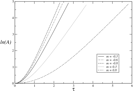
The Brill-Horowitz initial data ($n=2$) in the case of vanishing electromagnetic field is evolved. The bubble area $A$ as a function of the proper time $\tau$ at the bubble is shown in Fig. 1 for different values of the mass parameter $m$. As expected, the lower the mass of the initial configuration, the faster the expansion. Empirically, and for the parameter ranges used in our runs, we found that at late times the expansion rate obeys

$$\frac{\dot{A}}{A}\approx\frac{2-\bar{m}}{r_{+}(\tau=0)}\,,$$ (48)

where a dot denotes the derivative with respect to proper time $\tau$. In particular this approximation is valid for the bubble solution exhibited by Witten witten which describes the time evolution in the case $\bar{m}=0$.

Figure 1: Bubble area vs. proper time at the bubble. In this and the following plots, we set $r_{+}=1$. The figure shows four illustrative examples of bubbles whose initial acceleration is positive. As it is evident, the expansion of the bubble continues and the difference is the rate of the exponential expansion. The relative error in these curves, estimated from the appropriate Richardson extrapolated solution in the limit $\Delta\rightarrow 0$, is well below 0.001%.

Collapsing negative mass case

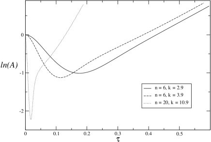
We here restrict to cases with negative masses that start out collapsing. Interestingly enough we find that even when starting with large initial negative accelerations, which in turn make the bubble shrink in size to very tiny values, it bounces back without ever collapsing into a naked singularity. As an example, Fig. 2 shows the bubble’s area versus time for different values of $n$ and $k$. The initially collapsing bubbles decrease in size in a noticeable way but this trend is halted and the bubbles bounce back and expand. Although we have not found a simple law as that in Eq. (48), clearly the bubbles expand exponentially fast. Therefore, it seems not to be possible to “destroy” the bubble and create a naked singularity. This situation is somewhat similar to the scenarios where one tries to “destroy” an extremal Reissner-Nordström black hole by attempting to drop into it a test particle with high charge to mass ratio. There, the electrostatic repulsion prevents the particle from entering the hole wald .

Figure 2: Bubble area vs. proper time at the bubble. The figure shows three illustrative examples of bubble with negative mass ($m=-0.1$ each) whose initial acceleration is negative. As it is evident, the collapse of the bubble is halted and the trend is completely reversed. The error in these curves is estimated to be well below 0.001%.

Brill-Horowitz initially collapsing case

Next, we analyze the Brill-Horowitz initial data for the case in which the bubble is initially collapsing (notice that for $n=2$ this implies that the ADM mass is positive). While our numerical simulations reveal that in the absence of the gauge field such a bubble continues to collapse, we also show that when the gauge field is strong enough, the bubble shrinks at a rate which decreases with time and then bounces back.

Obviously, if the collapse trend were not halted, a singularity should form at the origin. Since the ADM mass is positive, one expects this singularity to be hidden behind an event horizon, and one should obtain a black string. In fact, for the solutions which are initially collapsing and which have vanishing gauge field, we observe the formation of an apparent horizon. Furthermore, we compute the curvature invariant quantity $Ir_{AH}^{4}$ at the apparent horizon (as discussed in choptuikblackstring ), where $I=R_{abcd}R^{abcd}$ is the Kretschmann invariant and $r_{AH}$ the areal radius of the horizon. For a neutral black string, this invariant is $12$. Figure 3 shows how this value is attained after the apparent horizon forms for representative vacuum cases (with $m=1.1$ and $m=1.99$) this, together with the formation of apparent horizons, provides strong evidence for the formation of a black string.

Figure 3: Rescaled Kretschmann invariant $I^{0N}\equiv Ir_{AH}^{4}/12$ vs. asymptotic time for $m=1.1$ (solid line) and $1.99$ (dashed line). The first non-zero values of the lines mark the formation of the apparent horizon. After some transient period, both lines approach the value of $1$ suggesting a black string has formed.

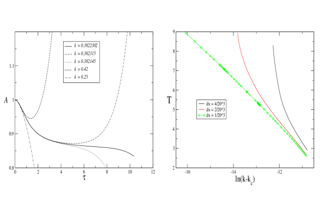
As mentioned, for strong enough gauge fields, the previously described dynamics is severely affected. Figure 4 (left panel) shows the bubble area vs. proper time for different values of $k$. For large values he bubble “bounces” back and expands while for small ones the bubble collapses. There is a natural transition region separating these two possibilities. Tuning the value of $k$ one can reveal an associated critical phenomena, the ‘critical solution’ being a member of the family of static solutions given by

$$ds^{2}=-V(r)dt^{2}+\frac{V(r)}{U(r)}dr^{2}+\frac{U(r)}{V(r)^{2}}dz^{2}+r^{2}V(r)d\Omega^{2},$$ (49)

$$\frac{1}{2}\,F_{\mu\nu}\,dx^{\mu}\wedge dx^{\nu}=\pm\frac{1}{2}\sqrt{3r_{-}(r_{+}-r_{-})}\,\frac{dr\wedge dz}{r^{2}V(r)^{2}}\,,$$ (50)

where $V(r)=1-r_{-}/r$ and $U(r)=1-r_{+}/r$. The parameters $r_{-}$ and $r_{+}$ $(>r_{-})$ are related to the period of the $z$ coordinate and to the ADM mass via $P=4\pi r_{+}(1-r_{-}/r_{+})^{3/2}$ and $M_{ADM}=r_{+}/4$. Since the quantities $P$ and $M_{ADM}$ are conserved, the member of the family of static solutions the dynamical solution approaches to can be determined a priori from the initial data.

Figure 4 (right panel) displays the time $T$ defined as the length of asymptotic time during which the bubble’s area stays within $1\%$ of the minimum value attained when the bubbles bounces back. This is a measure of how long the solution stays close to the static solution as a function of the parameter $k$. Empirically, we find the law

$$T=-r_{+}\Gamma\log|k-k_{c}|+T_{1},$$ (51)

with a parameter $\Gamma\approx 1.2$ that does not seem to depend on the family of initial data chosen. This universality property is reinforced by the linear stability analysis of the critical solutions (49,50) performed in Ref. SL-Stability where we prove that each solution has precisely one unstable linear mode growing like $\exp(\Omega t/r_{+})$ with a universal Lyapunov exponent of $\Omega\approx 0.876$. This explains the law (51) with $\Gamma=1/\Omega\approx 1.142$.

Figure 4: Left Panel. Area values vs. proper time at the bubble for different values of $k$ and $m=1.1$. By tuning the value of $k$ appropriately, the amount of time that the area remains fairly constant can be extended for as long as desired. Right Panel The time $T$ which is a measure of how long the solution stays close to the static solution vs. the logarithm of the difference between the parameter $k$ and its critical value. A linear interpolation gives the value $\gamma\approx 1.2$.

3.2 Black holes

As one of the applications that we have chosen to illustrate the use of the techniques previously discussed we consider here the evolution of single non-spinning black holes. Even when the data provided correspond to spherically symmetric and vacuum scenarios, as we will see, obtaining a long term stable implementation is not a trivial task. For additional information, and a more general treatment, we refer the reader to Ref. Tiglio:2003xm .

Formulation

We adopt the symmetric hyperbolic family of formulations introduced in sarbachtiglio . This is a first order formulation whose evolved variables are given by $\{g_{ij},K_{ij},d_{kij},\alpha,A_{i}\}$ with $g_{ij}$ the induced metric on surfaces at $t=const$, $K_{ij}$ the extrinsic curvature, $d_{kij}$ are first derivatives of the metric, $d_{kij}=\partial_{k}g_{ij}$, $\alpha$ is the lapse, and $A_{i}$ are normalized first derivatives of the lapse, $A_{i}=\alpha^{-1}\partial_{i}\alpha$.

The Einstein equations written in this formulation are subject to the physical constraints, the Hamiltonian and momentum constraints, as well as non-physical constraints, which arise from the variable definitions. The non-physical constraints are

$$C_{A_{i}}=A_{i}-N^{-1}\partial_{i}N=0\;\;,\;\;C_{kij}=d_{kij}-\partial_{k}g_{ij}=0\;\;,\;\;C_{lkij}=\partial_{[l}d_{k]ij}=0.$$ (52)

The constraints are added to the field equations and the spacetime constraint-functions $\{\gamma(t),\zeta(t),\eta(t),\chi(t),\xi(t)\}$ are introduced as multiplicative factors to the constraints. While these quantities are sometimes introduced as parameters, we extend them to time-dependent functions. For simplicity in this work, we set $\zeta=-1$. Requiring that the evolution system is symmetric hyperbolic imposes algebraic conditions on these factors, and they are not all independent. If we require that all the characteristic speeds are “physical” (i.e. either normal to the spatial hypersurfaces or along the light cone), then we obtain two symmetric hyperbolic families. One family has a single free parameter, $\chi(t)$,

$$\mbox{Single constraint-function system}\left\{\begin{array}[]{ccc}\gamma&=&-\frac{1}{2}\\ \zeta&=&-1\\ \eta&=&2\\ \xi&=&-\frac{\chi}{2}\\ \chi&\neq&0\end{array}\right.$$ (53)

and another symmetric system with two varying constraint-functions $\{\eta(t),\gamma(t)\neq-1/2\}$:

$$\mbox{Two constraint-function system}\left\{\begin{array}[]{ccc}\zeta&=&-1\\ \chi&=&-\frac{\gamma(2-\eta)}{1+2\gamma}\\ \xi&=&-\frac{\chi}{2}+\eta-2\\ \gamma&\neq&-\frac{1}{2}\\ \eta&&\end{array}\right.$$ (54)

Initial data and boundaries

Initial data for a Schwarzschild black hole are given in In-going Eddington–Finkelstein coordinates. The shift $\beta^{i}$ will be considered an a priori given vector field while the lapse is evolved to correspond to the time harmonic gauge with a given source function. This gauge source function is taken from the exact solution, such that in the high-resolution limit $\alpha=(1+2M/r)^{-1/2}$.

Black hole excision is usually based on the assumption that an inner boundary (IB) can be placed on the domain such that information from this boundary does not enter the computational domain. This requirement places strenuous demands on cubical excision for a Schwarzschild black hole in Kerr-Schild, Painlevee-Gullstrand or the Martel-Poisson martelpoisson coordinates: the cube must be inside $0.37M$ in each direction. This forces one to excise very close to the singularity, where gradients in the solution can become very large, requiring very high resolution near the excision boundary to adequately resolve the solution. This requirement follows directly from the physical properties of the Schwarzschild solution in these coordinates, and is independent of the particular formulation of the Einstein equations paperIII .

With our current uniform Cartesian code, however, we do not have enough resolution to adequately resolve the Schwarzschild solution near the singularity. Thus, we place the inner boundary inside the event horizon, but outside the region where all characteristics are out-going. The difference stencils are one-sided at the inner boundary, and no boundary conditions are explicitly applied. Testing various locations we find that placing the inner boundary at $1.1M$ gives reasonable results for the resolutions we are able to use, $\triangle x=\triangle y=\triangle z=M/5,\,M/10,\,M/20$. We are working to resolve this inconsistency in our code by using coordinate systems that conform to the horizon’s geometry.

We performed numerical experiments with the outer boundary at three different locations, $5M$, $10M$ and $15M$. Boundary conditions for the outer boundary are applied using the orthogonal projection technique referenced above, by “freezing” the incoming characteristic modes. That is, their time derivative is set to zero through an orthogonal projection. This makes use of the fact that one knows that the continuum, exact solution is actually stationary. While this would not be useful in the general case, as we shall see, even in such a simplified case the constraint manifold seems to be unstable. We are currently working on extending the boundary treatment to allow for constraint-preserving boundary conditions and studying the well posedness of the associated initial-boundary value problem.

Having set up consistent initial and boundary data, in a second order accurate implementation using the techniques mentioned in section II, we now concentrate on simulating a stationary black hole spacetime. As we will see below, even in this simple system, one encounters difficulties to evolve the system for long times. In particular, as has been illustrated in several occasions, the length of time during which a reliable numerical solution is obtained varies considerably depending on the values of the free parameters in the formulation. These parameters play no role at the constraint surface; however, off this constraint surface, these parameters have a sensible impact. Hence, at the numerical level –where generic data is only approximately at this surface–, it is necessary to adopt preferred values of these parameters. These, in turn, will depend not only on the physical situation under study but also in the details of the particular implementation (order of convergence, etc). As we argued in Section II, the constraint minimization method provides a practical way to adopt these parameters. We next illustrate this in numerical simulations of Schwarzschild spacetime.

Testing constraint minimization

We concentrate here on black hole simulations performed using the symmetric hyperbolic formulation with two constraint functions. The single function family and its disadvantages for constraint minimization are discussed in Ref. Tiglio:2003xm .

Black hole numerical results

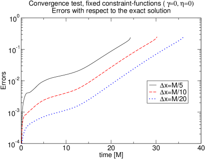
As a first attempt to numerically integrate the Einstein equations, one could simply fix the parameters $\eta$ and $\gamma$ to constant values. Lacking knowledge of preferred values for these parameters we might simply set $\eta=0$ and $\gamma=0$. Evolutions of the Schwarzschild spacetime for these parameter choices, however, show that the solution is quickly corrupted, and the solution diverges. Figure 5 shows the error in the numerical solution with respect to the exact solution for three resolutions. While the code converges, the error at a single resolution grows without bound as a function of time.

Figure 5: Two-constraint-function family, with fixed values $\gamma=0=\eta$, inner and outer boundaries at $1.1M$ and $5M$, respectively.

We now apply the constraint minimization technique to evolutions of a Schwarzschild black hole. The constraint functions $\eta(t)$ and $\gamma(t)$ will now vary in time, and both will be used to control the constraint growth. With two functions we can attempt to minimize changes in the functions themselves. This is advantageous because smoothly varying functions seem to yield better numerical results. Thus, $\eta(t)$ and $\gamma(t)$ are chosen at time step $n+1$ to minimize the quantity

$$\triangle:=\left[\eta(n+1)-\eta(n)\right]^{2}+\left[\gamma(n+1)-\gamma(n)\right]^{2}$$ (55)

$\dot{\cal N}$ is nonlinear in $\gamma$ but linear in $\eta$, allowing one to solve for $\eta$ such that $\dot{\cal N}=-a{\cal N}$,

$$\eta=\frac{-(a{\cal N}+{\cal I}^{hom}+{\cal I}^{\gamma}\gamma)(1+2\gamma)+2\gamma{\cal I}^{\chi}}{{\cal I}^{\eta}(1+2\gamma)+\gamma{\cal I}^{\chi}}$$ (56)

where, as in Section III, $a$ is given by Eq. (14). $\gamma$ is chosen from some arbitrary, large interval. The corresponding $\eta$ given by Eq. (56) is computed, and the pair $(\eta,\gamma)$ that minimizes $\triangle$ defined in Eq. (55) is chosen. $\gamma$ and $\eta$ may be freely chosen, except that $\gamma\neq-1/2$, giving two “branches”: $\gamma$ always larger than -1/2, and $\gamma$ always smaller than -1/2. We have only explored the $\gamma<-1/2$ branch using the seed values $\eta=0$, $\gamma=-1$. In order to keep the variation of the parameters between two consecutive timesteps reasonably small, we have needed to set the tolerance value for the constraints energy roughly one order of magnitude larger than the initial discretization error, and $n_{a}$ to either $10^{2}$ or $10^{3}$. This means that the constraints’ energy, though in a longer timescale, will still grow.

Figure 6: This figure shows the constraint energy and the error with respect to the exact solution. Dynamic minimization is done with boundaries at $5M$, $\triangle x=M/5$, $T=10^{-3}$, and $n_{a}=10^{3}$.

Figure 7: This figure shows the constraint functions for the run described in Figure 6.

Figure 8: Same as previous Figure, but keeping the constraint-functions constant after $750M$. The figure compares the resulting energy for the constraints with that of the previous figure (shown at late times only, since because of the setup the runs are identical up to $t=750M$).

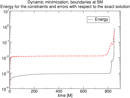
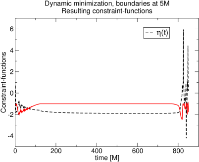
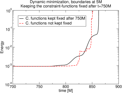
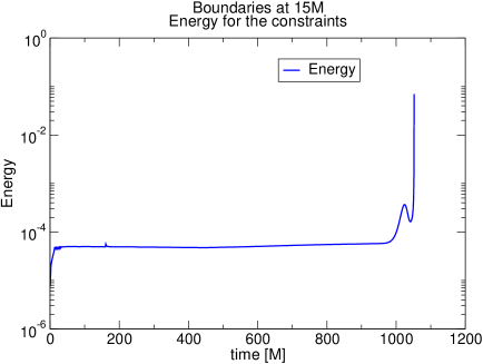
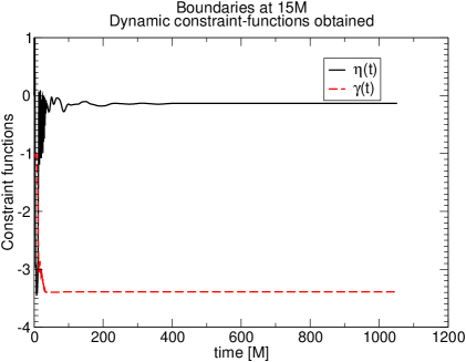
The outer boundary is first placed at $5M$. Figure 6 shows the energy of the constraints and the error with respect to the exact solution. The corresponding constraint functions are shown in Figure 7. The large variation in the functions near the end of the run appears to be a consequence of other growing errors. In Figure 8 the minimization is stopped at $750M$, and the functions are fixed to $\eta=-1.88$, $\gamma=-1.00$ for the remainder of the run. The solution diverges at approximately the same time.

Figure 9: This figure shows the black hole mass calculated from the apparent horizon with dynamic constraint-function values. The higher resolution simulation ran out of computing time. The apparent horizons were found using Thornburg’s apparent horizon finder thornburg .

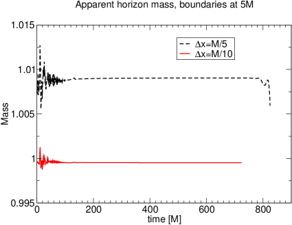
Another measure of the error in the solution is the mass of the apparent horizon, as shown in Figure 9. After some time, the mass approximately settles down to a value that is around $1.009M$, which corresponds to an error of the order of one part in one thousand. For the higher resolution, the apparent horizon mass at late times becomes indistinguishable from $1M$, given the expected level of discretization errors.

The outer boundary is now placed at $15M$. Figure 10 shows results for data equivalent to those discussed for Figure 6. The initial discretization value for the energy is $7.6459\times 10^{-6}$, and $T=10^{-5}$, $n_{a}=100$ was used. The minimization of the constraint-functions is stopped at $450M$, at which point the constraint-functions are approximately constant, and equal to

$$\eta=-1.35\times 10^{-1}\;\;\;,\;\;\;\gamma=-3.39.$$ (57)

Figure 10 shows that the dependence of the lifetime on the location of the outer boundaries is not monotonic, as for this case the code runs for, roughly, $1000M$, while with boundaries at $10M$ and $5M$ it ran for around $700M$, and $800M$, respectively. A detailed analysis of such dependence would be computationally expensive and beyond the scope of this work, and may even depend on the details of the constraint minimization, such as the values for $T$ and $n_{a}$. However, comparing Figure 5 with Figures 6–9, we see that the constraint minimization considerably improves the lifetime of the simulation, as expected.

Figure 10: Dynamic minimization done with boundaries at $15M$, $\triangle x=M/5$, $T=10^{-5}$, and $n_{a}=10^{2}$. The constraint-functions are constant for $t\geq 450M$, where they are $\eta=-0.135,\gamma=-3.389$. Thus, the constraint functions do not respond when the code is about to crash.

4 Final Words

We have chosen two problems to illustrate both the power of numerical simulations of Einstein’s equations and some of the difficulties encountered in obtaining accurate numerical solutions. This is especially relevant for black hole systems, where different poorly understood issues coupled to lack of sufficient computational power makes it much more difficult to advance at a sustained pace towards the final goal of producing a reliable description of a binary black hole system. However, it is clear that goal outweighs these difficulties. As the bubble problem illustrates, a robust implementation was not only key to responding to open questions but also proved to be the way to observing other phenomena not previously considered. Not only did it show that a priori possible way to violate cosmic censorship is invalid, but it also revealed the existence of critical phenomena, which, in turn, can be used to shed further light in the stability of black string systems SL-Stability .

Fortunately, a substantial body of work in recent years has begun to address a number of these questions. A better understanding of the initial boundary-value problem in general relativity, advances in the definition of initial data and gauge choices coupled to several modern numerical techniques are having a direct impact in current numerical efforts. It seems reasonable to speculate that if this trend continues, the ultimate goal will be within reach in a not-too-distant future.