Estimating spinning binary parameters
and testing alternative theories of gravity with LISA

Abstract

We investigate the effect of spin-orbit and spin-spin couplings on the estimation of parameters for inspiralling compact binaries of massive black holes, and for neutron stars inspiralling into intermediate-mass black holes, using hypothetical data from the proposed Laser Interferometer Space Antenna (LISA). We work both in Einstein’s theory and in alternative theories of gravity of the scalar-tensor and massive-graviton types. We restrict the analysis to non-precessing spinning binaries, i.e. to cases where the spins are aligned normal to the orbital plane. We find that the accuracy with which intrinsic binary parameters such as chirp mass and reduced mass can be estimated within general relativity is degraded by between one and two orders of magnitude. We find that the bound on the coupling parameter $\omega_{\rm BD}$ of scalar-tensor gravity is significantly reduced by the presence of spin couplings, while the reduction in the graviton-mass bound is milder. Using fast Monte-Carlo simulations of $10^{4}$ binaries, we show that inclusion of spin terms in massive black-hole binaries has little effect on the angular resolution or on distance determination accuracy. For stellar mass inspirals into intermediate-mass black holes, the angular resolution and the distance are determined only poorly, in all cases considered. We also show that, if LISA’s low-frequency noise sensitivity can be extrapolated from $10^{-4}$ Hz to as low as $10^{-5}$ Hz, the accuracy of determining both extrinsic parameters (distance, sky location) and intrinsic parameters (chirp mass, reduced mass) of massive binaries may be greatly improved.

I Introduction

The Laser Interferometer Space Antenna (LISA) is being designed to detect gravitational-wave (GW) signals in the frequency band between $10^{-4}$ Hz and $10^{-1}$ Hz danzmann . Ground-based interferometers such as LIGO, GEO, VIRGO and TAMA are sensitive in a higher frequency band, between $10$ Hz and $10^{3}$ Hz. Operating at these low frequencies, LISA can detect, among other sources, inspirals and mergers of massive black holes (MBH) with masses in the range $10^{4}\mbox{-}10^{7}M_{\odot}$. Another promising source is the inspiral and capture of stellar-mass compact objects – such as neutron stars (NS) or black holes (BH) – by intermediate-mass black holes with masses in the range $10^{2}\mbox{-}10^{5}M_{\odot}$.

Gravitational radiation reaction drives the inspiral of these binaries. The amplitude and phase of the gravitational-wave signal carry information about binary parameters, such as masses and spins, and about the location and distance of the binary. They may also be different in different theories of gravity. Therefore LISA can provide important astrophysical information, yield interesting tests of fundamental physics, and place bounds on alternative theories of gravity. In this paper, we consider, along with standard general relativity, theories of the scalar-tensor type (the simplest exemplar being that of Brans and Dicke) and theories with an effective mass in the propagation of gravitational waves (which we call massive graviton theories, for short). In scalar-tensor theories the phasing evolution is modified predominantly by the presence of dipole gravitational radiation reaction in the orbital evolution (in general relativity the lowest radiative multipole moment is the quadrupole). In massive graviton theories the gravitational wave propagation speed depends on wavelength: this generates a distortion in the time of arrival (and in the wave phasing) with respect to general relativity, similar to the dispersion of radio waves by interstellar plasma.

Previous papers willST ; willgraviton ; scharrewill ; willyunes ; damourfarese derived bounds on the graviton mass, on the Brans-Dicke parameter $\omega_{\rm BD}$ and on parameters describing more general scalar-tensor theories under the assumption that the compact objects do not carry spin. In this paper we investigate the effect of spin-orbit and spin-spin couplings both on the estimation of astrophysical parameters within general relativity, and on bounds that can be placed on alternative theories. We restrict our analysis to non-precessing spinning binaries, i.e. binaries whose spins are perpendicular to the orbital plane. The effect of non-aligned spins and the resulting precessions will be considered in future work.

Within Einstein’s general relativity, various authors have investigated the accuracy with which LISA can determine binary parameters including spin effects. Cutler CC determined LISA’s angular resolution and evaluated the errors on the binary masses and distance considering spins aligned or anti-aligned with the (orbital) angular momentum. Hughes SH investigated the accuracy with which the redshift can be estimated (if the cosmological parameters are derived independently), and considered the black-hole ring-down phase in addition to the inspiralling signal. Seto seto included the effect of finite armlength (going beyond the long wavelength approximation) and found that the distance and angular resolution accuracy improve. This happens because the response of the instrument when the armlength is finite depends strongly on the location of the source, which is tightly correlated with the distance and the direction of the orbital angular momentum. Vecchio vecchio provided the first estimate of parameters for precessing binaries when only one of the two supermassive black holes carries spin. He showed that modulational effects decorrelate the binary parameters to some extent, resulting in a better estimation of the parameters compared to the case when spins are aligned or antialigned with angular momentum. More recently, Hughes and Menou HM studied a class of binaries, which they denoted golden binaries, for which the inspiral and ring-down phases could be observed with good enough precision to carry out valuable tests of strong-field gravity.

These earlier works (except for HM ) adopted analytical approximations to LISA’s instrumental noise CC , augmented by an estimate of white-dwarf confusion noise BH in the low-frequency band. In this paper we model the LISA noise curve by a similar – albeit slightly updated – analytical approximation BC . This noise curve has the advantage of being given in analytical form, and reproduces very well the salient features of numerical noise curves available online from the LISA Sensitivity Curve Generator (SCG) SCG , a tool sponsored by the LISA International Science Team.

Our central conclusions are as follows. Inclusion of non-precessing spin-orbit and spin-spin terms in the gravitational-wave phasing generally reduces the accuracy with which the parameters of the binary can be estimated. This is not surprising, since the parameters are highly correlated, and adding parameters effectively dilutes the available information. Such an effect has already been described within Einstein’s general relativity in the context of ground-based detectors of the LIGO/VIRGO type poissonwill ; KKS . For example, for massive black-hole binaries at 3 Gpc, we find that including spin-orbit terms degrades the accuracy in measuring chirp mass by factors of order 10, and in measuring the reduced mass parameter by factors of order 20 – 100; while including spin-spin terms further degrades these accuracies by factors of order 3 and 5, respectively. For neutron stars inpiralling into intermediate-mass black holes (IMBH) with masses between 1000 and $10^{4}$ solar masses, the corresponding reductions are factors of order 20 and 5 – 30 in chirp mass and reduced mass parameter, respectively, when spin-orbit is included, and additional factors of order 4 and 7, respectively, when spin-spin terms are included.

When we consider placing bounds on alternative theories of gravity, for technical reasons, we treat only spin-orbit terms. The source of choice to place bounds on the coupling parameter $\omega_{\rm BD}$ of scalar-tensor gravity is the inspiral of a neutron star into an intermediate-mass black hole. We first reproduce results of earlier work willyunes , apart from small differences arising from corrected normalization of the LISA noise curve. Including spin-orbit effects reduces the bound on $\omega_{\rm BD}$ significantly, by factors of order 10 – 20. For example for a $1.4\,M_{\odot}$ neutron star inspiralling into a $400\,M_{\odot}$ black hole, the bound on $\omega_{\rm BD}$ goes from $8\times 10^{5}$ to $40,000$ when spin-orbit terms are included. The latter bound should be compared with the bound of $40,000$ from Cassini measurements of the Shapiro time delay bertotti .

The effect of including spin on bounding the graviton mass is more modest. In this case, the source of choice is the inspiral of binaries of massive black holes. For masses ranging from $10^{5}M_{\odot}$ to $10^{7}M_{\odot}$, the reduction in the bound induced by the inclusion of spin-orbit terms is only a factor of 4 to 5.

We consider the effect of spin terms on the angular and distance resolution of LISA. We find that spin couplings have a mild effect on the angular resolution, on the distance and, as a consequence, on the redshift determination for massive black-hole binaries. By contrast, for stellar mass objects inspiralling into intermediate-mass black holes, neither distance nor location on the sky is very well determined.

LISA can observe massive black-hole binaries with large SNR out to large values of the cosmological redshift. If the corresponding mass and distance determinations are accurate enough, LISA will be an invaluable tool to study structure formation in the early Universe. Using Monte Carlo simulations we find that LISA can provide accurate distance determinations out to redshift $z\sim 2$ for source masses $\sim 10^{7}M_{\odot}$, and out to $z\sim 4$ for source masses $\sim 10^{6}M_{\odot}$. Mass determinations strongly depend on an accurate treatment of spin effects.

Finally, we study the effect of LISA’s low-frequency sensitivity on the accuracy of estimating parameters for massive black-hole binaries (similar investigations can be found in HH and Baker ). Below $10^{-4}$ Hz, the noise characteristics of LISA are uncertain. We show, however, that if LISA’s noise spectral density can be uniformly extrapolated from $10^{-4}$ to $10^{-5}$ Hz, then the accuracy of estimating both extrinsic parameters such as distance and sky position and intrinsic parameters such as chirp mass and reduced mass, as well as the graviton mass, can be significantly higher, especially for higher-mass systems.

The paper is organized as follows. In Sec. II.1 we discuss the procedure for estimating binary parameters and the parameters of alternative theories when we average over all sky directions and binary orientations; this essentially ignores modulational effects due to the motion of the spacecraft. In Sec. II.2 we relax this assumption, and present the relevant equations for estimation for a given source direction and orientation. In Sec. II.3, we discuss the LISA noise curve to be used. Section III presents our results. In Sec. III.1 we show the results for estimates assuming averaging over directions. In Sec. III.2 we carry out a Monte Carlo analysis of $10^{4}$ binaries distributed over the angles describing the relative orientation of the binary with respect to LISA and discuss the accuracy with which binary parameters can be estimated. Though somewhat more accurate, this procedure is still affected by various approximations. In Sec. III.3 we use Monte Carlo simulations to investigate the dependence of parameter estimation on the redshift of the source. In Sec. III.4 we study the effect of the LISA low-frequency noise. Section IV summarizes our main conclusions. In Appendix A we summarize for completeness the main equations used in this paper to describe LISA’s configuration, orientation and response, as derived in Ref. CC . In Appendix B we discuss some subtleties in estimating binary parameters within the Fisher matrix formalism in alternative theories of gravity when we include spin effects.

Throughout this paper we use units in which $G=c=1$.

II Estimation of parameters in non-precessing spinning compact binaries

We assume that two independent Michelson outputs $h_{\alpha}(t)$ with $\alpha={\rm I,II}$ can be constructed from the readouts of the three LISA arms if the noise is totally symmetric (see, for example, CC ). We take two approaches to estimating parameters. In the first approach (Sec. II.1), we assume that the orientation and location of the source and the orientation of LISA are unimportant in estimating intrinsic parameters such as masses or theory-dependent parameters. These orientation dependences are contained in a number of angle-dependent functions, called pattern functions. Accordingly, we derive results using only one Michelson output, and we average over the pattern functions.

In the second approach (Sec. II.2), we are also interested in the accuracy of determination of direction and distance to the source, and thus we do not wish to average a priori over pattern functions. Instead, we carry out Monte Carlo simulations of measurements using a population of sources across the sky, and we study the distribution of accuracies of parameter estimation. In this case, we use both one and two Michelson detectors. We use the by now standard machinery of parameter estimation in matched filtering for gravitational wave detection that has been developed by a number of authors finn ; FinnChernoff ; CutlerFlanagan ; poissonwill .

II.1 Parameter estimation using pattern-function averaging

The Fourier transform of the waveform for one Michelson LISA detector, in the stationary phase approximation (SPA), and after averaging over the pattern functions, is given by

$$\tilde{h}_{\alpha}(f) = \frac{\sqrt{3}}{2}\,{\cal A}\,f^{-7/6}\,e^{{\rm i}\psi(f)}\,,\quad\quad\alpha={\rm I,II}\,,$$ (1a)

$${\cal A} = \frac{1}{\sqrt{30}\pi^{2/3}}\frac{{\cal M}^{5/6}}{D_{\rm L}}\,,$$ (1b)

where $f$ is the frequency of the gravitational waves, ${\cal M}=\eta^{3/5}M$ is the “chirp” mass, with $M=m_{1}+m_{2}$ and $\eta=m_{1}m_{2}/M^{2}$, and $D_{\rm L}$ is the luminosity distance to the source.

We have adopted the standard “restricted post-Newtonian approximation” for the waveform, in which the amplitude is expressed to the leading order in a post-Newtonian expansion (an expansion for slow-motion, weak-field systems in powers of $v\sim(M/r)^{1/2}\sim(\pi{\cal M}f)^{1/3}$), while the phasing $\psi(f)$, to which laser interferometers are most sensitive, is expressed to the highest post-Newtonian (PN) order reasonable for the problem at hand. For binaries with spins aligned (or anti-aligned) and normal to the orbital plane, this is a valid approximation because the amplitude varies slowly (on a radiation reaction timescale) compared to the orbital period. But when the spins are not aligned, modulations of the amplitude on a precession timescale must be included. Such modulations are beyond the scope of this paper.

The phasing function $\psi(f)$ is known for point masses up to 3.5 PN order blanchet1 ; blanchet2 . But spin terms are known only up to 2PN order, so to be reasonably consistent, we will include in the phasing point-mass terms only up to this same 2PN order. The needed expression for the phasing is

$$\psi(f) = 2\pi ft_{c}-\phi_{c}+\frac{3}{128}\,(\pi{\cal M}f)^{-5/3}\,\left\{1-\frac{5{\cal S}^{2}}{84\omega_{\rm BD}}\,\eta^{2/5}\,(\pi{\cal M}f)^{-2/3}-\frac{128}{3}\frac{\pi^{2}D\,{\cal M}}{\lambda_{g}^{2}\,(1+z)}\,(\pi{\cal M}f)^{2/3}\right.$$ (2)

$$+ \left.\left(\frac{3715}{756}+\frac{55}{9}\eta\right)\,\eta^{-2/5}\,(\pi{\cal M}f)^{2/3}-16\pi\,\eta^{-3/5}\,(\pi{\cal M}f)+4\beta\,\eta^{-3/5}\,(\pi{\cal M}f)\right.$$

$$+ \left.\left(\frac{15293365}{508032}+\frac{27145}{504}\eta+\frac{3085}{72}\eta^{2}\right)\,\eta^{-4/5}\,(\pi{\cal M}f)^{4/3}-10\sigma\,\eta^{-4/5}\,(\pi{\cal M}f)^{4/3}\right\}\,.$$

The structure of the phasing function is as follows: the first two terms are related to the time $t_{c}$ and phase $\phi_{c}$ of coalescence; they are parameters that essentially establish where the waveform begins or ends. The prefactor of the expression in braces, together with the first term (“1”) inside the braces, is the standard phasing from the lowest-order quadrupole approximation of general relativity. Inside the braces is a post-Newtonian expansion in powers of $v\sim(\pi{\cal M}f)^{1/3}$. The second term is the contribution of dipole gravitational radiation in Brans-Dicke theory. Let us define the scalar charge of the $i-$th body by $\alpha_{i}=\bar{\alpha}\hat{\alpha}_{i}=\bar{\alpha}(1-2s_{i})$, where $\bar{\alpha}^{2}=1/(2\omega_{BD}+3)\sim(2\omega_{BD})^{-1}$ in the limit $\omega_{BD}\gg 1$, and $s_{i}$ is called the sensitivity of the $i-$th body (a measure of the self-gravitational binding energy per unit mass). Then the coefficient in the dipole term is ${\cal S}=(\hat{\alpha}_{1}-\hat{\alpha}_{2})/2$. The fact that it is dipole radiation means that it is proportional to $v^{-2}$ compared to the quadrupole term, but the small size of $\cal S$ and the large current solar-system bound on $\omega_{\rm BD}$ make this a small correction, nevertheless. The third term in the braces is the effect of a massive graviton, which alters the arrival time of waves of a given frequency, depending on the size of the graviton Compton wavelength $\lambda_{g}$ and on a distance quantity $D$, defined below. The remaining terms in the braces are the standard general relativistic, post-Newtonian terms, including spin effects.

The quantities $\beta$ and $\sigma$ represent spin-orbit and spin-spin contributions to the phasing, given by

$$\beta = \frac{1}{12}\sum_{i=1}^{2}\chi_{i}\left[113\frac{m_{i}^{2}}{M^{2}}+75\eta\right]\hat{\mathbf{L}}\cdot\hat{\mathbf{S}}_{i}\,,$$ (3a)

$$\sigma = \frac{\eta}{48}\chi_{1}\chi_{2}\left(-247\hat{\mathbf{S}}_{1}\cdot\hat{\mathbf{S}}_{2}+721\hat{\mathbf{L}}\cdot\hat{\mathbf{S}}_{1}\hat{\mathbf{L}}\cdot\hat{\mathbf{S}}_{2}\right)\,,$$ (3b)

where $\hat{\mathbf{S}}_{i}$ and $\hat{\mathbf{L}}$ are unit vectors in the direction of the spins and of the orbital angular momentum, respectively, and $\mathbf{S}_{i}=\chi_{i}m_{i}^{2}\hat{\mathbf{S}}_{i}$. For black holes, the dimensionless spin parameters $\chi_{i}$ must be smaller than unity, while for neutron stars, they are generally much smaller than unity. It follows that $|\beta|\lesssim 9.4$ and $|\sigma|\lesssim 2.5$.

We assume that any modifications to the post-Newtonian general relativistic terms listed in the phasing formula that might be generated in Brans-Dicke theory or in massive graviton theories will be of order $1/\omega_{\rm BD}\ll 1$ or $1/(f\lambda_{g})\ll 1$ relative to those terms, and hence we will ignore such corrections.

In this paper we denote by ${\cal M}$ and $M$ the observed chirp and total masses. They are related to masses measured in the source rest frame by

$${\cal M}=(1+z){\cal M}_{\rm source}\,,\qquad M=(1+z)M_{\rm source}\,,$$ (4)

where $z$ is the cosmological redshift.

Henceforth, to simplify the notation we define

$$\varpi\equiv\frac{1}{\omega_{\rm BD}}\,,$$ (5a)

$$\beta_{g}\equiv\frac{\pi^{2}D\,{\cal M}}{\lambda_{g}^{2}\,(1+z)}\,.$$ (5b)

To estimate the binary and gravitational theory parameters, we use the standard technique of parameter estimation in matched filtering. By maximizing the correlation between a template waveform that depends on a set of parameters $\theta^{a}$ (for example, the chirp mass $\cal M$) and a measured signal, matched filtering provides a natural way to estimate the parameters of the signal and their errors. With a given noise spectral density for the detector, $S_{n}(f)$, one defines the inner product between two signals $h_{1}(t)$ and $h_{2}(t)$ by

$$(h_{1}|h_{2})\equiv 2\int_{0}^{\infty}\frac{{\tilde{h}_{1}}^{*}\tilde{h}_{2}+{\tilde{h}_{2}}^{*}\tilde{h}_{1}}{S_{n}(f)}df\,,$$ (6)

where $\tilde{h}_{1}(f)$ and $\tilde{h}_{2}(f)$ are the Fourier transforms of the respective gravitational waveforms $h(t)$. The signal-to-noise ratio (SNR) for a given $h$ is given by

$$\rho[h]\equiv(h|h)^{1/2}\,.$$ (7)

If the waveforms may be characterized by a set of parameters $\theta^{a}$, then one defines the “Fisher matrix” $\Gamma_{ab}$ with components given by

$$\Gamma_{ab}\equiv\left(\frac{\partial h}{\partial\theta^{a}}\mid\frac{\partial h}{\partial\theta^{b}}\right)\,.$$ (8)

In the limit of large SNR, if the noise is stationary and Gaussian, the probability that the GW signal $s(t)$ is characterized by a given set of values of the source parameters $\theta^{a}$ is

$$p(\mbox{\boldmath$\theta$}|s)=p^{(0)}(\mbox{\boldmath$\theta$})\exp\left[-\frac{1}{2}\Gamma_{ab}\Delta\theta^{a}\Delta\theta^{b}\right]\,.$$ (9)

where $\Delta\theta^{a}=\theta^{a}-{\hat{\theta}}^{a}$, and $p^{(0)}(\mbox{\boldmath$\theta$})$ represents the distribution of prior information. An estimate of the rms error, $\Delta\theta^{a}$, in measuring the parameter $\theta^{a}$ can then be calculated, in the limit of large SNR, by taking the square root of the diagonal elements of the inverse of the Fisher matrix,

$$\Delta\theta^{a}=\sqrt{\Sigma^{aa}}\,,\qquad\Sigma=\Gamma^{-1}\,.$$ (10)

The correlation coefficients between two parameters $\theta^{a}$ and $\theta^{b}$ are given by

$$c_{ab}=\Sigma^{ab}/\sqrt{\Sigma^{aa}\Sigma^{bb}}\,.$$ (11)

We may wish to take into account our prior information on the maximum spin; we do this in a crude way by assuming

$$p^{(0)}(\mbox{\boldmath$\theta$})\propto\exp\left[-\frac{1}{2}(\beta/9.4)^{2}-\frac{1}{2}(\sigma/2.5)^{2}\right]\,.$$ (12)

The following derivatives of $\tilde{h}$ will be needed:

$$\frac{\partial\tilde{h}}{\partial\ln{\cal A}} = \tilde{h}\,,$$ (13a)

$$\frac{\partial\tilde{h}}{\partial t_{c}} = 2\pi{\rm i}f\,\tilde{h}\,,$$ (13b)

$$\frac{\partial\tilde{h}}{\partial\phi_{c}} = -{\rm i}\,\tilde{h}\,,$$ (13c)

$$\frac{\partial\tilde{h}}{\partial\varpi} = -\frac{5{\rm i}}{3584}{\cal S}^{2}\eta^{2/5}(\pi{\cal M}f)^{-7/3}\,\tilde{h}\,,$$ (13d)

$$\frac{\partial\tilde{h}}{\partial\beta_{g}} = -\frac{{\rm i}}{\pi{\cal M}f}\,\tilde{h}\,,$$ (13e)

$$\frac{\partial\tilde{h}}{\partial\ln{\cal M}} = -\frac{5{\rm i}}{128}\,(\pi{\cal M}f)^{-5/3}\,(K_{4}v^{-2}+1+A_{4}v^{2}+B_{4}v^{3}+C_{4}v^{4})\,\tilde{h}\,,$$ (13f)

$$\frac{\partial\tilde{h}}{\partial\ln\eta} = -\frac{{\rm i}}{96}\,(\pi{\cal M}f)^{-5/3}\,(K_{5}v^{-2}+A_{5}v^{2}+B_{5}v^{3}+C_{5}v^{4})\,\tilde{h}\,,$$ (13g)

$$\frac{\partial\tilde{h}}{\partial\beta} = -\frac{3{\rm i}}{32}\,\eta^{-3/5}\,(\pi{\cal M}f)^{-2/3}\,\tilde{h}\,,$$ (13h)

$$\frac{\partial\tilde{h}}{\partial\sigma} = -\frac{15{\rm i}}{64}\,\eta^{-4/5}\,(\pi{\cal M}f)^{-1/3}\,\tilde{h}\,,$$ (13i)

where here we denote $v=(\pi Mf)^{1/3}$ and

$$K_{4} = -\frac{{\cal S}^{2}}{12}\,\varpi\,,$$ (14a)

$$A_{4} = \frac{4}{3}\left(\frac{743}{336}+\frac{11}{4}\eta\right)-\frac{128}{5}\beta_{g}\,\eta^{2/5}\,,$$ (14b)

$$B_{4} = \frac{8}{5}(\beta-4\pi)\,,$$ (14c)

$$C_{4} = 2\left(\frac{3058673}{1016064}+\frac{5429}{1008}\eta+\frac{617}{144}\eta^{2}-\sigma\right)\,,$$ (14d)

$$K_{5} = \frac{3{\cal S}^{2}}{56}\,\varpi\,,$$ (14e)

$$A_{5} = \left(\frac{743}{168}-\frac{33}{4}\eta\right)\,,$$ (14f)

$$B_{5} = \frac{27}{5}(\beta-4\pi)\,,$$ (14g)

$$C_{5} = 18\left(\frac{3058673}{1016064}-\frac{5429}{4032}\eta-\frac{617}{96}\eta^{2}-\sigma\right)\,.$$ (14h)

For all integrals appearing in the Fisher matrix we will pick the final frequency, or the upper limit of integration to be $f_{\rm fin}={\rm min}(f_{\rm ISCO},f_{\rm end})$. Here $f_{\rm ISCO}$ is twice the conventional (Schwarzschild) frequency of the innermost stable circular orbit for a point mass, namely $f_{\rm ISCO}=(6^{3/2}\pi M)^{-1}$, and $f_{\rm end}=1~{}$Hz is a conventional upper cutoff on the LISA noise curve. The initial frequency $f_{\rm in}$ in the integrals of the Fisher matrix is determined by assuming that we observe the inspiral over a time $T_{\rm obs}$ before the ISCO, and by selecting a cutoff frequency below which the LISA  noise curve is not well characterized. Our default cutoff is $f_{\rm low}=10^{-5}$ Hz; in Sec. III.4 we analyse the effects of increasing this cutoff frequency to reflect a less optimistic understanding of LISA’s low frequency noise. The initial frequency is then given, in Hz, by the larger of these frequencies,

$$f_{\rm in}={\rm max}\biggl{\{}f_{\rm low},\,4.149\times 10^{-5}\left[\frac{{\cal M}}{10^{6}M_{\odot}}\right]^{-5/8}\left(\frac{T_{\rm obs}}{1\rm yr}\right)^{-3/8}\biggr{\}}\,.$$ (15)

The frequency at a given observation time is calculated using the quadrupole approximation for radiation damping. In our calculations we assume that $T_{\rm obs}=1$ yr.

Since we anticipate setting only lower bounds on $\omega_{BD}$ and $\lambda_{g}$, we choose the nominal values $\varpi=0$ and $\beta_{g}=0$ in Eqs. (14). For simplicity, we will also assume that we are estimating spins in the case where spins are dynamically small. This is generally the case for neutron stars (see blanchetplus4 for discussion); for black holes, it means that we are considering only slowly rotating (non extremal) black holes. Consequently we also choose the nominal values $\beta=\sigma=0$ in Eqs. (14).

For a zero–spatial-curvature Universe ($\Omega_{\kappa}=0,\Omega_{\Lambda}+\Omega_{M}=1$), the luminosity distance is given by

$$D_{L}=\frac{1+z}{H_{0}}\int_{0}^{z}\frac{dz^{\prime}}{\left[\Omega_{M}(1+z^{\prime})^{3}+\Omega_{\Lambda}\right]^{1/2}}\,.$$ (16)

The quantity $D$ appearing in Eq. (5b) is defined by ($\Omega_{\kappa}=0$)

$$D=\frac{1+z}{H_{0}}\int_{0}^{z}\frac{dz^{\prime}}{(1+z^{\prime})^{2}\left[\Omega_{M}(1+z^{\prime})^{3}+\Omega_{\Lambda}\right]^{1/2}}\,,$$ (17)

(see Eq. (2.5) of willgraviton ). For the Hubble constant we assume $H_{0}=72$ km s^-1 Mpc^-1, according to the present observational estimates cosmology .

A useful quantity to characterize the effect of the various terms (Brans-Dicke, massive graviton, spin couplings and PN corrections) on the evolution of the GW frequency is the number of GW cycles accumulated within a certain frequency band. This quantity is defined as:

$${\cal N}_{\rm GW}\equiv\int_{f_{\rm in}}^{f_{\rm fin}}\,\frac{f}{\dot{f}}\,df\,.$$ (18)

To derive the number of cycles contributed by individual terms in the phasing, we use an expression for $\dot{f}$ that includes post-Newtonian GR terms, plus the Brans-Dicke and graviton-mass contributions, given by

$$\frac{df}{dt}=\frac{96}{5\pi{\cal M}^{2}}\,(\pi{\cal M}f)^{11/3}\,\left\{1+\frac{5{\cal S}^{2}\,{\varpi}}{48}\,{\eta^{2/5}}\,(\pi{\cal M}\,f)^{-2/3}+\frac{96\beta_{g}}{5}\,(\pi{\cal M}f)^{2/3}+{\rm PN\,corrections}\right\}\,,$$ (19)

where the “PN corrections” up to 2PN order, including spin terms, can be found in blanchetplus4 . When we include the massive-graviton term, the frequency $f$ and time $t$ appearing in Eq. (19) should be considered as the arrival frequency and time, respectively (the number of gravitational-wave cycles due to the massive graviton being an effective number of cycles seen by the observer at the detector location).

Contributions of individual terms in the integral (18) are generally considered significant if they exceed one wave cycle over the observation time. For various examples of the two source targets discussed in this paper, NS inspiral into IMBH, and MBH binaries, we show the individual contributions to the number of cycles, along with the initial and final frequencies, in Tables 1 and 2, respectively.

With the restricted post-Newtonian form for $\tilde{h}$ in Eq. (1), we can express the SNR $\sqrt{\langle\rho^{2}\rangle}$ in the form

$$\sqrt{\langle\rho^{2}\rangle}=6.245\times 10^{-23}\,\left(\frac{M}{M_{\odot}}\right)^{5/6}\,\eta^{1/2}\,\left(\frac{1{\rm Gpc}}{D_{L}}\right)\,\sqrt{\int_{f_{\rm in}}^{f_{\rm end}}\frac{3}{4}\frac{f^{-7/3}}{S_{h}(f)}df}\,,$$ (20)

where angular braces mean that we are averaging over LISA pattern functions.

II.2 Parameter estimation without averaging over pattern functions

In this section we consider parameter estimation without averaging over the relative orientation of the binary with respect to LISA. We assume, as in CC , that two independent Michelson outputs can be constructed from the readouts of the three LISA arms if the noise is totally symmetric. The signal measured by LISA, $h_{\alpha}(t)$ with $\alpha={\rm I,II}$, can be written as:

$$h_{\alpha}(t)=\frac{\sqrt{3}}{2}\;\frac{2m_{1}\,m_{2}}{r(t)\,D_{\rm L}}\,\tilde{A}_{\alpha}(t)\cos\;\biggl{(}\int_{0}^{t}{f(t^{\prime})\;dt^{\prime}+\varphi_{p,\alpha}(t)+\varphi_{D}(t)\biggr{)}}\,,$$ (21)

where $r(t)$ is the relative distance between the two compact bodies, $\varphi_{p,\alpha}(t)$ is the waveform polarization phase [see Eq. (43a)] and $\varphi_{D}(t)$ the Doppler phase [see Eq. (43b)]. $\tilde{A}_{\alpha}(t)$ is defined by

$$\tilde{A}_{\alpha}(t)=\sqrt{[1+(\hat{\mathbf{L}}\cdot\mathbf{n})^{2}]^{2}\,F_{\alpha}^{+\,2}+4(\hat{\mathbf{L}}\cdot\mathbf{n})^{2}\,F_{\alpha}^{\times\,2}}\,,$$ (22)

where $\hat{\mathbf{L}}$ is the orbital angular momentum unit vector, and $\mathbf{n}$ is a unit vector in the direction of the source on the sky. The quantities $F_{\alpha}^{+,\times}$ are the pattern functions, defined by Eqs. (40) and (41). The Fourier transform of the measured signal can be evaluated in the stationary phase approximation, since $\tilde{A}_{\alpha}(t)$, $\varphi_{p,\alpha}(t)$ and $\varphi_{D}(t)$ vary on time scales on the order of 1 year (thus much larger than the binary orbital period $\sim 2/f$). The result is

$$\tilde{h}_{\alpha}(f)=\frac{\sqrt{3}}{2}{\cal A}\,f^{-7/6}\,e^{i\Psi(f)}\,\left\{\frac{5}{4}\tilde{A}_{\alpha}(t(f))\right\}e^{-{\rm i}\bigl{(}\varphi_{p,\alpha}(t(f))+\varphi_{D}(t(f))\bigr{)}}\,,$$ (23)

where to 2PN order (including also the Brans-Dicke parameter and the graviton-mass term) $t(f)$ is given by

$$t(f) = t_{c}-\frac{5}{256{\cal M}}(\pi{\cal M}f)^{-8/3}\biggl{[}1-\frac{{\cal S}^{2}\,\varpi}{12}\,\eta^{2/5}\,(\pi{\cal M}f)^{-2/3}-\frac{4\,\beta_{g}}{3}\,(\pi{\cal M}f)^{2/3}$$ (24)

$$+\frac{4}{3}\left(\frac{743}{336}+\frac{11}{4}\,\eta\right)\,\eta^{-2/5}\,(\pi{\cal M}f)^{2/3}-\frac{8}{5}(4\pi-\beta)\,\eta^{-3/5}\,(\pi{\cal M}f)$$

$$+2\left(\frac{3058673}{1016064}+\frac{5429}{1008}\,\eta+\frac{617}{144}\,\eta^{2}-\sigma\right)\,\eta^{-4/5}\,(\pi{\cal M}f)^{4/3}\biggr{]}\;.$$

In Appendix A, using equations of Ref. CC , we show how to express the angular parts of $\tilde{h}_{\alpha}(f)$ in terms of the angles $\bar{\theta}_{S}$, $\bar{\phi}_{S}$, $\bar{\theta}_{L}$, $\bar{\phi}_{L}$, which describe the source location and orbital angular momentum direction in the reference frame attached to the solar system barycenter. To evaluate the Fisher matrix we use the derivatives with respect to the parameters ${\cal M}$, $\eta$, $\beta$, $\sigma$, $\phi_{c}$, $t_{c}$, ${\rm ln}\,{\cal A}$, $\varpi$ and $\beta_{g}$, given by Eqs. (13). We also determine analytically the angular derivatives with respect to $\bar{\theta}_{S}$, $\bar{\phi}_{S}$, $\bar{\theta}_{L}$, $\bar{\phi}_{L}$ using formulas given in Appendix A. The final results are lengthy and unenlightening, so we do not write them down here. We choose to evaluate the angular derivatives analytically since this is likely to be more accurate than the numerical finite-differencing adopted in Refs. CC ; SH . As before, we choose the nominal values $\varpi=\beta_{g}=\beta=\sigma=0$.

The non-averaged SNR is ($\alpha={\rm I,II}$)

$$\rho_{\alpha}(\bar{\theta}_{S},\bar{\phi}_{S},\bar{\theta}_{L},\bar{\phi}_{L})=7.807\times 10^{-23}\,\left(\frac{M}{M_{\odot}}\right)^{5/6}\,\eta^{1/2}\,\left(\frac{1{\rm Gpc}}{D_{L}}\right)\,\sqrt{\int_{f_{\rm in}}^{f_{\rm end}}\frac{3}{4}\tilde{A}^{2}_{\alpha}(t(f);\bar{\theta}_{S},\bar{\phi}_{S},\bar{\theta}_{L},\bar{\phi}_{L})\frac{f^{-7/3}}{S_{h}(f)}df}\,.$$ (25)

For some binary-mass configurations we estimate the parameters using the two LISA  detectors. In this case the Fisher matrix is

$$\Gamma_{ab}^{\rm tot}\equiv\left(\frac{\partial h_{\rm I}}{\partial\theta^{a}}\mid\frac{\partial h_{\rm I}}{\partial\theta^{b}}\right)+\left(\frac{\partial h_{\rm II}}{\partial\theta^{a}}\mid\frac{\partial h_{\rm II}}{\partial\theta^{b}}\right)\,,$$ (26)

and the rms error, $\Delta\theta^{a}$, in measuring the parameter $\theta^{a}$ is $\Delta\theta^{a}=\sqrt{\Sigma^{aa}}$ with $\Sigma=\left[\Gamma^{\rm tot}\right]^{-1}$  . The total SNR is $\rho_{\rm tot}=\sqrt{\rho_{\rm I}^{2}+\rho_{\rm II}^{2}}$.

We expect that estimates obtained for parameters such as ${\cal M}$, ${\cal\eta}$, $\beta$, $\sigma$, $\varpi$ and $\beta_{g}$ when we do not pattern average will not differ qualitatively from those obtained using pattern averaged templates. As we will see, those parameters, which appear in the phasing of the signal, are relatively uncorrelated with the parameters appearing in the amplitude, such as $\bar{\theta}_{S}$, $\bar{\phi}_{S}$, $\bar{\theta}_{L}$, $\bar{\phi}_{L}$.

II.3 Noise curve for the LISA instrument

The non-sky-averaged noise spectral density of LISA  depends on the relative orientation between the instrument and the source, and it is very hard to implement in estimating binary parameters. Generally, the LISA  community has been using the so-called sky-averaged spectral density $S_{h}^{\rm SA}$ [see e.g., Ref. FT and the LISA Pre-Phase A Report]. The sky-averaged spectral density is computed by a combination of three factors, including: (i) the raw spectral noise density $S_{n}$, (ii) the gravitational-wave transfer (response) function $R$ and (iii) the noise transfer (response) function $R_{n}$. They combine together in LHH

$$S_{h}^{\rm SA}=\frac{S_{n}\,R_{n}}{R}\,.$$ (27)

In this paper we are also interested in determining binary parameters without averaging over the source location, so we are not allowed, in principle, to use $S_{h}^{\rm SA}$. To overcome this difficulty we evaluate an effective non-sky-averaged spectral density which gives the correct result at low frequency, but is only approximately valid in the high-frequency region. In the low frequency limit, the GW transfer function used in the LISA Sensitivity Curve Generator SCG is $R=4(\sqrt{3}/2)^{2}1/5=3/5$, where the factor $(\sqrt{3}/2)^{2}$ comes from the LISA arms being at $60^{o}$, the factor 1/5 is due to the sky-average of the pattern functions ($\langle F_{+,\times}^{2}\rangle=1/5$) and the factor 4 depends on the particular read-out variable used. Since our definition of the GW signal already includes the factor $\sqrt{3}/2$ [see Eqs. (1a) and (23)], to obtain the effective non-sky-averaged spectral density we must multiply $S_{h}^{\rm SA}$ by $(\sqrt{3}/2)^{2}/5=3/20$. The final result is:

$$S_{h}^{\rm NSA}(f)=\left[9.18\times 10^{-52}\left(\frac{f}{1~{}{\rm Hz}}\right)^{-4}+1.59\times 10^{-41}+9.18\times 10^{-38}\left(\frac{f}{1~{}{\rm Hz}}\right)^{2}\right]~{}{\rm Hz}^{-1}\,,$$ (28)

and has been obtained also in Ref. BC . We estimate white-dwarf confusion noise following BC , which uses results from conf1 ; conf2 : the galactic contribution is approximated as

$$S_{h}^{\rm gal}(f)=2.1\times 10^{-45}\left(\frac{f}{1~{}{\rm Hz}}\right)^{-7/3}~{}{\rm Hz}^{-1}\,,$$ (29)

and the contribution from extra-galactic white dwarfs as

$$S_{h}^{\rm ex-gal}(f)=4.2\times 10^{-47}\left(\frac{f}{1~{}{\rm Hz}}\right)^{-7/3}~{}{\rm Hz}^{-1}\,.$$ (30)

We compute the total (instrumental plus confusion) noise as

$$S_{h}(f)={\rm min}\left\{S_{h}^{\rm NSA}(f)/{\rm exp}\left(-\kappa T^{-1}_{\rm mission}dN/df\right),~{}S_{h}^{\rm NSA}(f)+S_{h}^{\rm gal}(f)\right\}+S_{h}^{\rm ex-gal}(f)\,.$$ (31)

Here $dN/df$ is the number density of galactic white-dwarf binaries per unit gravitational-wave frequency, for which we adopt the estimate

$$\frac{dN}{df}=2\times 10^{-3}~{}{\rm Hz}^{-1}\left(\frac{1~{}{\rm Hz}}{f}\right)^{11/3}\,;$$ (32)

$\Delta f=T^{-1}_{\rm mission}$ is the bin size of the discretely Fourier transformed data for a LISA mission lasting a time $T_{\rm mission}$; and $\kappa\simeq 4.5$ is the average number of frequency bins that are lost when each galactic binary is fitted out. The factor ${\rm exp}\left(-\kappa T^{-1}_{\rm mission}dN/df\right)$ thus represents the fraction of “uncorrupted” bins where instrumental noise still dominates. At variance with BC , in our calculations we always assume that the duration of the LISA mission $T_{\rm mission}=1$ yr, consistently with the choice we made for the observation time $T_{\rm obs}$ in Eq. (15). The analytic root noise spectral density curve (31) used in this paper is shown in Fig. 1 together with the corresponding root noise spectral density curve from the LISA Sensitivity Curve Generator SCG . The SCG curve shown is obtained using the nominal values SNR=1, arm length $=5\times 10^{9}$ m, telescope diameter $=0.3$ m, laser wavelength $=1064$ nanometers, laser power $=1.0$ Watts, optical train efficiency $=0.3$, acceleration noise $=3\times 10^{-15}\,{\rm m}\,{\rm s}^{-2}\,{\rm Hz}^{-1/2}$, and position noise budget $=2\times 10^{-11}\,{\rm m}\,{\rm Hz}^{-1/2}$, with position noise setting the floor at high frequency. The data returned by the SCG is then multiplied by $\sqrt{3/20}$ to obtain the effective non-sky averaged curve shown in Fig.  1.

III Results of parameter estimation

III.1 Estimates using pattern-averaged templates

We begin with neutron-star inspirals into intermediate mass black holes. These are the best sources for bounding scalar-tensor gravity, for the following reasons. In scalar-tensor theory, dipole gravitational radiation is controlled by the difference ${\cal S}=(\hat{\alpha}_{1}-\hat{\alpha}_{2})/2$ in the rescaled scalar charge $\hat{\alpha}_{i}$ between the two bodies. We recall that $\hat{\alpha}_{i}=(1-2s_{i})$ and

$$s_{i}=\left(\frac{\partial(\ln m_{i})}{\partial(\ln G_{\rm eff})}\right)_{N}\,,$$ (33)

where $m_{i}$ is the total mass of the body, $G_{\rm eff}$ is the effective gravitational constant at the location of the body (which is related to the value there of the Brans-Dicke scalar field) and the subscript $N$ denotes that the number of baryons is held fixed. For neutron stars, $s_{i}$ can be substantial, and thus $\hat{\alpha}_{i}$ can differ markedly from unity ($\hat{\alpha}_{i}\sim 0.6-0.8$), but because it is only weakly dependent on the NS equation of state and mass zaglauer , the difference ${\cal S}$ for NS binaries is typically ${\cal S}<0.05$, so NS-NS binaries do not provide interesting bounds on Brans-Dicke theory willST (see however damourfarese for discussion of more general scalar-tensor theories). Because of the no-hair theorem, for black holes $\hat{\alpha}_{\rm BH}\equiv 0$, so BH-BH binaries cannot be used to put bounds on the Brans-Dicke parameter via dipole radiation. Therefore, following previous papers on the subject willST ; scharrewill ; willyunes , we only consider NS-BH binaries as sources for this purpose. Furthermore, as shown earlier scharrewill ; willyunes , inspiral into lower-mass black holes gives the most promising bounds, primarily because more cycles are observed in a given period of integration in that case. The event rate of such inspirals involving intermediate-mass black holes is uncertain, but is likely to be very small miller ; willimbh ; only a lucky detection of such an inspiral will lead to a suitable test. White dwarf-BH binaries could also be used to test Brans-Dicke theory, since $\hat{\alpha}_{WD}\sim 1$ ($s_{WD}\sim 10^{-4}$), so that ${\cal S}\sim 0.5$, except that tidal effects will play a role in the late stages of the inspiral, depending on the mass of the black hole (for discussion, see scharrewill ).

For concreteness we focus on four NS-BH binaries, setting the NS mass $M_{\rm NS}=1.4M_{\odot}$ and considering black holes of mass $M_{\rm BH}=400,~{}1000,~{}5000$ and $10^{4}~{}M_{\odot}$. The borderline between massive and supermassive BHs is hazy, but we choose not to consider NSs inspiralling into “supermassive” BHs with $M=10^{5}\mbox{-}10^{8}M_{\odot}$. Even in the context of pure general relativity, our approximation that the binary orbits be circular is expected to be unreliable for these high-mass cases: for high mass ratios the binary is likely to be formed by capture of the smaller body into the larger one, and the eccentricity will not be washed out by radiation reaction. Adding eccentricity complicates the analysis to a level that is beyond the scope of this paper, and we plan to return to this problem in the future.

We first consider the inspiral of these four representative binaries within general relativity (omitting the BD term in the phase). From the initial and ending frequencies listed in Table 1 we see that these binaries sweep through the high frequency part of the LISA band, say from $\sim 10^{-2}$ Hz up to $\sim 1$ Hz. In Table 3 we list the errors and correlation coefficients that are obtained when we truncate the phasing formula at various PN orders and include spin-orbit and spin-spin effects. For consistency, at 1PN order we do not include spin effects, at 1.5PN order we include only spin-orbit effects, and at 2PN order we include both spin-orbit and spin-spin effects. All results assume $\rho=10$. In the left panel of Fig. 2 we show the corresponding luminosity distance as a function of the black hole mass $M_{\rm BH}$.

From Table 3 we see that the errors on all parameters increase considerably when spin effects are taken into account. This applies in particular to the chirp mass ${\cal M}$ and the parameter $\eta$. This spin-induced degradation in parameter estimation has long been known poissonwill : it occurs because (in the absence of precessional effects) the parameters are highly correlated, so that adding parameters effectively dilutes the available information.

For technical reasons, when we consider alternative theories of gravity we only include spin-orbit effects. If in addition we include spin-spin effects the dimensionality of the Fisher matrix increases, and the matrix inversion required to obtain the correlation matrix appears to be unreliable. This issue is addressed in Appendix B.

In Table 4 we show errors and correlation coefficients for NS-BH binaries at 2PN order when we include the BD term. For nonspinning binaries the results are similar to Table I in Ref. willyunes , except that those authors used templates at 1.5PN order and did not take into account the factor $\sqrt{3}/2$ which appears in Eq. (1a). The BD term is highly correlated with ${\cal M}$ and $\eta$ ($c^{{\cal M}\varpi}$ and $c^{\eta\varpi}$ are both quite large). Correspondingly, the error on both ${\cal M}$ and $\eta$ increases by roughly one order of magnitude with respect to the “general relativistic” values listed in Table 3. We also compute the BD bound obtained by inverting only the diagonal element $\Gamma_{\varpi\varpi}$ of the Fisher matrix. This “uncorrelated” bound $\omega_{\rm BD,unc}$ is always about two orders of magnitude larger than the actual value we obtain by inverting the full Fisher matrix in the absence of spins.

Notice also that the BD bound decreases with increasing black hole mass. This can be partially understood by the following argument: the derivative of the GW signal with respect to $\varpi$ is proportional to $M^{-1}_{\rm NS}M^{-4/3}_{\rm BH}$ [see Eq. (13d) and use $M_{\rm BH}\gg M_{\rm NS}$]. Therefore the derivative decreases as $M_{\rm BH}$ increases; the integration over the frequency range (which also depends on mass) modifies this dependence somewhat, but the final conclusion is that the higher the BH mass, the lower the Brans-Dicke bound.

From Table 4 we also see that non-precessional spin effects reduce considerably the bound on the Brans-Dicke parameter. For example, for a $(1.4+1000)~{}M_{\odot}$ binary the bound decreases by a factor 10 (from $\sim 2\times 10^{5}$ to $\sim 2\times 10^{4}$) when we include the spin-orbit term. We will see later (Table 7) that a further reduction of a factor $\sim 2$ comes from inclusion of effects related to the orbital motion of LISA. We also found that including priors, that is, assuming that we know a priori from general relativity that the compact objects’ spins are bounded from above (see poissonwill for a discussion) has completely negligible effects when we include spin-orbit terms.

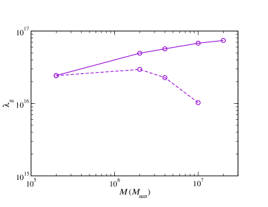
In setting bounds on the graviton mass, we consider massive and supermassive binary black holes with $M=10^{4}\mbox{-}10^{7}M_{\odot}$. The derivative of the GW signal with respect to $\beta_{g}$ is inversely proportional to the chirp mass ${\cal M}$, so for comparable-mass binaries, the higher the total mass the higher the graviton-mass bound. However, as seen from the initial and ending frequencies in Table 2, for $M_{\rm BH}>10^{7}M_{\odot}$, the binary sweeps through the low-frequency end of the LISA band below $10^{-4}$ Hz, where the predicted sensitivity of LISA  is not very robust at present. The sensitivity in this low-frequency regime depends on how efficiently the acceleration noise can be reduced. In Sec. II.2, we shall investigate the effect on the estimation of the parameters and on the graviton-mass bound, if the LISA noise curve can be trusted only down to a lower frequency $f_{\rm low}\sim 10^{-4}$ or $5\times 10^{-5}$ Hz.

In Tables 5 and 6 we list the errors and correlation coefficients when binaries with high, comparable masses are detected using pattern-averaged templates at 2PN order. Table 5 shows results for pure general relativity, with spin-orbit and spin-spin effects included. Table 6 shows results when a massive graviton term and a spin-orbit term are included. As in the BD case, we do not show results for a massive graviton combined with spin-orbit and spin-spin effects, because the inversion of the large Fisher matrix in this case appears to be unreliable (see Appendix B).

As in the case of NS-BH binaries, adding new parameters causes a degradation in the accuracy with which we can estimate parameters. All the values reported in Tables 5 and  6 are obtained for binaries at 3 Gpc. The corresponding SNR for equal mass BH-BH systems is shown in the right panel of Fig. 2 as a function of the total mass of the binary. For $M\gtrsim 10^{6}M_{\odot}$ we observe the appearance of a relative minimum, corresponding to the range of frequencies in which white-dwarf confusion noise dominates over instrumental noise.

Although we only report results for the currently favoured values of the cosmological parameters, we verified that the upper bound on the graviton wavelength depends only weakly on the underlying cosmological model. The “uncorrelated” bound $\lambda_{g,\rm unc}$ obtained by inverting only the diagonal element $\Gamma_{\beta_{g}\beta_{g}}$ of the Fisher matrix is about one order of magnitude larger than the result obtained by inverting the full Fisher matrix (for $\omega_{\rm BD}$ the difference was about two orders of magnitude). Compared with the case of scalar-tensor theories, bounds on massive graviton theories seem to be less sensitive to correlations among different parameters.

III.2 Estimates using templates without pattern averaging

To assess the effect of pattern-averaging on parameter estimation, and also to determine how accurately LISA can measure source locations and luminosity distances, we adopt the non-averaged templates of Sec. II.2, and perform Monte Carlo simulations using a population of sources across the sky. We consider in detail two systems: (i) a NS-BH binary with mass of $(1.4+1000)M_{\odot}$ observed with a single-detector SNR $\rho_{I}=10$ (a typical target system used to place bounds on the BD parameter), and (ii) a BH-BH binary with mass of $(10^{6}+10^{6})M_{\odot}$ at distance $D_{L}=3$ Gpc (a typical system in the context of massive graviton theories).

For each of these systems we distribute $10^{4}$ sources over sky position and orientation. We randomly generate the angles $\bar{\phi}_{S}$, $\bar{\phi}_{L}$ in the range $[0,2\pi]$ and $\mu_{S}=\cos\bar{\theta}_{S}$, $\mu_{L}=\cos\bar{\theta}_{L}$ in the range $[-1,1]$. As in SH , to generate random numbers we use the routine RAN2 numrec . Computing and inverting the Fisher matrix for $10^{4}$ binaries typically takes $\sim 8-15$ minutes (depending on the dimensionality of the matrix) on an ordinary laptop. This is much faster (by a factor $\sim 500$) than previous Monte Carlo simulations SHPC . A marginal difference with previous codes is that we compute angular derivatives analytically instead of using finite differencing, but the major improvement is due to our use of a numerical integrator based on spectral methods, namely the Gauss-Legendre routine GAULEG numrec . Numerical experiments show that $\sim 600$ points in the spectral expansion are sufficient to obtain an accuracy of one part in $10^{4}$ in all parameter errors. This is true even when we use splines to interpolate tabulated data from the LISA Sensitivity Curve Generator, instead of adopting the analytical noise curve of Eq. (31). When the waveform contains a large number of highly correlated parameters, computing the inverse of the Fisher matrix can be numerically difficult. The method we used to check the robustness of our results is described in Appendix B.

Once we have computed the errors for all $10^{4}$ binaries we group them into $N_{\rm bins}$ bins depending on the (logarithmic) distribution of their errors: a binary belongs to the $j$-th bin if the error on some parameter $X$ satisfies

$$\left\{\ln(X_{\rm min})+\frac{(j-1)[\ln(X_{\rm max})-\ln(X_{\rm min})]}{N_{\rm bins}}\right\}<\ln(X)\leq\left\{\ln(X_{\rm min})+\frac{j[\ln(X_{\rm max})-\ln(X_{\rm min})]}{N_{\rm bins}}\,\right\}\,,$$ (34)

for $j=1,\dots,N_{\rm bins}$. In this paper we fix $N_{\rm bins}=50$. Once we have binned the data, we normalize the binaries in each bin to the total number of binaries to get a “probability distribution” of the error on the variable $X$.

In Figs. 3 and 4 we show the resulting histograms for a NS-BH binary of $(1.4+10^{3})M_{\odot}$ with $\rho_{I}=10$. The plots contain various histograms for parameter estimations made when spins are absent, when spin-orbit is included, and when both spin-orbit and spin-spin are included. The histograms come in pairs: in each case the solid-line histogram refers to measurements carried out with only one data stream from the Michelson interferometer ${\rm I}$, the dashed histogram refers to measurements made when both data streams from Michelson interferometers ${\rm I}$ and ${\rm II}$ are combined. Not surprisingly, the accuracy is improved with the use of two outputs, very roughly by a factor of order $\sqrt{2}$ in most cases.

In Fig.  3 we plot the probability distribution for the luminosity distance $\Delta D_{L}/D_{L}$ and for the angular resolution $\Delta\Omega_{S}$, defined as

$$\Delta\Omega_{S}=2\pi|\sin\bar{\theta}_{S}|\left\{\Sigma_{\bar{\theta}_{S}\bar{\theta}_{S}}\Sigma_{\bar{\phi}_{S}\bar{\phi}_{S}}-\Sigma^{2}_{\bar{\theta}_{S}\bar{\phi}_{S}}\right\}^{1/2}\,.$$ (35)

In Fig.  4 we plot the distributions for the chirp mass $\Delta{\cal M}/{\cal M}$, the reduced mass $\Delta\mu/\mu$, the spin parameters $\Delta\beta$ and $\Delta\sigma$, and the bound on the BD parameter $\omega_{\rm BD}$. The distribution for $\Delta\mu/\mu$ can be obtained from the errors on $\eta$ and ${\cal M}$ by error propagation, taking into account that the correlation between the two mass parameters, as defined in Eq. (11), can be large:

$$\frac{\Delta\mu}{\mu}=\left[\left(\frac{\Delta{\cal M}}{{\cal M}}\right)^{2}+\left(\frac{2}{5}\frac{\Delta\eta}{\eta}\right)^{2}+\frac{4}{5}\left(\frac{\Delta{\cal M}}{{\cal M}}\right)\left(\frac{\Delta\eta}{\eta}\right)c^{{\cal M}\eta}\right]^{1/2}\,.$$ (36)

The plots contain histograms evaluated when spins are absent, when spin-orbit alone is considered and when both spin-orbit and spin-spin are included. We complement these plots by Table 7, which shows the average errors obtained summing over all binaries, both with and without the BD term. Notice that this procedure is different from averaging over the sky without taking into account the orbital motion of LISA. For each model, the first line in Table 7 refers to errors obtained averaging over all binaries and using only detector I, the second line refers to an average over all binaries using both detectors, while the third line reproduces, for comparison, the corresponding pattern-averaged results from Tables 3 and 4. In general, the pattern-averaged procedure gives good qualitative, albeit systematically low estimates of the measurement errors, compared to the Monte Carlo results. For stellar mass inspirals into intermediate-mass black holes, both the angular resolution and the distance determination accuracy are poor. The Monte Carlo simulation gives rather broad probability distributions, shown in Fig. 3, with minimum error in distance around 0.1, but with a tail extending up to $\Delta D_{L}/D_{L}\sim 10$ or so. The values for $\Delta\Omega_{S}$ in steradians look rather small, but when expressed in arcminutes, with $\delta\theta_{S}\approx[\Delta\Omega_{S}\times(3283/{\rm str})]^{1/2}\times 60$ arcmin, they are substantial. For comparison, the angular diameter of the Moon (and the Sun) as seen from the Earth is $\simeq 30$ arcmins. The angular resolution is degraded when spin terms are included, as is apparent in the top panels of Fig. 3, while the distance determination is relatively insensitive to the inclusion of spin terms. As first noticed by Cutler CC , both the angular distribution and the distance determination improve when we use both detectors (dashed lines) instead of a single detector (solid lines).

A noteworthy feature of the histograms in Fig. 4 is that the errors on ${\cal M}$, $\mu$, $\beta$, $\sigma$ and $\omega_{\rm BD}$ show a peculiar “double-peak” structure which is absent for the high-mass BH-BH binaries. We see this double-peak structure for the first time because our fast spectral integrator allows us to simulate a sufficiently high number of binaries, but we have no analytical understanding of this behavior. The inclusion of each spin-coupling term degrades the determination of both ${\cal M}$ and $\mu$ by roughly one order of magnitude. The large reduction on the Brans-Dicke bound caused by the inclusion of non-precessing spins is one of the main results of this work (bottom panel of Fig. 4).

In Figs. 5 and 6 we show similar histograms for a binary of total observed mass $(10^{6}+10^{6})M_{\odot}$ at a fixed distance of 3 Gpc, and in Table 8 we display average errors obtained by summing over all binaries. Supermassive BH-BH binaries can be observed at much higher redshifts than NS-BH binaries. LISA’s accuracy in measuring the luminosity distance $D_{L}$ can thus be exploited to infer the redshift $z$ of the source, disentangling the mass-redshift degeneracy of the waveforms and allowing the determination of the masses in the source rest frame. Indeed, Hughes proposed to use gravitational wave observations in this way to map the merger history of supermassive black holes SH . Once we have $\Delta D_{L}/D_{L}$ we can compute the error on the binary’s redshift by the following procedure. If we assume that the cosmological parameters $\Omega_{\Lambda}$ and $H_{0}$ are known with an accuracy $\simeq 10\%$, we can use error propagation to get $\Delta z$ from $\Delta D_{L}$ following Hughes SH :

$$\Delta z=\left(\frac{\partial D_{L}}{\partial z}\right)^{-1}\left[\Delta D_{L}^{2}+\left(\frac{\partial D_{L}}{\partial\Omega_{\Lambda}}\right)^{2}\Delta\Omega_{\Lambda}^{2}+\left(\frac{\partial D_{L}}{\partial H_{0}}\right)^{2}\Delta H_{0}^{2}\right]^{1/2}\,.$$ (37)

From Eq. (16), and assuming that $\Omega_{M}+\Omega_{\Lambda}=1$, we find the derivatives

$$\frac{\partial D_{L}}{\partial z} = \frac{D_{L}}{1+z}+\frac{1+z}{H_{0}\sqrt{(1-\Omega_{\Lambda})\,(1+z)^{3}+\Omega_{\Lambda}}}\,,$$ (38a)

$$\frac{\partial D_{L}}{\partial H_{0}} = -\frac{D_{L}}{H_{0}}\,,$$ (38b)

$${\frac{\partial D_{L}}{\partial\Omega_{\Lambda}}} = \frac{1+z}{2H_{0}}\int_{0}^{z}\frac{[(1+z^{\prime})^{3}-1]\,dz^{\prime}}{\left[(1-\Omega_{\Lambda})\,(1+z^{\prime})^{3}+\Omega_{\Lambda}\right]^{3/2}}\,.$$ (38c)

Then Eq. (37) can be re-cast in the form

$$\Delta z=\left({\frac{\partial D_{L}}{\partial z}}\right)^{-1}\,\sqrt{\left[\frac{\Delta D_{L}^{2}}{D_{L}^{2}}\,+\frac{\Delta H_{0}^{2}}{H_{0}^{2}}\right]\,{D}_{L}^{2}+\Delta\Omega_{\Lambda}^{2}\,\left({\frac{\partial D_{L}}{\partial\Omega_{\Lambda}}}\right)^{2}}\,.$$ (39)

Thus $\Delta z$ is completely determined once we fix $z$, $\Delta D_{L}/D_{L}$, $\Delta H_{0}/H_{0}$, $\Omega_{\Lambda}$, $\Delta\Omega_{\Lambda}$. We also compute the best possible redshift determination $(\Delta z)_{\rm best}$ that LISA could achieve assuming (perhaps not too optimistically) that by the time LISA flies the cosmological parameters are known to much better precision than LISA’s distance determinations ($\Delta\Omega_{\Lambda}\approx 0\,,\,\Delta H_{0}\approx 0$ in Eq. (37)).

Figure 5 shows the resulting probability distributions for the SNR, the luminosity distance $\Delta D_{L}/D_{L}$, the redshift determinations $\Delta z/z$ and $(\Delta z/z)_{\rm best}$, and the angular resolution $\Delta\Omega_{S}$ in steradians. Unlike the NS-BH systems considered in Fig. 3, the probability distribution of all these quantities (at fixed distance) depends very weakly on whether we include or omit spins, so we display only the spinless results. The SNR distribution has the same shape and average value for the two Michelson detectors; it increases (on average) by a factor $\simeq\sqrt{2}$ when we use both detectors. Not surprisingly, the distribution of $(\Delta z/z)_{\rm best}$ and $\Delta D_{L}/D_{L}$ are identical, apart from the scale factor from $\partial D_{L}/\partial z$ in Eq. (38a). The shape of the distribution of $\Delta D_{L}/D_{L}$ is different from that shown in Fig. 3. The distribution of $\Delta z/z$ is dominated by the 10 per cent errors assumed for the cosmological parameters, and shows only small effects of the distribution of $\Delta D_{L}/D_{L}$. At this relatively small redshift, the present uncertainty on cosmological parameters dominates over the accuracy of LISA SH . For larger values of the redshift LISA distance and redshift measurements become less accurate, eventually dominating the error at some critical value of $z$ that depends on the MBH masses (see Sec. III.3).

Figure 6 shows distributions for the chirp mass $\Delta{\cal M}/{\cal M}$, the reduced mass $\Delta\mu/\mu$, the spin parameters, $\Delta\beta$ and $\Delta\sigma$, in general relativity, and finally the bound on the graviton Compton wavelength when that term is included. The corresponding errors are listed in Table 8. It turns out in this case that the “pattern-averaged” approach of Sec. II.1 provides very good estimates of the errors on the parameters $\cal M$, $\eta$, $\lambda_{g}$, $\beta$ and $\sigma$ (in fact, these estimates are almost identical to those obtained from the Monte Carlo simulations using both detectors, as can be seen by comparing the relevant values in Tables 5 and 6 with Table 8). Quite remarkably, the errors on $D_{L}$, ${\cal M}$, $\Omega_{S}$ and $z$ in the case GR+SO+SS are exactly the same as the corresponding errors for the case MG+SO, while the errors on $\eta$ and $\beta$ differ (a similar consideration applies to the angle-average calculation of Sec. III.1).

The determination of ${\cal M}$ and $\mu$ is affected by the use of one or two detectors and by the inclusion of the spin couplings in the same way. Notice however that $\Delta\mu/\mu$ is always about two orders of magnitude larger than $\Delta{\cal M}/{\cal M}$. The determination of the spin-spin parameter $\sigma$ without large errors is only made possible by the use of two detectors.

When we consider alternative theories of gravity (either with a BD or a massive graviton term) we do not include spin-spin effects because the Fisher matrix becomes ill-conditioned and non-invertible (see Appendix B). The non-invertibility of the Fisher matrix in the case MG+SO+SS is probably related to the “degeneracy” of the errors in the cases GR+SO+SS and MG+SO.

III.3 Redshift dependence of parameter estimation

Inspiralling MBH can be observed by LISA out to enormous distances. If their masses and luminosity distances are determined with sufficient accuracy, LISA can be a source of information on the growth of structures at high redshift. In this context the redshift $z$ can be large, and the distinction between observed masses and masses as measured in the source rest frame – given by the simple rescaling (4) – is important. LISA can only measure redshifted combinations of the intrinsic source parameters (masses and spins), so it cannot measure the redshift $z$. If cosmological parameters are known, Eq. (16) can be inverted to yield $z$ as a function of $D_{L}$ SH , and LISA measurements of the luminosity distance can be used to obtain black hole masses as a function of redshift, thus constraining hierarchical merger scenarios. Alternatively: if we can obtain the binary’s redshift by some other means, e.g., from an electromagnetic counterpart, then LISA measurements of $D_{L}$ can be used to improve our knowledge of the cosmological parameters schutz ; markovic ; HH2 .

These exciting applications depend, of course, on LISA’s measurement accuracy at large redshifts. In the following we look at the redshift dependence of measurement errors for two representative MBH binaries having masses $(10^{6}+10^{6})M_{\odot}$ and $(10^{7}+10^{7})M_{\odot}$ as measured in the source rest frame. (This choice is at variance with the rest of the paper, where we fix instead the values of the measured masses at the detector.) We consider a zero–curvature–universe with ($\Omega_{M}=0.3$, $\Omega_{\Lambda}=0.7$) and $H_{0}=72$ km s^-1 Mpc^-1, according to the present observational estimates. We also assume that the LISA noise can be extrapolated down to $f_{\rm low}=10^{-5}$ Hz; more conservative assumptions on $f_{\rm low}$ could significantly affect our conclusions (see HH ; Baker and Sec. III.4). We compute the errors, as in Sec. III.2, performing Monte Carlo simulations of $10^{4}$ binaries for different values of the redshift and then averaging over all binaries.

Fig. 7 shows the redshift dependence of the average errors on various quantities (all errors are computed using two detectors). The left panel corresponds to the general relativistic inspiral of a nonspinning binary. In the right panel we include, in addition, SO and SS terms. Solid (dashed) lines refer to MBH binaries having mass $(10^{6}+10^{6})M_{\odot}$ [$(10^{7}+10^{7})M_{\odot}$, respectively] as measured in the source rest frame.

As expected from the discussion in Sec. III.2, distance determination and angular resolution are essentially independent of the inclusion of spin terms. The relative error on $D_{L}$ for the lower-mass binary system is $\sim 2\%$ at $z=1$, $\sim 5\%$ at $z=2$ and $\sim 11\%$ at $z=4$. This reduction in accuracy is due to the fact that the signal spends less and less time in band as the redshift is increased. We only consider values of the redshift such that the binary spends at least one month in band before coalescing: for the case $(10^{7}+10^{7})M_{\odot}$, this corresponds to $z\sim 4$. The distance determination error for this high-mass binary grows quite rapidly, being $\sim 2\%$ at $z=1$, $\sim 6\%$ at $z=2$ and $\sim 21\%$ at $z=4$. LISA’s angular resolution is rather poor even at small redshifts, and it rapidly degrades for sources located farther away, the degradation being more pronounced for higher-mass binaries. Better distance determinations can be obtained if we are lucky enough to locate the source in the sky by some other means: for example, associating the gravitational wave event with an electromagnetic counterpart. In this case angles and distance would be decorrelated, allowing order of magnitude improvements in the determination of $D_{L}$ HH . We should also recall that in our discussion we are quoting average errors. Since the logarithmic distribution of $\Delta D_{L}/D_{L}$ has a rather long tail at large values of the error (Fig. 5), distance errors in a specific detection could actually be much smaller than the average.

Unimportant as they are for distance determination and angular resolution, spin effects have a dramatic impact on mass measurement accuracy. For our low-mass system, in the absence of spins the chirp mass can be measured with fantastic accuracy up to $z=10$, the largest error being $\sim 0.06\%$. Even including SO and SS effects and ignoring precession, the error on ${\cal M}$ is only $\sim 2.5\%$ at $z=10$. Errors are predictably larger for the $(10^{7}+10^{7})M_{\odot}$ binary. When we omit spin effects ${\cal M}$ can still be measured with an accuracy better than a percent out to $z=4$, but when we include SO and SS terms the error at $z=2$ is already $\sim 6\%$. Our ability to measure the mass of both black holes is severely limited by the error on the reduced mass $\mu$, which is always about two orders of magnitude larger than the error on ${\cal M}$. Errors on $\mu$ for nonspinning binaries of $(10^{6}+10^{6})~{}M_{\odot}$ are remarkably small if we ignore spin effects: at $z=10$ the error is only $0.6\%$. Including both SO and SS terms things get much worse, and even at $z=1$ the reduced mass error is $\sim 6\%$.

For $(10^{6}+10^{6})M_{\odot}$ general relativistic nonspinning binaries, a least-square fit of mass and distance errors in the interval $z\in[1,10]$ yields:

$$\Delta{\cal M}/{\cal M} = (-1.1476+7.2356z+5.7376z^{2})\times 10^{-6}\,,$$

$$\Delta\mu/\mu = (-0.61431+1.9018z+0.43721z^{2})\times 10^{-4}\,,$$

$$\Delta D_{L}/D_{L} = (-0.65651+2.6935z+0.061595z^{2})\times 10^{-2}\,.$$

It is important to remark here that in our study we are ignoring precessional effects. These effects induce modulations in the waveform, possibly improving the mass measurements in a significant way vecchio . The study of precession is therefore crucial to assess LISA’s ability to measure MBH masses in galactic mergers. Such a study is beyond the scope of this paper.

III.4 Effect of LISA’s low frequency sensitivity on parameter estimation

High-mass binaries sweep through the low-frequency region of the LISA band, where the LISA sensitivity will ultimately depend on design choices for the acceleration noise. To explore the possible consequences of such design choices, we studied the effects on the accuracy of parameter estimation if LISA were completely blind below some cutoff frequency $f_{\rm low}$. In all our analyses to this point, we chose the default value for $f_{\rm low}$ to be $10^{-5}$ Hz, but we now consider higher cutoff frequencies $5\times 10^{-5}$  Hz and $10^{-4}$ Hz.

Table 8 shows that if $f_{\rm low}=5\times 10^{-5}$ Hz , parameter estimation for binaries of $(10^{6}+10^{6})~{}M_{\odot}$ is essentially unaffected. But if $f_{\rm low}=10^{-4}$ Hz, the accuracies of estimating all quantities are degraded by factors between two and six, both for GR and for massive graviton theories.

Since binaries of larger mass sweep through a lower frequency band, we expect the degradation to be even worse for such binaries. To be more quantitative, we analysed what happens when we increase the LISA cutoff frequency $f_{\rm low}$ from $10^{-5}$ Hz to $10^{-4}$ Hz for massive black hole binaries having total mass larger than $\sim 10^{5}~{}M_{\odot}$. Similar preliminary investigations of the effect of low-frequency LISA noise on the distance determination of massive black holes can be found in HH . In this subsection we consider for concreteness nonspinning, equal-mass binaries. All quoted values for the average errors have been obtained using Monte Carlo simulations with two detectors.

The results are summarized in Fig. 8, where we show errors computed both in general relativity (left panel) and in massive graviton theories (right panel). In the plots we display results for cutoff frequencies $f_{\rm low}=10^{-5}$ Hz and $f_{\rm low}=10^{-4}$ Hz.

Consider first the distance determination accuracy $\Delta D_{L}/D_{L}$ one could achieve. For general relativistic binaries, as we move the low-frequency cutoff $f_{\rm low}$, $\Delta D_{L}/D_{L}$ grows from $1.1~{}\%$ to $1.8~{}\%$ for a binary of $(10^{6}+10^{6})~{}M_{\odot}$. If we double the mass of each black hole, the corresponding increase is roughly twice as large – from $1.0~{}\%$ to $2.6~{}\%$. For larger values of the mass and $f_{\rm low}=10^{-4}$ Hz the binary does not spend much time in band, and the inversion of the Fisher matrix becomes problematic (see Appendix B). The angular resolution is even more sensitive to the low-frequency cutoff. As the cutoff $f_{\rm low}$ goes from $10^{-5}$ Hz to $10^{-4}$ Hz, $\Delta\Omega_{S}$ (in steradians) goes from $9.7\times 10^{-5}$ to $4.8\times 10^{-4}$ for a binary of $(10^{6}+10^{6})~{}M_{\odot}$. If we double the mass of each black hole $\Delta\Omega_{S}$ correspondingly goes from $8.4\times 10^{-5}$ to $1.8\times 10^{-3}$, increasing by a factor $\sim 10^{2}$. We note another interesting feature emerging from Fig. 8. If present design choices allow LISA to be sensitive down to $f_{\rm low}=10^{-5}$ Hz, the distance error and angular resolution (at least for $D_{L}=3$ Gpc) will be decreasing functions of $M$ in the supermassive black hole mass range $M\in[10^{6}-10^{7}]~{}M_{\odot}$. This feature could be used to study the merger history of black holes at galactic centers, and to map structure formation in the early universe.

Mass determinations are also strongly affected by low-frequency sensitivity, as observed in Refs. HH ; Baker . For a $(10^{6}+10^{6})~{}M_{\odot}$ binary in general relativity, a lower cutoff at $f_{\rm low}=10^{-4}$ Hz increases the error on the chirp mass by a factor 3 for a $(10^{6}+10^{6})~{}M_{\odot}$ binary, while the error in $\mu$ correspondingly increases from $0.0066~{}\%$ to $0.012~{}\%$. An error of the order of a percent on mass determination during coalescence could be a problem for the identification of “golden binaries” (binaries for which we can measure the total mass-energy lost to GWs HM ) with LISA. If in addition to a cutoff at $f_{\rm low}=10^{-4}$ Hz we also include a massive graviton term, the errors for binaries of total mass $10^{7}~{}M_{\odot}$ become unacceptably large: $\sim 0.6~{}\%$ for the chirp mass and $\sim 4~{}\%$ for the reduced mass.

Next we consider how the low-frequency cutoff affects bounds on the graviton mass. The results are shown in Fig. 9. It turns out that the bound on the graviton Compton wavelength is affected by low frequency noise in the same way as the accuracy in distance and redshift determination . As we increase $f_{\rm low}$ from $10^{-5}$ Hz to $10^{-4}$ Hz, the bound on $\lambda_{g}$ (in units of $10^{15}~{}$km) drops from $49.4$ to $29.5$ for a binary of $(10^{6}+10^{6})~{}M_{\odot}$. For an equal-mass BH-BH binary of total mass $10^{7}~{}M_{\odot}$ the corresponding reduction is from $67.9$ to $10.3$. Notice also that when we pick $f_{\rm low}=10^{-4}$ Hz the bound on $\lambda_{g}$ has a maximum for equal-mass binaries of total mass $\sim 10^{6}~{}M_{\odot}$. Being sensitive below $10^{-4}$ Hz is therefore important to put bounds on the graviton mass through observations of binaries more massive than this.

In conclusion, design choices for the LISA low-frequency acceleration noise will have a dramatic impact on our ability to i) locate massive black hole binaries in the sky, ii) measure their masses, iii) use them as standard cosmological candles, and iv) bound the mass of the graviton.

IV Conclusions

In this paper we analysed how the inclusion of spin couplings affects parameter estimation in observations of binary coalescence, and the bounds that can be placed on alternative theories of gravity, such as the Brans-Dicke and massive graviton theories. Extending previous investigations  willST ; willgraviton ; scharrewill ; willyunes , we also took into account the dependence on the four angles describing the source location and the direction of the (orbital) angular momentum, performing large-scale Monte Carlo simulation of $10^{4}$ binaries.

We found that the bound on the Brans-Dicke parameter (and therefore also the bound on parameters describing more general scalar-tensor theories, such as those considered in Ref. damourfarese ) is significantly reduced by spin-orbit and spin-spin couplings, while the bound on the graviton Compton wavelength is only marginally reduced. As expected, we found that the inclusion of the four orientation angles does not alter the estimation of the binary masses and spins. The reason is that the orientation angles are rather uncorrelated with those parameters, appearing only in the GW amplitude and not in the phase. For the same reason, we found that spin-orbit and spin-spin couplings have little effect on the angular resolution, distance determination and hence on the redshift determination for massive black-hole binaries. For NS-IMBH binaries, these extrinsic parameters are determined rather poorly with or without spin effects. For massive black-hole binaries, Monte Carlo simulations show that LISA can provide reasonably accurate distance determinations out to $z\sim 2-4$ for black hole masses $\lesssim 10^{7}M_{\odot}$.

The cosmological reach of LISA will ultimately depend on design choices for the acceleration noise. The reason is that for massive binaries the GW signal sweeps through the low-frequency LISA  band. By default we made a rather optimistic assumption that the LISA  noise curve can be extrapolated down to a lower frequency of $10^{-5}$ Hz. We then carried out an explorative survey to see how a higher (more conservative) low-frequency cutoff affects the determination of the binary parameters for high-mass configurations. We found that the cutoff will have a dramatic impact on our ability to i) locate black hole binaries of mass $\gtrsim 10^{6}~{}M_{\odot}$ in the sky, ii) measure their masses, iii) use them as standard cosmological candles, and iv) bound the mass of the graviton. Our results are compatible with similar investigations which have appeared in the literature HH ; Baker .

Our analysis was limited to non-precessing binaries. Vecchio vecchio has shown that for comparable high-mass BHs [e.g., $(10^{6}+10^{6})M_{\odot}$] modulational effects can decorrelate some of the binary parameters, allowing a better estimation of masses and distances with respect to the case when spins are aligned or antialigned with the (orbital) angular momentum. At this stage it is not clear if modulational effects can improve the accuracy in estimating binary parameters also for small mass-ratio binaries (e.g., a NS and an IMBH), and allow one to put more stringent bounds on alternative theories of gravity. Only a direct calculation can clarify this point, and we plan to tackle it in the near future.

When describing stellar mass objects inspiralling into intermediate-mass black holes, we only considered circular orbits. This assumption is barely justified, especially for high mass ratios. In the future we plan to investigate how the results change when eccentricity is included.

Finally, in this paper we have focused on statistical errors, implicitly assuming that the waveform is known with high enough accuracy to disregard systematic errors. However, massive binaries are likely to be detected with rather high SNR, on the order of 100. If this is the case, it might well be that spinning waveforms at 2PN order are not sufficiently accurate to permit one to neglect systematic over statistical errors.

Appendix A Essential formulae for the LISA response to non-precessing spinning binaries

In this Appendix we write down the essential formulae of Ref. CC which we use in Sec. II.2. (We refer the reader to Ref. CC for further details and notation.)

Unbarred quantities refer to the rotating LISA-based coordinate system, while barred quantities refer to the fixed solar-system-based coordinate system. Assuming as in Ref. CC that the noise is symmetric in each pair of LISA arms, we can reduce LISA to two independent Michelson interferometers with equilateral triangle shape. In this approximation the LISA beam-pattern functions for the two Michelson outputs are the same as for a single detector, except for the factor $\sqrt{3}/2$ which already appears in Eq. (23), and are given by

$$F_{\rm I}^{+}(\theta_{S},\phi_{S},\psi_{S}) = \frac{1}{2}(1+\cos^{2}\theta_{S})\cos 2\phi_{S}\cos 2\psi_{S}$$

$$-\cos\theta_{S}\sin 2\phi_{S}\sin 2\psi_{S}\;,$$

$$F_{\rm I}^{\times}(\theta_{S},\phi_{S},\psi_{S}) = \frac{1}{2}(1+\cos^{2}\theta_{S})\cos 2\phi_{S}\sin 2\psi_{S}$$ (40)

$$+\cos\theta_{S}\sin 2\phi_{S}\cos 2\psi_{S}\;,$$

and

$$F_{\rm II}^{+}(\theta_{S},\phi_{S},\psi_{S}) = F_{\rm I}^{+}(\theta_{S},\phi_{S}-\frac{\pi}{4},\psi_{S})\,,$$

$$F_{\rm II}^{\times}(\theta_{S},\phi_{S},\psi_{S}) = F_{\rm I}^{+}(\theta_{S},\phi_{S}-\frac{\pi}{4},\psi_{S})\,.$$ (41)

In the above equations we have denoted by $(\theta_{S},\phi_{S})$ the source location and by $\psi_{S}$ the polarization angle defined as

$$\tan\psi_{S}(t)=\frac{\hat{\mathbf{L}}\cdot\mathbf{z}-(\hat{\mathbf{L}}\cdot\mathbf{n})(\mathbf{z}\cdot\mathbf{n})}{\mathbf{n}\cdot(\hat{\mathbf{L}}\times\mathbf{z})}\;,$$ (42)

$\hat{\mathbf{L}}$, $\mathbf{z}$ and $-\mathbf{n}$ being the unit vectors along the orbital angular momentum, the unit normal to LISA’s plane and the GW direction of propagation, respectively.

The waveform polarization and Doppler phases entering the GW signal (23) are ($\alpha={\rm I,II}$):

$$\varphi_{p,\alpha}(t) = \tan^{-1}\left[\frac{2(\hat{\mathbf{L}}\cdot\mathbf{n})F_{\alpha}^{\times}(t)}{(1+(\hat{\mathbf{L}}\cdot\mathbf{n})^{2})F_{\alpha}^{+}(t)}\right]\;,$$ (43a)

$$\varphi_{D}(t) = \frac{2\pi f}{c}\,R\,{\rm sin}\,\bar{\theta}_{S}\ {\rm cos}(\bar{\phi}(t)-\bar{\phi}_{S})\;,$$ (43b)

with $R=1{\,\rm AU}$ and $\bar{\phi}(t)=\bar{\phi}_{0}+2\pi{t}/{T}$. Here $T=1$ year is the orbital period of LISA, and $\bar{\phi}_{0}$ is a constant that specifies the detector’s location at time $t=0$. In this paper we always assume that there is no precession, so $\hat{L}^{a}$ points in a fixed direction $(\bar{\theta}_{L},\bar{\phi}_{L})$.

To express the angles $(\theta_{S},\phi_{S},\psi_{S})$ evaluated with respect to the rotating detector-based coordinate system as function of the angles $(\bar{\theta}_{S},\bar{\phi}_{S},\bar{\theta}_{L},\bar{\phi}_{L})$ evaluated with respect to the fixed solar-system based coordinate system, we use the following relations CC :

$$\cos\theta_{S}(t) = \frac{1}{2}\cos\bar{\theta}_{S}-\frac{\sqrt{3}}{2}\sin\bar{\theta}_{S}\cos(\bar{\phi}(t)-\bar{\phi}_{S})\;,$$ (44a)

$$\phi_{S}(t) = \alpha_{0}+\frac{2\pi t}{T}+\tan^{-1}\biggl{[}\frac{\sqrt{3}\cos\bar{\theta}_{S}\ +\ \sin\bar{\theta}_{S}\cos(\bar{\phi}(t)-\bar{\phi}_{S})}{2\sin\bar{\theta}_{S}\sin(\bar{\phi}(t)-\bar{\phi}_{S})}\biggr{]}\;,$$ (44b)

where $\alpha_{0}$ is a constant specifying the orientation of the arms at $t=0$. Following Cutler CC , we take $\alpha_{0}=0$ and $\bar{\phi}_{0}=0$, corresponding to a specific choice of the initial position and orientation of the detector. In addition,

$$\mathbf{z}\cdot\mathbf{n} = \cos\theta_{S}\,,$$ (45a)

$$\hat{\mathbf{L}}\cdot\mathbf{z} = \frac{1}{2}{\rm cos}\,\bar{\theta}_{L}-\frac{\sqrt{3}}{2}{\rm sin}\;\bar{\theta}_{L}{\rm cos}\,\bigl{(}\bar{\phi}(t)-\bar{\phi}_{L}\bigr{)}\;,$$ (45b)

$$\hat{\mathbf{L}}\cdot\mathbf{n} = {\rm cos}\;\bar{\theta}_{L}{\rm cos}\;\bar{\theta}_{S}+{\rm sin}\,\bar{\theta}_{L}\;{\rm sin}\,\bar{\theta}_{S}\;{\rm cos}\,\bigl{(}\bar{\phi}_{L}-\bar{\phi}_{S}\bigr{)}\;,$$ (45c)

$$\mathbf{n}\cdot(\hat{\mathbf{L}}\times\mathbf{z}) = \frac{1}{2}\,{\rm sin}\,\bar{\theta}_{L}\;{\rm sin}\,\bar{\theta}_{S}\;{\rm sin}\,\bigl{(}\bar{\phi}_{L}-\bar{\phi}_{S}\bigr{)}$$ (45d)

$$-\frac{\sqrt{3}}{2}{\rm cos}\bar{\phi}(t)\biggl{(}{\rm cos}\,\bar{\theta}_{L}\;{\rm sin}\,\bar{\theta}_{S}\;{\rm sin}\,\bar{\phi}_{S}-{\rm cos}\,\bar{\theta}_{S}\;{\rm sin}\,\bar{\theta}_{L}\;{\rm sin}\,\bar{\phi}_{L}\biggr{)}$$

$$-\frac{\sqrt{3}}{2}{\rm sin}\bar{\phi}(t)\biggl{(}{\rm cos}\,\bar{\theta}_{S}\;{\rm sin}\,\bar{\theta}_{L}\;{\rm cos}\,\bar{\phi}_{L}-{\rm cos}\,\bar{\theta}_{L}\;{\rm sin}\,\bar{\theta}_{S}\;{\rm cos}\,\bar{\phi}_{S}\biggr{)}\;.$$

Appendix B Subtleties in the inversion of the Fisher matrix

In the paper we evaluate the Fisher matrix using both a Mathematica and a Fortran code. In the Fortran code we normally perform the numerical inversion of the Fisher matrix using the LU decomposition, which expresses the Fisher matrix as the product of a Lower-triangular and an Upper-triangular matrix (cf. Sec. 2.3 of numrec ). To check the result we simply multiply the inverse by the original matrix. In this way we obtain a numerical “identity matrix” whose elements $I^{\rm num}_{ij}$ will be slightly different from the Kronecker symbol $\delta_{ij}$. We can measure this deviation from the “true” identity matrix defining a small quantity

$$\epsilon_{\rm inv}\equiv{\rm max}_{i,j}\left|I^{\rm num}_{ij}-\delta_{ij}\right|\,.$$ (46)

We found that extreme mass ratio inspirals are more likely to yield an ill-conditioned Fisher matrix. Therefore, as a rule of thumb, we consider the inversion successful if the parameter $\epsilon_{\rm inv}<10^{-3}$ (for NS-BH binaries) and if $\epsilon_{\rm inv}<10^{-4}$ (for massive BH-BH binaries). In Mathematica we perform a similar check using the built-in matrix inversion routine.

Matrix inversion generally becomes more difficult as the number of elements of the Fisher matrix increases. In particular, the LU decomposition and the Mathematica inversion routine fail when we consider alternative theories of gravity including both spin-orbit and spin-spin terms. To understand the reason for this failure we can use a principal component analysis sathya , also known as singular-value decomposition (see eg. Sec. 2.6 of numrec ). We decompose the Fisher matrix $\mathbf{F}$ as

$$\mathbf{F}=\mathbf{U}\mathbf{W}\mathbf{V^{T}}\,,$$ (47)

$\mathbf{U}$ and $\mathbf{V}$ being orthogonal matrices, and $\mathbf{V^{T}}$ being the transpose of $\mathbf{V}$. The matrix $\mathbf{W}$ is diagonal with positive or zero elements $w_{j}$ (the singular values). The inverse of $\mathbf{F}$ is then given by

$$\mathbf{F}=\mathbf{V}\mathbf{W^{-1}}\mathbf{U^{T}}\,,$$ (48)

where $\mathbf{W^{-1}}$ is a diagonal matrix whose elements are the reciprocals $1/w_{j}$ of the singular values. Numerically speaking, a matrix is not invertible when the reciprocal of its condition number (defined as the ratio of the largest singular value to the smallest singular value) approaches the machine’s floating-point precision. When we consider alternative theories including both spin-orbit and spin-spin terms, the matrix becomes non-invertible in this sense: our numerical experiments show that one of the singular values approaches zero. In principle, even in this case we can still obtain a “pseudo-inverse”: the matrix which is closest to the “real” inverse in a least-square sense numrec . To do this it suffices to replace $1/w_{j}$ by zero whenever $w_{j}$ is zero in Eq. (48). However, in this paper we decided not to quote results obtained in this way. We estimate the binary parameters only when spin-orbit and spin-spin terms (Tables 3 and 5), Brans-Dicke and spin-orbit terms (Table 4) or massive graviton and spin-orbit terms (Table 6) are included.

Table 1: Number of GW inspiral cycles contributed by different PN orders for different NS-BH binaries. We assume ${\cal S}=0.3$ and an observation time $T_{\rm obs}=1$ yr. In the bottom section of the table, we normalize the number of cycles associated with the Brans-Dicke parameter to $\varpi$ (first row) and to the Cassini bound $\omega_{\rm BD}>\omega_{\rm Cassini}=4\times 10^{4}$ (second row). We also show the initial and final GW frequencies, assuming an upper cutoff of 1.0 Hz for the LISA  noise curve.

PN order	$(1.4+400)M_{\odot}$	$(1.4+1000)M_{\odot}$	$(1.4+5000)M_{\odot}$	$(1.4+10^{4})M_{\odot}$
$f_{\rm in}{\rm(Hz)}$	$4.601\times 10^{-2}$	$3.658\times 10^{-2}$	$2.446\times 10^{-2}$	$2.057\times 10^{-2}$
$f_{\rm fin}{\rm(Hz)}$	1.000	1.000	0.8792	0.4397
Newtonian	2,294,904	1,828,036	1,224,122	1,025,711
1PN	35,366	44,712	67,309	78,460
Tail	-18,064	-29,081	-66,278	-89,793
Spin orbit	1,437$\beta$	2,314$\beta$	5,274$\beta$	7,145$\beta$
2PN	422	868	3,016	4,653
Spin spin	-139$\sigma$	-288$\sigma$	-1,001$\sigma$	-1,545$\sigma$
Brans-Dicke	-3,560,569$\varpi$	-1,793,782$\varpi$	-536,954 $\varpi$	-319,126$\varpi$
Brans-Dicke	-89 $\omega_{\rm Cassini}/\omega_{\rm BD}$	-45 $\omega_{\rm Cassini}/\omega_{\rm BD}$	-13 $\omega_{\rm Cassini}/\omega_{\rm BD}$	-8.0 $\omega_{\rm Cassini}/\omega_{\rm BD}$

Table 2: Number of GW inspiral cycles contributed by different PN orders for high-mass BH binaries. We assume an observation time $T_{\rm obs}=1$ yr. In the bottom section of the table, we normalize the number of cycles associated with the graviton-mass term to $\beta_{g}$ (first row), and to the Compton wavelength $\lambda_{g}$, using Eq. (5b) (second row). We assume a luminosity distance $D_{L}=3$ Gpc, $\Omega_{M}=0.3$ and $\Omega_{\Lambda}=0.7$.

PN order	$(10^{7}+10^{7})M_{\odot}$	$(10^{7}+10^{6})M_{\odot}$	$(10^{6}+10^{6})M_{\odot}$	$(10^{5}+10^{4})M_{\odot}$	$(10^{4}+10^{4})M_{\odot}$
$f_{\rm in}{\rm(Hz)}$	$1.073\times 10^{-5}$	$2.361\times 10^{-5}$	$4.525\times 10^{-5}$	$4.199\times 10^{-4}$	$8.046\times 10^{-4}$
$f_{\rm fin}{\rm(Hz)}$	$2.199\times 10^{-4}$	$3.997\times 10^{-4}$	$2.199\times 10^{-3}$	$3.997\times 10^{-2}$	$0.2199$
Newtonian	535	1,174	2267	21,058	40,369
1PN	55	115	134	677	769
Tail	-48	-127	-92	-450	-308
Spin orbit	4$\beta$	10 $\beta$	7$\beta$	36 $\beta$	25$\beta$
2PN	4	8	6	18	12
Spin spin	-1$\sigma$	-2 $\sigma$	-1$\sigma$	-5 $\sigma$	-3$\sigma$
massive graviton	-209$\beta_{g}$	-333$\beta_{g}$	-512$\beta_{g}$	-1967$\beta_{g}$	-2926$\beta_{g}$
massive graviton	-1063 $\left(10^{15}{\rm km}/\lambda_{g}\right)^{2}$	-478 $\left(10^{15}{\rm km}/\lambda_{g}\right)^{2}$	-260 $\left(10^{15}{\rm km}/\lambda_{g}\right)^{2}$	-28 $\left(10^{15}{\rm km}/\lambda_{g}\right)^{2}$	-15 $\left(10^{15}{\rm km}/\lambda_{g}\right)^{2}$

Table 3: Errors and correlation coefficients for different NS-BH binaries at different PN orders in general relativity (no Brans-Dicke term) with and without spin-orbit and spin-spin terms. We consider one detector and set $\rho=10$.

PN order	$\Delta t_{c}$	$\Delta\phi_{c}$	$\Delta{\cal M}/{\cal M}$	$\Delta\eta/\eta$	$\Delta\beta$	$\Delta\sigma$	$c^{{\cal M}\eta}$	$c^{{\cal M}\beta}$	$c^{\eta\beta}$	$c^{{\cal M}\sigma}$	$c^{\eta\sigma}$	$c^{\beta\sigma}$
	(s)		(%)	(%)
$(1.4+400)M_{\odot}$
1	1.59	3.61	0.0000710	0.0206	-	-	-0.995	-	-	-	-	-
1.5	3.00	15.6	0.000148	0.149	-	-	-0.999	-	-	-	-	-
1.5	4.07	28.1	0.000478	0.375	0.00346	-	-0.996	0.951	-0.918	-	-	-
2	3.33	17.6	0.000220	0.208	-	-	-0.999	-	-	-	-	-
2	4.00	25.7	0.000491	0.393	0.00260	-	-0.996	0.893	-0.849	-	-	-
2	16.2	508	0.00266	3.85	0.206	1.91	-0.996	-0.981	0.994	-0.983	0.995	1.000
$(1.4+1000)M_{\odot}$
1	1.86	3.41	0.0000861	0.0157	-	-	-0.995	-	-	-	-	-
1.5	2.52	8.08	0.0000233	0.0369	-	-	-0.922	-	-	-	-	-
1.5	4.45	25.2	0.000560	0.275	0.00618	-	-0.995	0.999	-0.991	-	-	-
2	2.55	7.89	0.0000341	0.0439	-	-	-0.965	-	-	-	-	-
2	4.33	21.8	0.000584	0.297	0.00560	-	-0.996	0.998	-0.989	-	-	-
2	16.1	425	0.00296	2.65	0.0705	0.793	-0.996	-0.962	0.982	-0.980	0.994	0.997
$(1.4+5000)M_{\odot}$
1	2.55	3.19	0.000123	0.0101	-	-	-0.995	-	-	-	-	-
1.5	3.03	5.61	0.0000386	0.00870	-	-	0.941	-	-	-	-	-
1.5	5.68	22.4	0.000771	0.168	0.00673	-	-0.995	0.999	-0.999	-	-	-
2	3.00	5.18	0.0000360	0.0101	-	-	0.932	-	-	-	-	-
2	5.34	14.7	0.000857	0.202	0.00700	-	-0.996	0.999	-0.999	-	-	-
2	18.5	349	0.00386	1.52	0.0137	0.178	-0.996	0.951	-0.920	-0.975	0.991	-0.860
$(1.4+10^{4})M_{\odot}$
1	3.33	3.43	0.000154	0.00914	-	-	-0.995	-	-	-	-	-
1.5	3.96	5.82	0.0000607	0.00582	-	-	0.965	-	-	-	-	-
1.5	8.60	26.7	0.00103	0.163	0.00737	-	-0.996	0.998	-0.999	-	-	-
2	3.91	5.26	0.0000592	0.00678	-	-	0.964	-	-	-	-	-
2	7.72	13.0	0.00120	0.211	0.00822	-	-0.997	0.999	-0.999	-	-	-
2	34.6	487	0.00576	1.66	0.0299	0.133	-0.997	0.998	-0.989	-0.978	0.992	-0.961

Table 4: Errors and correlation coefficients in Brans-Dicke theory using 2PN templates, with and without the spin-orbit term. We consider one detector and set $\rho=10$. In the first row we do not consider spin terms; in the second row we also include spin-orbit effects. When we include the spin-orbit term priors do not have an appreciable effect on parameter estimation. For each binary we also give the bound $\omega_{\rm BD,unc}$ that could be obtained (in principle) if all the binary parameters were known and not correlated with the BD term.

$\Delta t_{c}$	$\Delta\phi_{c}$	$\Delta{\cal M}/{\cal M}$	$\Delta\eta/\eta$	$\omega_{\rm BD}$	$\Delta\beta$	$c^{{\cal M}\eta}$	$c^{{\cal M}\varpi}$	$c^{{\cal M}\beta}$	$c^{\eta\varpi}$	$c^{\eta\beta}$	$c^{\varpi\beta}$
(s)		(%)	(%)
$(1.4+400)M_{\odot}$, $\omega_{\rm BD,unc}=43,057,645$
3.82	23.2	0.000243	0.293	765,014	-	-0.939	0.421	-	-0.705	-	-
7.95	76.7	0.00657	2.50	39,190	0.0508	-0.997	-0.997	0.999	0.988	-0.993	-0.999
$(1.4+1000)M_{\odot}$, $\omega_{\rm BD,unc}=21,602,414$
3.79	16.7	0.000189	0.116	211,389	-	0.845	-0.984	-	-0.926	-	-
7.99	58.4	0.00764	1.86	21,257	0.0557	-0.996	-0.997	1.000	0.987	-0.998	-0.995
$(1.4+5000)M_{\odot}$, $\omega_{\rm BD,unc}=6,388,639$
4.60	12.5	0.000600	0.0342	50,925	-	0.970	-0.998	-	-0.955	-	-
8.79	23.4	0.0114	1.33	6,486	0.0550	-0.997	-0.997	0.999	0.988	-1.000	-0.992
$(1.4+10^{4})M_{\odot}$, $\omega_{\rm BD,unc}=3,768,347$
6.59	13.8	0.000877	0.0253	26,426	-	0.979	-0.998	-	-0.963	-	-
13.6	15.5	0.0178	1.61	3,076	0.0706	-0.998	-0.998	0.999	0.991	-1.000	-0.993

Table 5: Errors and correlation coefficients for various high mass BH binaries in general relativity using one detector, with and without spin-orbit and spin-spin terms. We set $D_{L}=3$ Gpc and assume $H_{0}=72$ km s^-1 Mpc^-1. The effect of adding priors is practically negligible in all cases.

$\Delta t_{c}$	$\Delta\phi_{c}$	$\Delta{\cal M}/{\cal M}$	$\Delta\eta/\eta$	$\Delta\beta$	$\Delta\sigma$	$c^{{\cal M}\eta}$	$c^{{\cal M}\beta}$	$c^{\eta\beta}$	$c^{{\cal M}\sigma}$	$c^{\eta\sigma}$	$c^{\beta\sigma}$
(s)		(%)	(%)
$(10^{7}+10^{7})M_{\odot}$, SNR=2063
5.27	0.0108	0.00189	0.0401	-	-	0.930	-	-	-	-	-
7.26	0.0717	0.0224	5.56	0.315	-	-0.996	0.996	-1.000	-	-	-
79.6	1.12	0.0703	25.4	1.29	0.438	-0.994	0.997	-1.000	-0.948	0.976	-0.970
$(10^{7}+10^{6})M_{\odot}$, SNR=1204
5.11	0.0187	0.00104	0.0267	-	-	0.934	-	-	-	-	-
9.50	0.0589	0.0132	1.86	0.0891	-	-0.996	0.997	-1.000	-	-	-
83.4	2.18	0.0499	10.8	0.402	0.340	-0.995	0.999	-0.999	-0.964	0.985	-0.975
$(10^{6}+10^{6})M_{\odot}$, SNR=2143
0.307	0.00551	0.000369	0.0157	-	-	0.887	-	-	-	-	-
0.496	0.00819	0.00303	1.02	0.0566	-	-0.991	0.993	-1.000	-	-	-
3.02	0.317	0.00872	4.60	0.213	0.140	-0.991	0.996	-0.999	-0.938	0.975	-0.964
$(10^{6}+10^{5})M_{\odot}$, SNR=2378
0.214	0.00734	0.000202	0.00976	-	-	0.871	-	-	-	-	-
0.380	0.00773	0.00188	0.352	0.0162	-	-0.991	0.994	-1.000	-	-	-
2.46	0.521	0.00587	1.79	0.0560	0.0858	-0.991	0.999	-0.995	-0.948	0.980	-0.957
$(10^{5}+10^{5})M_{\odot}$, SNR=1710
0.0521	0.00539	0.000114	0.0113	-	-	0.799	-	-	-	-	-
0.0746	0.00614	0.000766	0.366	0.0196	-	-0.985	0.989	-1.000	-	-	-
0.300	0.201	0.00210	1.70	0.0685	0.0892	-0.987	0.995	-0.997	-0.931	0.977	-0.958
$(10^{5}+10^{4})M_{\odot}$, SNR=601
0.122	0.0165	0.0000810	0.0111	-	-	0.732	-	-	-	-	-
0.190	0.0301	0.000767	0.225	0.00934	-	-0.989	0.994	-0.999	-	-	-
0.643	0.663	0.00219	1.08	0.0213	0.101	-0.988	0.995	-0.970	-0.937	0.978	-0.899
$(10^{4}+10^{4})M_{\odot}$, SNR=252
0.222	0.0419	0.0000822	0.0308	-	-	0.846	-	-	-	-	-
0.327	0.103	0.000622	0.612	0.0275	-	-0.984	0.991	-0.999	-	-	-
0.758	1.39	0.00200	3.39	0.0786	0.480	-0.990	0.998	-0.984	-0.951	0.984	-0.937

Table 6: Errors and correlation coefficients for various high mass BH binaries including the massive graviton and spin-orbit terms. We use one detector, set $D_{L}=3$ Gpc and assume $H_{0}=72$ km s^-1 Mpc^-1. We show the massive graviton bound obtained assuming ($\Omega_{M}=0.3$, $\Omega_{\Lambda}=0.7$). The effect of adding priors is practically negligible in all cases. For each binary we also give the bound $\lambda_{g,\rm unc}$ that could be obtained (in principle) if all the binary parameters were known and not correlated with the massive graviton term.

$\Delta t_{c}$	$\Delta\phi_{c}$	$\Delta{\cal M}/{\cal M}$	$\Delta\eta/\eta$	$\lambda_{g}$	$\Delta\beta$	$c^{{\cal M}\eta}$	$c^{{\cal M}\beta_{g}}$	$c^{\eta\beta_{g}}$	$c^{{\cal M}\beta}$	$c^{\eta\beta}$	$c^{\beta_{g}\beta}$
(s)		(%)	(%)	$(10^{15}\,{\rm km})$
$(10^{7}+10^{7})M_{\odot}$, SNR=2063, $\lambda_{g,\rm unc}/(10^{15}\,{\rm km})=880$
5.27	0.0108	0.00189	0.0401	-	-	0.930	-	-	-	-	-
14.1	0.0448	0.0155	0.534	69.4	-	-0.981	-0.993	0.997	-	-	-
79.6	1.12	0.0703	49.2	22.2	3.08	-0.978	0.948	-0.994	0.975	-1.000	0.995
$(10^{7}+10^{6})M_{\odot}$, SNR=1204, $\lambda_{g,\rm unc}/(10^{15}\,{\rm km})=527$
5.11	0.0187	0.00104	0.0267	-	-	0.934	-	-	-	-	-
13.8	0.0749	0.0104	0.352	39.5	-	-0.985	-0.995	0.997	-	-	-
83.4	2.18	0.0499	25.6	9.57	1.52	-0.981	0.964	-0.997	0.978	-1.000	0.998
$(10^{6}+10^{6})M_{\odot}$, SNR=2143, $\lambda_{g,\rm unc}/(10^{15}\,{\rm km})=351$
0.307	0.00551	0.000369	0.0157	-	-	0.887	-	-	-	-	-
0.675	0.0175	0.00244	0.146	46.3	-	-0.968	-0.988	0.994	-	-	-
3.02	0.317	0.00872	12.2	12.4	0.790	-0.963	0.938	-0.997	0.960	-1.000	0.997
$(10^{6}+10^{5})M_{\odot}$, SNR=2378, $\lambda_{g,\rm unc}/(10^{15}\,{\rm km})=215$
0.214	0.00734	0.000202	0.00976	-	-	0.871	-	-	-	-	-
0.481	0.0238	0.00161	0.0865	27.4	-	-0.973	-0.992	0.994	-	-	-
2.46	0.521	0.00587	5.52	6.02	0.337	-0.966	0.948	-0.998	0.962	-1.000	0.999
$(10^{5}+10^{5})M_{\odot}$, SNR=1710, $\lambda_{g,\rm unc}/(10^{15}\,{\rm km})=139$
0.0521	0.00539	0.000114	0.0113	-	-	0.799	-	-	-	-	-
0.0843	0.0131	0.000678	0.0713	23.2	-	-0.952	-0.986	0.987	-	-	-
0.300	0.201	0.00210	6.58	4.92	0.436	-0.950	0.931	-0.998	0.947	-1.000	0.999
$(10^{5}+10^{4})M_{\odot}$, SNR=601, $\lambda_{g,\rm unc}/(10^{15}\,{\rm km})=77.4$
0.122	0.0165	0.0000810	0.0111	-	-	0.732	-	-	-	-	-
0.203	0.0458	0.000712	0.0804	10.8	-	-0.973	-0.994	0.990	-	-	-
0.643	0.663	0.00219	5.48	1.76	0.352	-0.950	0.937	-0.999	0.946	-1.000	1.000
$(10^{4}+10^{4})M_{\odot}$, SNR=252, $\lambda_{g,\rm unc}/(10^{15}\,{\rm km})=48.5$
0.222	0.0419	0.0000822	0.0308	-	-	0.846	-	-	-	-	-
0.333	0.120	0.000597	0.217	5.80	-	-0.964	-0.990	0.990	-	-	-
0.758	1.39	0.00200	29.7	0.670	2.06	-0.957	0.951	-1.000	0.955	-1.000	1.000

Table 7: Average errors for a Monte Carlo simulation of $10^{4}$ NS-BH binaries randomly located and oriented on the sky with mass of $(1.4+1000)M_{\odot}$. We first consider general relativistic waveforms (GR) and add spin-orbit (SO) and spin-spin (SS) couplings, fixing the single-detector SNR $\rho_{I}=10$. Then we do the same including also a Brans-Dicke (BD) term. In each case, the first line refers to the errors obtained using only the first detector; the second line gives the errors obtained using both detectors; the third line gives pattern-averaged results from the relevant entries of Tables  3 and 4.

Case	$\Delta D_{L}/D_{L}$	$\Delta{\cal M}/{\cal M}$	$\Delta\eta/\eta$	$\Delta\Omega_{S}$	$\delta\theta_{S}$	$\omega_{\rm BD}$	$\Delta\beta$	$\Delta\sigma$
		(%)	(%)	($10^{-5}$ str)	(arcmin)
GR	0.782	0.0000633	0.103	15.3	42.5	-	-	-
	0.376	0.0000378	0.0617	5.95	26.5	-	-	-
	-	0.0000341	0.0439	-	-	-	-	-
GR+SO	0.797	0.00178	0.816	35.3	64.6	-	0.0179	-
	0.374	0.00111	0.507	13.8	40.4	-	0.0111	-
	-	0.000584	0.297	-	-	-	0.00560	-
GR+SO+SS	0.900	0.00869	6.96	60.2	84.3	-	0.143	1.82
	0.420	0.00562	4.51	23.9	53.1	-	0.0930	1.18
	-	0.00296	2.65	-	-	-	0.0705	0.793
BD	0.764	0.000789	0.283	40.8	69.4	62,561	-
	0.359	0.000488	0.174	15.8	43.2	96,719	-
	-	0.000189	0.116	-	-	211,389	-
BD+SO	0.898	0.0225	4.87	86.8	101.3	7,209	0.157
	0.413	0.0143	3.10	34.1	63.5	10,799	0.100
	-	0.00764	1.86	-	-	21,257	0.0557

Table 8: Average SNRs and errors for a Monte Carlo simulation of $10^{4}$ BH-BH binaries randomly located and oriented in the sky with mass $(10^{6}+10^{6})M_{\odot}$. We fix $D_{L}=3$ Gpc and, where indicated, include a massive-graviton (MG) term, spin-orbit (SO) and spin-spin (SS) couplings. We also illustrate the deterioration in parameter estimation when we assume that LISA is blind below some cutoff frequency $f_{\rm low}$. The default value for $f_{\rm low}$ is $10^{-5}$ Hz. In each case, the first (second) line refers to the errors of a $(10^{6}+10^{6})M_{\odot}$ binary using one (two) detectors. We assume a cosmological model with $\Omega_{M}=0.3$ and $\Omega_{\Lambda}=0.7$.

Case	SNR	$\Delta D_{L}/D_{L}$	$\Delta{\cal M}/{\cal M}$	$\Delta\eta/\eta$	$\Delta\Omega_{S}$	$(\Delta z/z)$	$(\Delta z/z)_{\rm best}$	$\lambda_{g}$	$\Delta\beta$	$\Delta\sigma$
			(%)	(%)	($10^{-5}$ str)			($10^{15}$ km)
GR	1861	0.0458	0.000614	0.0304	59.9	0.101	0.0380	-	-	-
	2693	0.0106	0.000349	0.0155	9.76	0.0873	0.00880	-	-	-
GR+cutoff	1823	0.341	0.00966	0.109	5894	0.306	0.283	-	-	-
$f_{\rm low}=10^{-4}$ Hz	2640	0.0164	0.00121	0.0289	48.9	0.0881	0.0136	-	-	-
GR+SO	1863	0.0492	0.00558	1.93	64.4	0.103	0.0408	-	0.107	-
	2696	0.0107	0.00295	1.01	10.2	0.0873	0.00891	-	0.0558	-
GR+SO+SS	1862	0.0504	0.0152	8.05	67.1	0.104	0.0418	-	0.374	0.248
	2695	0.0109	0.00852	4.52	10.4	0.0873	0.00902	-	0.209	0.139
MG	1861	0.0486	0.00447	0.273	64.1	0.103	0.0403	37.4	-	-
	2693	0.0107	0.00237	0.145	10.2	0.0873	0.00889	49.5	-	-
MG+cutoff	1787	0.442	0.0443	1.18	13290	0.386	0.367	16.2	-	-
$f_{\rm low}=10^{-4}$ Hz	2592	0.0159	0.00921	0.362	51.2	0.0878	0.0132	29.5	-	-
MG+cutoff	1859	0.0511	0.00522	0.301	71.8	0.104	0.0424	35.4	-	-
$f_{\rm low}=5\times 10^{-5}$ Hz	2691	0.0108	0.00274	0.158	10.6	0.0873	0.00895	46.7	-	-
MG+SO	1861	0.0495	0.0152	21.5	67.2	0.103	0.0411	10.6	1.39	-
	2693	0.0108	0.00852	12.1	10.4	0.0873	0.00896	13.3	0.780	-

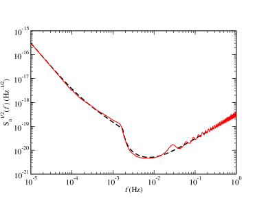
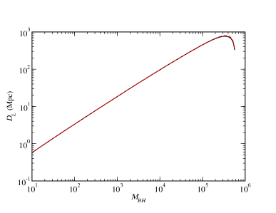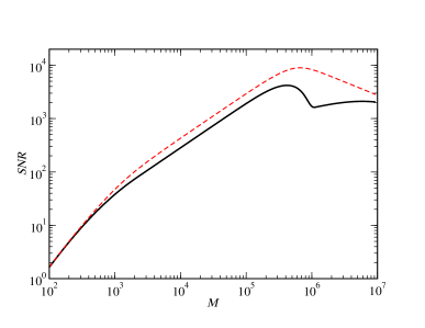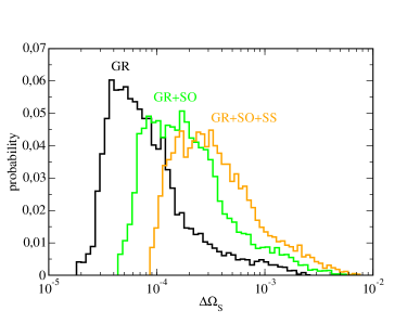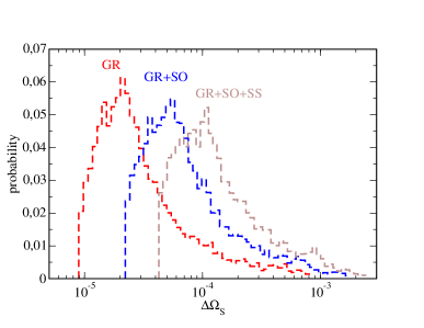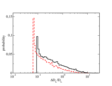
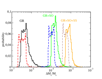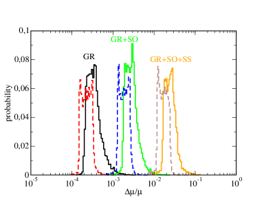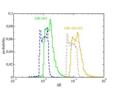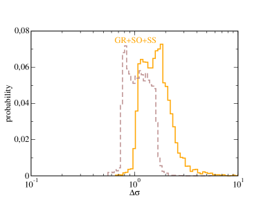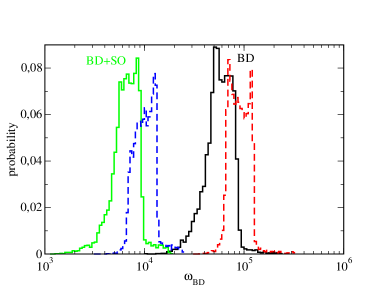
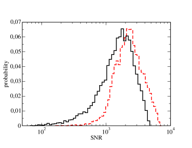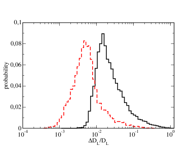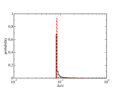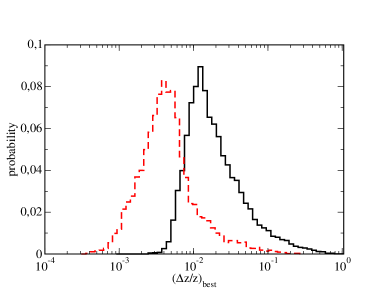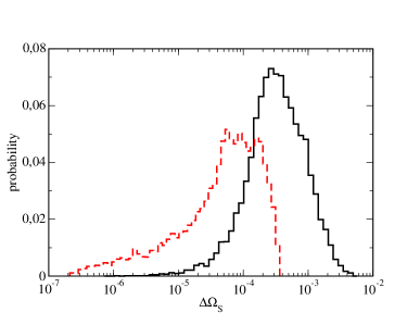
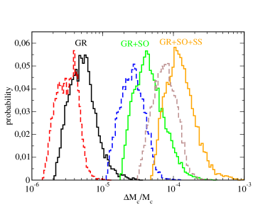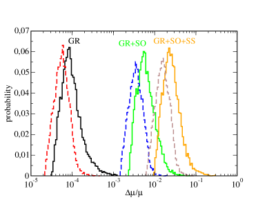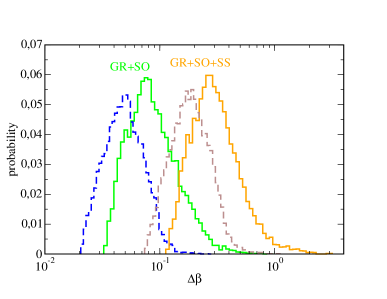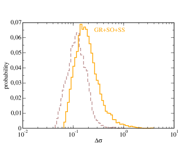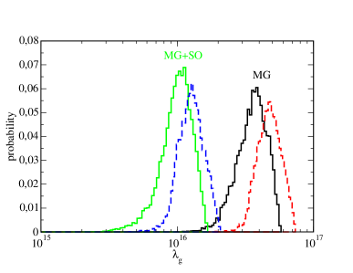
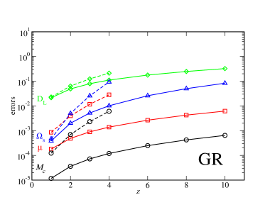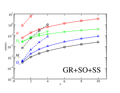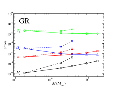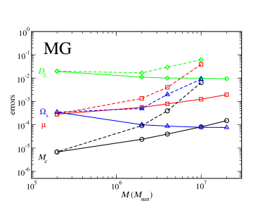Figure 1: Analytic approximation to the LISA  root noise spectral density curve used in this paper and in Ref. BC (dashed line) and the curve produced using the LISA Sensitivity Curve Generator SCG (solid line). The SCG curve has been multiplied by a factor of $\sqrt{3/20}$ to obtain an effective non-sky averaged noise spectral density (see Sec. II.3). The SCG noise curve does not include the extragalactic white dwarf confusion noise while the analytical approximation curve does.

Figure 2: Left: luminosity distances $D_{L}$ of NS-BH binaries observed with SNR=10 as a function of the black hole mass. We assume that the NS mass $M_{\rm NS}=1.4M_{\odot}$. Right: SNR for equal mass BH-BH binaries at $D_{L}=3$ Gpc as a function of the total mass. Solid lines refer to the LISA noise curve (31) used in this paper; dashed lines refer to the same noise curve without including the white-dwarf confusion noise. The “bump” in the noise curve due to white-dwarf confusion noise is responsible for the dip in the SNR for MBH binaries of masses $\sim 10^{6}M_{\odot}$.

Figure 3: Monte Carlo simulation of $10^{4}$ binaries with observed total mass $(1.4+10^{3})M_{\odot}$ in general relativity, with single-detector SNR=10, $\Omega_{\Lambda}=0.7$, $\Omega_{M}=0.3$. Top: probability distributions of the angular resolution $\Delta\Omega_{S}$ in steradians for one detector (left) and two detectors (right). In each figure, from left to right, the histograms refer to no spins, SO included, and SO and SS included. Bottom: probability distributions of $\Delta D_{L}/D_{L}$ for one detector (solid) and two detectors (dashed); $\Delta D_{L}/D_{L}$ is essentially unaffected by the inclusion of spins, so we only show histograms without the spin terms.

Figure 4: Monte Carlo simulation of $10^{4}$ binaries with observed total mass $(1.4+10^{3})M_{\odot}$ in general relativity, with single-detector SNR=10, $\Omega_{\Lambda}=0.7$, $\Omega_{M}=0.3$. Top four panels: probability distribution of the errors on the chirp mass $\Delta{\cal M}/{\cal M}$, the reduced mass $\Delta\mu/\mu$, the SO parameter $\Delta\beta$ and the SS parameter $\Delta\sigma$. Bottom panel: bound on $\omega_{\rm BD}$ when a Brans-Dicke term is included. Solid (dashed) lines refer to one (two) detector(s).

Figure 5: Monte Carlo simulation of $10^{4}$ binaries with total mass $(10^{6}+10^{6})M_{\odot}$ in general relativity, with $D_{L}=3$ Gpc, $\Omega_{\Lambda}=0.7$, $\Omega_{M}=0.3$, with no spins. Panels show probability distributions of the SNR, the distance determination error $\Delta D_{L}/D_{L}$, the redshift errors $\Delta{z}/{z}$ and $(\Delta{z}/{z})_{\rm best}$ and the angular resolution $\Delta\Omega_{S}$ in steradians. Solid (dashed) lines refer to one (two) detector(s).

Figure 6: Monte Carlo simulation of $10^{4}$ binaries with observed total mass $(10^{6}+10^{6})M_{\odot}$ in general relativity, with $D_{L}=3$ Gpc, $\Omega_{\Lambda}=0.7$, $\Omega_{M}=0.3$. Top four panels: probability distributions of the error on the chirp mass $\Delta{\cal M}/{\cal M}$, the reduced mass $\Delta{\mu}/{\mu}$, the SO parameter $\Delta\beta$, the SS parameter $\Delta\sigma$. Bottom panel: bound on the graviton Compton wavelength $\lambda_{g}$ (in km), when a massive graviton term is included. Solid (dashed) lines refer to one (two) detector(s).

Figure 7: Errors on different parameters as a function of the redshift $z$ for nonspinning BH-BH binaries with source mass $(10^{6}+10^{6})~{}M_{\odot}$ (solid lines) and $(10^{7}+10^{7})~{}M_{\odot}$ (dashed lines). We fix $\Omega_{\Lambda}=0.7$, $\Omega_{M}=0.3$. Errors are obtained by averaging results of Monte Carlo simulations of $10^{4}$ binaries and using two detectors. Left: general relativistic non-spinning binaries (GR); right: general relativistic binaries including SO and SS terms (GR+SO+SS). Circles refer to chirp mass ${\cal M}$, squares to reduced mass $\mu$, triangles to angular resolution $\Omega_{S}$ in steradians, diamonds to luminosity distance $D_{L}$.

Figure 8: Errors on different parameters as a function of the total binary mass $M$ (in solar masses) for equal-mass nonspinning BH-BH binaries. We fix $D_{L}=3$ Gpc, $\Omega_{\Lambda}=0.7$, $\Omega_{M}=0.3$. Errors are obtained by averaging results of Monte Carlo simulations of $10^{4}$ binaries and using two detectors. Left: general relativity (GR); right: massive graviton theories (MG). Solid lines assume that the LISA noise can be extrapolated down to $f_{\rm low}=10^{-5}$ Hz; dashed lines assume $f_{\rm low}=10^{-4}$ Hz. Circles refer to chirp mass ${\cal M}$, squares to reduced mass $\mu$, triangles to angular resolution $\Omega_{S}$ in steradians, diamonds to luminosity distance $D_{L}$.

Figure 9: Bound on the graviton Compton wavelength as a function of the total binary mass $M$ (in solar masses) for nonspinning equal-mass BH-BH binaries. We fix $D_{L}=3$ Gpc, $\Omega_{\Lambda}=0.7$, $\Omega_{M}=0.3$ and use both detectors. The solid line assumes that the LISA noise can be extrapolated down to $f_{\rm low}=10^{-5}$ Hz; the dashed line assumes $f_{\rm low}=10^{-4}$ Hz.

References

- (1) K. Danzmann for the LISA Science Team, Class. Quantum Gravit. 14, 1399 (1997).
- (2) P. D. Scharre and C. M. Will, Phys. Rev. D 65, 042002 (2002).
- (3) C. M. Will, Phys. Rev. D 50, 6058 (1994).
- (4) C. M. Will, Phys. Rev. D 57, 2061 (1998).
- (5) C. M. Will and N. Yunes, Class. Quantum Gravit. 21, 4367 (2004).
- (6) T. Damour and G. Esposito-Farése, Phys. Rev. D 58, 042001 (1998).
- (7) C. Cutler, Phys. Rev. D 57, 7089 (1998).
- (8) S. A. Hughes, Mon. Not. Roy. Astron. Soc. 331, 805 (2002).
- (9) N. Seto, Phys. Rev. D 66, 122001 (2002).
- (10) A. Vecchio, Phys. Rev. D 70, 042001 (2004).
- (11) S. A. Hughes and K. Menou, preprint (astro-ph/0410148).
- (12) P. L. Bender and D. Hils, Class. Quantum Gravit. 14, 1439 (1997).
- (13) L. Barack and C. Cutler, Phys. Rev. D 69, 082005 (2004). See also L. Barack and C. Cutler, gr-qc/0310125 v3, where an erroneous factor of 3/4 in the instrumental noise is corrected.
- (14) The Sensitivity Curve Generator was originally written by Shane Larson and may be found online at http://www.srl.caltech.edu/~shane/sensitivity/MakeCurve.html
- (15) E. Poisson and C. M. Will, Phys. Rev. D 52, 848 (1995).
- (16) A. Krolak, K. D. Kokkotas, G. Schafer, Phys. Rev. D 52, 2089 (1995).
- (17) B. Bertotti, L. Iess and P. Tortora, Nature 425, 374 (2003).
- (18) S. A. Hughes and D. E. Holz, Class. Quantum Gravit. 20, S65 (2003).
- (19) J. Baker and J. Centrella, astro-ph/0411616.
- (20) L. S. Finn, Phys. Rev. D 46, 5236 (1992).
- (21) L. S. Finn and D. F. Chernoff, Phys. Rev. D 47, 2198 (1993).
- (22) C. Cutler and É. E. Flanagan, Phys. Rev. D 49, 2658 (1994).
- (23) L. Blanchet, G. Faye, B. R. Iyer and B. Joguet, Phys. Rev. D 65, 061501 (2002).
- (24) L. Blanchet, T. Damour, G. Esposito-Farése and B. R. Iyer, Phys. Rev. Lett. 93, 091101 (2004).
- (25) L. Blanchet, T. Damour, B. R. Iyer, C. M. Will and A. G. Wiseman, Phys. Rev. Lett. 74, 3515 (1995).
- (26) D. N. Spergel et al., Astrophys. J. Suppl. 148, 175 (2003).
- (27) S. Finn and K. S. Thorne, Phys. Rev. D 62, 124021 (2000).
- (28) S. L. Larson, W. A. Hiscock and R. W. Hellings, Phys. Rev. D 62, 062001 (2000).
- (29) G. Nelemans, L. R. Yungelson and S. F. Portegies Zwart, Astron. and Astrophys. 375, 890 (2001).
- (30) A. J. Farmer and E. S. Phinney, Mon. Not. Roy. Astron. Soc. 346, 1197 (2003).
- (31) C. M. Will and H. W. Zaglauer, Astrophys. J. 346, 366 (1989).
- (32) M. C. Miller, Astrophys. J. 581, 438 (2002).
- (33) C. M. Will, Astrophys. J. 611, 1080 (2004).
- (34) W. H. Press, S. A. Teukolsky, W. T. Vetterling and B. P. Flannery, Numerical Recipes in Fortran, Second Edition (Cambridge University Press, Cambridge, 1992).
- (35) S. A. Hughes, (private communication).
- (36) B. Schutz, Nature 323, 310 (1986).
- (37) D. Markovic, Phys. Rev. D 48, 4738 (1993).
- (38) D. E. Holz and S. A. Hughes, astro-ph/0212218.
- (39) B. S. Sathyaprakash and B. F. Schutz, Class. Quantum Gravit. 20, S209 (2003).