Numerical integration of the Teukolsky Equation in the time domain
Abstract
We present a fourth order convergent numerical code to solve the Teukolsky equation in the time domain. Our approach is to rewrite the Teukolsky equation as a system of first order differential equations. In this way we get a system that has the form of an advection equation. This is used in combination with a series expansion of the solution in powers of time. To obtain a fourth order scheme we kept terms up to fourth derivative in time and use the advection-like system of differential equations to substitute the temporal derivatives by spatial derivatives. A local stability study leads to a Courant factor of for the nonrotating case. This scheme is used to evolve gravitational perturbations in Schwarzschild and Kerr backgrounds. Our numerical method proved to be fourth order convergent in and directions. The correct power-law tail, , for general initial data, and , for time symmetric data, was found in the simulations where the duration in time of the tail phase was long enough. We verified that it is crucial to resolve accurately the angular dependence of the mode at late times in order to obtain these values of the exponents in the power-law decay. In other cases, when the decay was too fast and round-off error was reached before a tail was developed, the quasinormal modes frequencies provided a test to determine the validity of our code.
pacs:
04.25.Dm, 04.25.Nx, 04.30.Db, 04.70.BwI Introduction
In recent years, there has been an increasing interest in numerically solving General Relativity’s (GR) field equations to provide an accurate description of the gravitational radiation generated in different astrophysical scenarios. This is due to fact that direct measure of gravitational waves will soon be possible with large interferometers such as LIGO and LISA. The astrophysical events that produce gravitational waves are among the most energetic phenomena ever seen. The best candidate for such observations are the collisions of binary black hole systems. In order to detect this gravitational radiation, accurate templates are needed, and this implies to solve the non-linear GR equations. This proved to be a very challenging task. Although in the last orbital stages (merger) of a binary black hole collision it is necessary to solve Einstein’s equations (full numerical approach), the very last part of the coalescence (close limit) the system can be considered as a single distorted black hole and can be treated with perturbation theory. Comparisons between full numerical simulations and perturbative methods show a surprising agreement. This has encouraged people to go beyond matching close limit and full numerical simulations in tandem to produce simulations that neither of each technique alone was able to do. The general method of coupling full numerical and approximate techniques is the main development of the ’Lazarus project’ Baker et al. (2000, 2001, 2002a, 2002b, 2004).
Moreover, there are physical scenarios in which the metric departure from the known static black hole solutions is always small outside the horizon. Some examples are a particle (compact object) orbiting a black hole, the propagation of gravitational waves and accretion disks near black holes. The equations evolved in the perturbative method are linear which is an advantage over the non-linear set of ten coupled general relativistic equations.
One application of perturbation theory is the propagation of waves in a curved spacetime. In this work, we will focus our study in the late time behavior of a gravitational wave in such curved spacetimes. Although the problem is not new, according to Andersson Andersson (1997) there are still some aspects for which there is no definite answer or no answers at all; like the role played by highly damped modes and the intermediate behavior of the power-law tails. Power-law tails is the name given to the last phase in the propagation of a wave in a curved background, as we will see below. The general features of the evolution of such a test field in the proximity of a black hole, as seen by a distant observer, can be divided in three stages: i) Radiation emitted directly by the perturbation source. It depends on the form of the initial field (initial data). ii) Quasinormal ringing. It depends on the parameters of the black hole. They are exponentially damped oscillations and carry part of the gravitational radiated energy in astrophysical processes like gravitational collapses. Quasinormal modes are characterized by complex frequencies . Such modes can be represented as , the real part of is the oscillation frequency and the imaginary part is the exponential damping. iii) Power-law tail. The field decays with time according the a power-law at very late times.
Most of the work on the late time radiative fall-off has been done in spherically symmetric spacetime. In this case the solution admits a decomposition in spherical harmonics. The field equations are reduced to a wave equation with a effective potential. For the Schwarzschild case this wave equation is
| (1) |
where is the tortoise coordinate
| (2) |
and
| (3) |
being the mass of the black hole.
In 1972, Price Price (1972) treated Eq. (1) as a perturbative expansion in powers of . He showed that the perturbation decays in time according to for . This situation occurs at a finite value of while , which is called timelike infinity.
Quasinormal modes and power-law tails have been studied by Leaver Leaver (1986), who analyzed the problem in the frequency domain. He found the correct late time behavior with a low-frequency approximation. Quasinormal modes can be considered as the “pure tones” of the black hole. Once excited, their damping and oscillation frequency depend only on the parameters of the black hole. Ching et. al. Ching et al. (1995) argue that the late time decay of the field can be seen as a scattering due to the spacetime curvature. This implies that the power-law behavior depends only on the asymptotic conditions of the metric. In a recent work, Poisson Poisson (2002) found that in a weakly curved spacetime the late time dynamics is insensitive to the non spherical aspects of the metric, being entirely determined by the spacetime total mass.
In Ref. Karkowski et al. (2004) it is found that the power-law tails are not an universal phenomenon as thought, but the fall-off power depend on the initial profile of the fields. While for the generic data with and the predicted Price (1972) decay goes like , when you start with an initially static field, i.e. and the predicted decay goes like .
Most of the work with the Teukolsky equation has been performed in the frequency domain (quasinormal modes, wave scattering, motion of test particles). Perturbation on the frequency domain can be reduced analytically to solve ordinary differential equations and can lead to a better understanding of the physics involved in the phenomena. Such information is much more difficult to obtain from purely numerical computations. However, in more complete treatments, the number of frequencies that one needs to consider is orders of magnitude larger than the number of points needed to resolve the direction. Furthermore, the study of quasinormal modes would require higher resolution near to resolve the tails. The resolution of the quasinormal modes is also sensitive to the spacing in frequencies. These are the argument presented by Krivan et. al. Krivan et al. (1997) in favor of a numerical treatment of perturbations using the Teukolsky equation in the time domain. Another motivation to work in the time domain is that when one tries to find a solution of the radial Teukolsky equation in the frequency domain with a source term that extends to infinity, the result is divergent. This means that the Teukolsky equation needs to be regularized when sources are present Poisson (1997); Campanelli and Lousto (1997).
The difficulty with numerical integrations of the Teukolsky equation is the linear term in on the first time derivative. Depending on the relative sign between this term and the second time derivative, it can act as a damping or anti-damping term. As described in Krivan et al. (1997), good time evolutions are achieved by writing the Teukolsky equation as a set first order differential equations system. This and other issues concerning the implementation of a fourth order algorithm are discussed in the next chapter. Motivations for a fourth order convergent algorithm are mainly, that it can reproduce the same results of a second order convergent code with less resolution. This makes the former to run faster than the later. Although in a fourth order scheme, more intense computation is needed, there is some gain in speed when equivalent resolutions, i.e. resolution that produce the same error in the solution, are used. On the other hand, if equal resolutions are used, a fourth order method will yield more accurate solutions. The price we have to pay in this case is that the fourth order method will take longer. This issues enter in consideration in gravitational wave detection, because a large number of templates need to be generated. The gain in accuracy can also be used in second order perturbation theory, since higher order derivatives of the field are needed to build up the effective source term Campanelli and Lousto (1999). This may have important applications in the ’Lazarus approach’ Baker et al. (2002a) and the radiation reaction problem of a particle orbiting a black hole.
Using the Kinnersley null tetrad:
| (4) |
where and The Newman-Penrose equations written in Boyer-Lindquist coordinates lead to the Teukolsky equation Teukolsky (1973)
| (5) |
The gravitational perturbations are recovered setting , is a parameter called spin weight. Here the quantity of interest is with and . For is , .
In vacuum, it is well know that (5) can be separated in the frequency domain, by taking . When , the functions are the spheroidal functions. When these eigenfunctions are the spin weighted spherical harmonics . The general solution can be represented as
| (6) |
In most astrophysical applications, we are interested in computing solutions that represent gravitational radiation at infinity. This information is carried by . This, together with the good asymptotic behavior of the solutions are the motivations of choosing the value to perform the time evolutions. Knowing the value of allows us to calculate the outgoing energy flux per unit time asCampanelli and Lousto (1999)
| (7) |
where and .
In the next section we explicitate the numerical techniques used to solve the Teukolsky equation starting from a review of the second order formalism developed in Ref. Krivan et al. (1997). We then derive the forth order accurate in time and space algorithm, as a natural generalization of the Lax-Wendorff algorithm. It is followed by a stability analysis that find a Courant factor of 1.5 between the time and spatial coordinate that ensures stable evolution. We finish Section II with a description of the radiative boundary conditions imposed to the field in the two radial boundaries and the angular boundary conditions imposed by the symmetry of the solution. Section III deals with the applications of the fourth order code developed. As initial data we consider an outgoing Gaussian pulse located in the far region. The fourth order convergence in both spatial variables in verified in Section III.B. We this we compute the quasinormal modes and power-law tails and an ultimately test of the code. Finally we discuss some of the consequences of the computed decay powers on the light of some discussion in the literature.
II Numerical Techniques
II.1 Review
In this work we will follow the approach used by Krivan et. al. Krivan et al. (1997). They integrate the Teukolsky equation in the time domain by rewriting it as a set a first order partial differential equations. The aim of their work is the evolution of gravitational perturbations of the Kerr spacetime. This is done for the case . This choice is due to the fact that for this particular value of spin, the solutions are bounded for both, ingoing and outgoing waves near the horizon () and at infinity (). The asymptotic behavior of the solutions of (5), for a given spin weight , representing ingoing and outgoing waves is Krivan et al. (1997), Teukolsky (1973)
| (8) |
| (9) |
The procedure of solving the Teukolsky equation is initiated by introducing the ansatz
| (10) |
where is the Kerr tortoise coordinate, defined as
| (11) |
So222Note that in the literature it is also used a different normalization for the logarithmic terms instead of it appears and respectively.,
| (12) | |||||
and is the Kerr azimuthal coordinate, defined as
| (13) |
So,
| (14) |
Now they introduce an auxiliary field defined as
| (15) |
where
| (16) |
| (17) |
This decomposes the second order differential Teukolsky equation (5) into a system of first order differential equations. The resulting equation has the form
| (18) |
where is a column vector whose components are the real and imaginary () parts of the fields and . The coefficients of the derivatives of (5) are rearranged as the elements of matrices and , given by
| (19) |
| (20) |
The remaining matrix contains the derivatives of the fields with respect to the polar coordinate , whose components are
| (21) |
The deduction of substitution (15) and the value of each element of the above matrices are given later in this chapter.
They proceed to solve the first-order system (18) using the Lax-Wendroff method Press et al. (1999). For this, (18) is written as
| (22) |
where and .
To solve the above equation in Ref. Krivan et al. (1997) it was used a grid with 8000 points for and 32 points for . The computational domain was and , with a Courant condition of .
Boundary conditions have been imposed as follows: at the horizon and outer boundary. Along the axis, or for , (the azimuthal number) odd or even, respectively.
With this settings Ref. Krivan et al. (1997) code showed stability of the order of evolution time. It was second order convergent for times , with a convergence rate higher than 1.3 for later times.
In the following sections we will concentrate in generalizing the numerical algorithm to accomplish a fourth order convergent numerical evolution, using the first-order formulation of the Teukolsky equation (18) as starting point.
II.2 Rewriting Teukolsky equation
II.2.1 Separating dependence
The Teukolsky equation is separable in the azimuthal variable for the general case of and . Furthermore, we will change the normal Boyer-Lindquist coordinates and by and , respectively. This has the advantage that approaches asymptotically to as goes to minus infinity, so the inner boundary of the computational domain is approximated very close to the horizon, but still outside the black hole.
The variable is used to improve the behavior of the coordinates near the horizon. This is a manifestation of the frame dragging effect of a rotating black hole Krivan et al. (1996).
Now we make use use of the ansatz (10) used by Krivan et. al., where they also include a factor . This is done to eliminate the increasing behavior of the solutions at infinity, according to (8). So we substitute (10) into (5), setting the source term to get vacuum space solutions. After dropping a global factor we get
| (23) | |||||
We can bring this equation into the form
| (24) |
where the ’s represent the coefficients of the derivatives. We simple multiply by . The results are:
| (25) | |||
| (26) | |||
| (27) | |||
| (28) | |||
| (29) | |||
With the Teukolsky equation written as (24), we may now proceed to transform it into an equivalent first-order differential equations system.
II.2.2 From second to first-order differential equations
A common technique to numerically solve a second-order differential equation is to rewrite it as a set of first-order differential equations and apply the appropriate methods. For cases such as the simple wave equation, getting such a first-order system is straightforward. The equation reads
| (31) |
with the velocity of propagation and . It can be written as
| (32) | |||||
| (33) |
Here is a function chosen in such a way that second derivatives are eliminated. In this case will do the job, with , and we have
| (34) | |||||
| (35) |
Now we factor out the time derivative in the first equation and the spatial derivative in the second one and we get a system of first-order equations
| (36) | |||||
| (37) |
or in matrix form
| (38) |
where the subscripts denote derivatives. Notice that it has the form of the advection equation for a system of equations
| (39) |
where is a column vector.
Trying to carry out the above procedure for the Teukolsky equation is more complicated and probably will not yield results, because it contains cross derivatives. Our approach here will be different. Recall Eq. (24), in which we set the coefficient of the second time derivative equal to one, dividing the equation by precisely this coefficient (the subscripts in the ’s do not mean differentiation with respect to the variables).
We want to write (24) as an advection equation with a source term:
| (40) |
where none of the ’s and ’s depend on . Expanding the matrix products we get two equations
| (42) | |||||
Now let and . By doing this we obtain an expression for that depends only on the derivatives of with respect to and (and some function ):
| (43) |
which is similar to (15), but has not yet been specified. We will see that with this definition, can be easily substituted and eliminated in the second equation (42). The derivatives of are
| (44) | |||||
| (45) |
Substituting (43), (44) and (45) into (42) and rearranging terms we find
| (46) | |||||
To find the value of the ’s and ’s we equate the coefficients of the derivatives of in (46) with those in (24). From the coefficient of we find that . Combining this with the coefficient of we see that :
| (47) |
This is exactly the definition of in (16). It is easy to show that the remaining equations yield the following results:
| (48) | |||||
| (49) | |||||
| (50) |
Here is defined according to (21) as the -derivative operator:
| (51) |
in the sense that it can be “factored” as and added to . Of course, an expression as (49) is not mathematically rigorous. It is rather a way to express that the equation’s angular dependence is going to be added to the source term. Furthermore, in a numerical implementation we don’t compute the value of , but the value of .
II.2.3 Splitting real and imaginary parts
Because Teukolsky equation involves complex coefficients it is necessary to treat the real and imaginary parts of the solution. Let’s define four functions and , such that
| (52) | |||||
| (53) |
and substitute them into (LABEL:eq:1st) and (42). After collecting real and imaginary parts and equating both to zero, we obtain a set of four equations. As a shorthand to denote derivatives, we use a dot for and a prime for
| (54) |
| (55) |
| (56) |
| (57) |
We can finally arrange these equations in matrix form as follows:
| (70) | |||
| (79) |
Comparing this last equation with (18) and making use of our definitions of and , equations (50) and (49), respectively; we see that our derivation yields the same structure for Teukolsky equation as that derived by Krivan et. al. Krivan et al. (1997). It is worth to comment here that although the structure of the equation is the same, the coefficients shown above do not agree completely with those of Ref. Krivan et al. (1997). The coefficients that do not agree are and the real part of , which correspond to what Ref. Krivan et al. (1997) calls and . The coefficients reported in Krivan et al. (1997) correspond exactly to the case in which the ansatz for the solution is
| (80) |
Notice that this equation does not contain the function used in (10). Another correction that needs to be done in order to recover Teukolsky equation is to set and , according to the definitions presented in Krivan et al. (1997).
Summarizing, the coefficients used in this work, using the ansatz (10) are
| (81) | |||||
| (82) | |||||
| (83) | |||||
| (84) | |||||
| (85) | |||||
| (86) |
II.3 Derivation of the 4th order algorithm
Let’s assume that is a continuously differentiable function and that its derivatives in both and exist up to order four in some given interval. This function satisfies a differential equation of the form
| (87) |
where is a constant and the subscripts represent first derivatives with respect to and respectively. The Taylor expansion in for is
| (88) |
Here and its derivatives are evaluated at some given point . Now we can use eq. (87) to replace the time derivatives by spatial derivatives, using the fact that , and so on. Thus we have
| (89) | |||||
If we truncate this series, taking terms up to we will obtain the Lax-Wendroff scheme, which is second order accurate in space and time. Introducing the usual discrete notation for and using a second order accurate approximation for derivatives we have Kincaid and Chaney (2002)
| (90) | |||||
where .
In order to have a fourth order accurate scheme, we truncate the Taylor expansion of including terms up to and using the differential equation (87) to replace time derivatives by space derivatives. Furthermore, we use a fourth order finite difference scheme (see appendix A) to approximate spatial derivatives. Proceeding in this way we have
| (91) |
Notice how the dependence on the discretization parameters and appears as powers of .
II.4 Stability analysis
We apply now a von Neumann stability analysis to the previous scheme. This analysis is local, which means that we assume that the coefficients of the finite difference equation vary slowly in space and time such that they can be considered to be constant. In our case, these coefficients do not depend on time. We say that the method is stable if the scheme is stable for every constant value of the coefficients in their range Sewell (1988). The idea is to expand the solution of the difference equation in its eigenmodes , where is a real wave number. The time dependence of these modes is a succession of powers of some complex number , called amplification factor. With this, we say that the difference equation is stable if , for a given value of . The eigenmodes of the difference equation (91) can be written as Press et al. (1999)
| (92) |
where is a complex quantity and is a real wave number. Substituting (92) into (91) we get a first grade polynomial in . After some algebra we get
or
This is a periodic function with a period of . For the scheme to be stable it has to satisfy the stability condition
| (95) |
Although we can find analytic solutions for this equation, just to present them here would occupy several pages. Rather than analytic solutions, we are interested in some interval of values for , such that our fourth order method is stable. The behavior of as a function of is shown in Fig. 1 for some values of . With certainty, we can conclude that is less than 1 for . This implies that the Courant condition for this case is
| (96) |
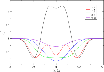
This value is greater than that required by the Lax-Wendroff method and many others. This can be understood by expanding the amplification factor in series of . In practice must be small enough to correctly approximate the continuous differential equation. This means that for modes corresponding to small values of we can expand (LABEL:eq:xi1) in a power series of . That is
| (97) |
It is interesting to compare this with the corresponding series expansion of for the Lax and Lax-Wendroff methods. For the Lax method we find Press et al. (1999)
| (98) |
and for the Lax-Wendroff method we have
| (99) |
We can see that our fourth order method has a sixth order dependence of , which means that mode damping effects become relevant for much higher values of , making this method more accurate. The generalization of the scheme to two dimensions is illustrated in the last subsection. In this case the situation is more complicated because we are taking first and second derivatives in the direction. We were not able to find an analytic Courant factor that took into account the direction. From numerical experiments we verify that the Courant condition used in Krivan et al. (1997) was reliable in our case too. Thus, as a rule of thumbs, we always kept .
II.5 Boundary conditions
II.5.1 Radial boundary conditions
We use Sommerfeld boundary conditions at radial infinity and at the event horizon. When one uses the tortoise coordinate the event horizon is reached when . In practice, it turns that setting is a good approximation. For this value we have . At the inner boundary, the condition is that of an ingoing wave
| (100) |
At the outer boundary, the appropriate condition is that of an outgoing wave
| (101) |
In order to make this conditions compatible with our fourth order integration scheme, we take higher derivatives of (100) and (101). The idea is again, to substitute the time derivatives of the Taylor expansion (88) by means of the boundary conditions above. The results are summarized in table 1.
| Inner boundary | Outer boundary |
|---|---|
The implementation of boundary conditions is straightforward when a second order scheme is employed. This is due to the fact that we only need up to second order spatial derivatives and its stencil demands only 3 points333For centered finite differences, a second order accurate formula needs two points to compute first derivatives and three points for second derivatives.. On the other hand, the case of a fourth order accurate expression for spatial derivatives needs two more points for the first derivative and seven points for the fourth derivative, see appendix A. So, in this case, the way we implemented the radial boundary conditions is to use off-centered expressions to compute the spatial derivatives, when needed. Assuming a computational grid of points in the direction, labeling the points from 0 to , table 2 shows the points for which off-centered spatial derivatives are used.
| Off-centered derivatives | used at points |
|---|---|
| 1, | |
| 1, 2, , |
As to the auxiliary field , defined in (15), its boundary condition follows directly from its definition and from (100) and (101). Once we know the boundary values for , the value for at the inner boundary is
| (102) | |||||
| (103) |
where we have used (100) and is given by (16). In a similar way, the outer boundary condition is
| (104) |
II.5.2 Angular boundary conditions
These are imposed along the rotation axis, i.e. at and . The boundary condition depends on the particular azimuthal mode (see equation (10)) chosen for the evolution, it can be stated as
| for | (105) | ||||
| for | (106) |
This conditions come directly from the behavior of the solution in the direction. At the same time it is precisely this behavior what we use in order to implement the appropriate boundary conditions. The solutions for which is even, have even parity about both, and . On the other hand, the solutions with odd , have odd parity about and , i.e.
| for | (109) | ||||
| for | (113) |
To take advantage of this property we need to use a staggered grid in the direction. By doing this we also avoid the inherent difficulties of evaluating expressions in which is present, (like the last term of Teukolsky equation (5)) since this function is not finite neither at nor . In a staggered grid, the values for and are always located exactly between two grid points. The points to the left (right) of () are considered as “ghost zones”, because are used just to implement the boundary conditions. In our fourth order method, we need four ghost points. Two before the first point immediately after and two more after the point immediately before , as shown in Fig. 2. Our grid has points in the direction, the first two and last two points are ghost zones. In this way we can always use a centered formula to compute the derivatives in the direction. Notice that if we are using a second order accurate approximation, we only need one ghost point at each end of the grid. The values of the ghost zones are updated according to (LABEL:eq:BCth0) and (LABEL:eq:BCthpi).

These properties of the solutions are a direct consequence of the spherical harmonics behavior (when the spin parameter ) and the spin weighted spherical harmonics (when ).
II.6 Notes on implementation
We mention here some implementation details of equation (18), which for convenience will be written as444We use lower case bold face to denote vectors and upper case bold face to denote matrices.
| (115) |
As stated above, the main idea has been always to substitute the time derivatives in the Taylor expansion (88) by spatial derivatives using our differential equation (115). Calling and , all time derivatives needed are:
| (116) | |||||
| (117) | |||||
| (118) | |||||
| (119) |
Here we have used the fact that none of the coefficient of the Teukolsky equation are time dependent and that partial derivatives commute.
The four time derivatives above could be computed using just the finite differences formula for the first derivative in . Once we know we can numerically substitute this result to get the second time derivative and so on. The problem with this procedure is that because of the exclusive use of the first derivative formula; at the end, we will not have a fourth derivative with the accuracy shown in appendix A. It still will be fourth order accurate but using the first derivative formula four times will propagate more error than that of the fourth order accurate finite differences formula. The same holds for the other derivatives. The approach we took was to compute all time derivatives directly from the coefficients of the evolution equation, and the value of the fields at every time step. Of course, this implies much more larger expressions to compute time derivatives, because now we have to algebraically substitute one time derivative into the other. Carrying out such a substitutions we find:
| (120) | |||||
| (121) | |||||
| (122) | |||||
| (123) | |||||
To clarify the equations, we have used “primes” to denote differentiation with respect to .
There is one final issue, worth mentioning here. Notice that there are still some products in which the time derivatives of and itself appear explicitly. All of these products involve multiplication with . Neither the time derivatives nor are algebraically substituted in these products because and contains the derivatives operator. Instead of expanding further derivatives, we chose to numerically substitute the time derivatives of and itself into these products. We use the term “numerically substitute” in the sense that each time derivative is calculated and stored in the memory of the computer, further computation makes use of the stored values.
Such a procedure gives good results as shown in the next section.
III Results
III.1 Initial data
In all runs, initial data with compact support was used. The function used was a Gaussian bell centered at , in the direction and some mode dependence in the direction. Thus, for we have
| (124) |
where represents the dependence as spherical harmonics or the spin weighted spherical harmonics ; for or , respectively. Table 3 shows the dependence of the first four spherical harmonics and spin weighted spherical harmonics.
| -mode | ||
|---|---|---|
| constant | – | |
| – | ||
III.2 Fourth order convergence
Convergence was tested in both and directions. The method to assess convergence was to compare three runs for the same initial data but different resolutions. If we want to measure convergence in the direction, we keep resolution fixed; while we vary resolution. The same holds in the case of assessing convergence. The way of varying resolutions is such that they keep the same ratio. If we call this resolutions fine, medium and coarse; they satisfy:
| (125) |
where is some positive number. In practice, this ratio was taken to be 1.5 or 2. Each time the resolution is increased, the numerical solution must converge to the true solution. The numerical solution will have an error of the order of , then we can say that
| (126) | |||||
| (127) | |||||
| (128) |
where is a constant. From these relations it is easy to verify that
| (129) |
This means that when plotted together, and must lie on top of each other and that will indicate that our numerical scheme is fourth order convergent. The same applies in the case of .
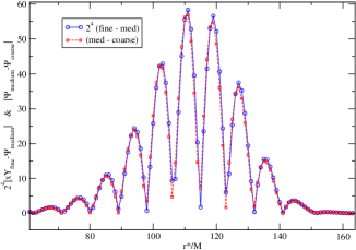
Starting with the direction, Figs. 3-5 shows fourth order convergence. The simulation parameters are (in all runs the black hole mass is taken as and the Courant factor is 0.5):
| domain: | |
|---|---|
| grid size : | |
| resolution: | , |
| physical parameters: | |
| initial data: | ingoing Gaussian pulse |
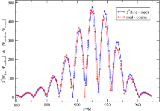
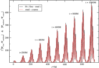
Figure 3 shows the differences (129) in absolute value. It corresponds to the instant . By this time the initial pulse has bounced off the potential barrier and has reached a maximum amplitude of . A rough estimation indicates an error of 0.08% at the highest amplitud. Fig. 4 shows the same phase than the previous one but at . The error has increased now to . A carefull examination of Fig. 4 shows that the difference between the two lines is more notorious than in Fig. 3. That means that the convergence ratio is less than 4, but it is still consistent within a ratio of 3.95. Fig. 5 shows the same phase of the previous two graphs at different time steps. It is very clear that the relative error increases linearly with time.
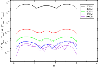
As for the convergence in the direction, a minor problem needs to be solved before computing the differences of the three numerical solutions. The problem is that the implementation of a staggered grid in causes that the discrete set of values were completely different when resolution is changed. This fact is illustrated in Fig. 6. Therefore, in order to assess convergence, we used a sixth order Lagrange polynomial to interpolate the solution obtained with the medium and finer resolutions at the values of the coarse one. Having done that, Fig. 7 shows fourth order convergence for a fixed value of . The simulation parameters are still the same but this time and , i.e. the ratio . The amplitude decreases as the wave passes by. The graph shows different snapshot at intervals of . Convergence is lost when round-off error is reached.

Other test performed to check the validity of the numerical solutions was evolving the initial data of a known analytic function. This function does not need to be a solution of the Teukolsky equation, it could be any smooth function in and , provided that the corresponding source term is added to the evolution equations. The idea is the following: let’s call the “Teukolsky operator” so that is the Teukolsky equation (23). If we choose an arbitrary smooth function , the result of applying the operator will be
| (130) |
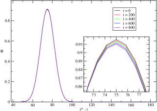
If we add the source term to the evolution equations and give the initial data as and our code should reproduce the function . In Fig. 8 we show the result of such a test. We set the function as a Gaussian pulse (in and ), traveling in the increasing direction of . Our code reproduce the analytic function with high accuracy. There is some damping in the amplitude of the pulse due to numerical dispersion; however, this effect appears at very late times.
III.3 Power-law tails
The main application of this work is to accurately compute the power-law falloff in the gravitational perturbations evolution. In the following results the observation point is located at M and . The highest resolution used was M, and the lowest one was M, . Variation of the resolution in those intervals was done in order to verify convergence, although the lowest resolution was not enough in cases where the profile presents several oscillations. Computationally, the determination of power-law tails is a challenging problem, because the amplitude of the wave decays exponentially during the quasinormal ringing and as an inverse power of time during the tail phase. This means that we are working with very small numbers that eventually reach round-off error, due to the finite precision of the computer processor. This posses some difficulties when we try to determine the exponent of the power-law. Recall that at very late times, for a finite value of (timelike infinity), the amplitude of the field goes as
| (131) |
In principle, finding this exponent should not be a problem since the field is proportional to a power of the time . Thus, a simple power fitting of the form (where and are constants) would be just enough. The problem with this procedure is that (131) is the very last stage in the evolution of the perturbation. In practice, we are not able to evolve the perturbations for such a long time, due to the finiteness of computational resources555In our case this finiteness is precisely RAM memory. This is because the outer boundary condition is not perfect and after some finite time, part of the initial pulse is reflected back. To delay the arrival of this reflection the outer boundary must be far away from the observation point, which means a large computational domain; in other words: more RAM memory.. So we analyze the field just from the moment the tail phase begins until the moment the solution reaches round-off error. During this period, the field falloff is governed also by powers of time smaller than Scheel et al. (2004):
| (132) |
which means that the exponent of reaches in an asymptotic way. Taking this fact in consideration, we compute the “local power index” Burko and Ori (1997) defined as , and use a linear fit (least-squares) such that
| (133) |
where the ’s are constants.
The least-squares fit yields good results when the local power index (that is computed taking numerical derivatives of ) is taken in a large interval over which its oscillations are small. This behavior of is illustrated in Fig. 9. For times longer than those shown in this plot, the oscillation of becomes larger and the meaning of the local power index is lost.
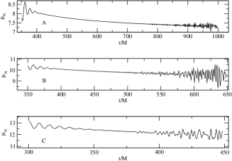
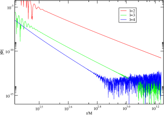
We notice that the larger the value of the shorter the interval of validity for . This is due to the fact that for larger values of , the power-law exponent is bigger (in absolute value), making the field to decay very fast reaching round-off error earlier. Fig. 10 shows this behavior for , and different values of . A closer examination of Figs. 9 and 10 reveals that the oscillations in start some time before round-off error appears. The origin of such behavior is attributed to the accumulated numerical error that increases as the evolution progresses. This oscillations are magnified in Fig. 9 due to the numerical time derivatives of the field .
| predicted | |||||
| 2 | 0 | 7 | 6.866 0.004 | 7.00 0.03 | 7.18 0.01 |
| 2 | 1 | 6.87 0.01 | 7.01 0.03 | 7.177 0.003 | |
| 2 | 2 | 6.87 0.01 | 7.04 0.06 | 7.180 0.005 | |
| 3 | 0 | 9 | 8.64 0.04 | 8.9 0.3 | 9.24 0.02 |
| 3 | 1 | 8.62 0.04 | 8.9 0.2 | 9.22 0.02 | |
| 3 | 2 | 8.62 0.02 | 8.9 0.1 | 9.23 0.01 | |
| 3 | 3 | 8.65 0.04 | 9.1 0.2 | 9.23 0.02 | |
| 4 | 0 | 11 | 10.1 0.7 | 11.3 0.7 | 11.23 0.04 |
| 4 | 3 | 9.9 0.1 | 10.7 0.7 | 11.06 0.04 | |
| 4 | 4 | 10.2 0.1 | 11.5 0.5 | 11.31 0.03 |
| 2 | 0 | 460 | 220 | 76278 | 144986 | |||
| 2 | 1 | 440 | 234 | 71298 | 151267 | |||
| 2 | 2 | 439 | 198 | 82955 | 150505 | |||
| 3 | 0 | 577 | 314 | 61318 | 134175 | |||
| 3 | 1 | 583 | 346 | 55274 | 135607 | |||
| 3 | 2 | 580 | 306 | 64049 | 134996 | |||
| 3 | 3 | 569 | 173 | 92460 | 132637 | |||
| 4 | 0 | 798 | 502 | 91111 | 145278 | |||
| 4 | 3 | 885 | 253 | 112895 | 158033 | |||
| 4 | 4 | 783 | 136 | 164384 | 140118 | |||
Table 4 shows the results a linear fit of the form (133) for the case and different values of and . The fourth column shows the value of the exponent using a fitting curve of the form . The fifth column corresponds to a fitting curve and the sixth column takes in consideration only a quadratic correction in , i.e. . The uncertainty is the statistically computed error for the parameter in the fitting. This quantity is greater in the case of corrections because there are three constants to be adjusted. The exponents are in agreement with the expected value . The agreement is better for than for and for the correction than for the and one. In two cases (, ), the duration of the tail was not enough to determine the exponent. The interval chosen to make the curve fitting was the largest one that starts after the quasinormal ringing and ends before the amplitude of the oscillations got too high in a way that it could bias the result. In table 5 we show the values of the coefficients and for the three different fitting functions. It is very interesting to notice that the weight of the term is greater than that of by a factor of at least 200. This result supports, to some extend, the model proposed by Poisson Poisson (2002) for the radiative falloff of a scalar field in a stationary, asymptotically flat and weakly curved spacetime. He shows that the first correction to the power-law tail is of order . Our observation point is located at and it is not far enough from the black hole to say that it is in the asymptotically flat region.
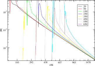
To find out the behavior in the asymptotically flat region we did similar evolutions for the scalar case and . Tables 6 and 7 show the power law tail computed at different observation points in the equatorial plane. In the first one the initial data was an outgoing Gaussian pulse centered at M. In the second one, initial data has the same initial shape but the pulse has zero velocity, i.e. it is time symmetric. We see that the power law tail is 4 instead of 3 for time symmetric initial data. The fact that the fitting to a function of order yields tails closer to the predicted value for distant observer supports Poisson’s formula. Figure 11 show the exponential fall off at different distances from the black hole as a function of time. All them approach asymptotically to the theoretically known value.
| observ | |||
|---|---|---|---|
| 20 | 2.969 | 2.951 | 3.001 |
| 50 | 2.965 | 2.951 | 3.001 |
| 150 | 2.922 | 2.951 | 3.005 |
| 250 | 2.825 | 2.967 | 3.025 |
| 350 | 2.649 | 2.928 | 3.095 |
| 450 | 2.474 | 2.807 | 3.190 |
| 550 | 2.595 | 2.939 | 3.104 |
| 650 | 2.377 | 2.906 | 3.234 |
| observ | |||
|---|---|---|---|
| 20 | 3.959 | 4.005 | 4.001 |
| 50 | 3.950 | 4.005 | 4.002 |
| 150 | 3.859 | 3.999 | 4.019 |
| 250 | 3.652 | 3.981 | 4.079 |
| 350 | 3.601 | 3.979 | 4.084 |
| 450 | 3.296 | 3.941 | 4.219 |
| 550 | 3.419 | 3.961 | 4.143 |
| 650 | 3.128 | 3.921 | 4.291 |
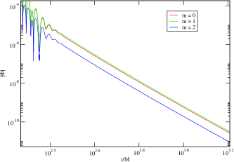
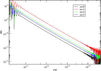
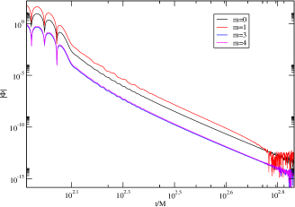
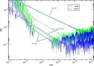
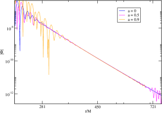
Figure 12 shows the evolution for the multipole for different values of . In these cases there is no presence of round-off error because it has the slowest decay rate, . In Fig. 13 we see the same situation as above but with . The power-law has a behavior . Round-off error appears at . Finally in Fig. 14 round-off error appears approximately at the same value of as in the previous case. We notice that the quasinormal ringing is practically inexistent. In all the runs we use outgoing initial data as prescribed in (124).
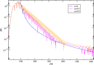
So far we have been considering power-law tails for the case of a non-rotating black hole (). Fig. 15 shows the power-law tails for the case in which . We can see that for these values of the duration of the tail is too small. Doing a nonlinear fitting for the case , we found a tail of . For the other cases, this very short tail phase is not enough to tell with certainty the power-law exponent; besides, the tail has still some small oscillation in that time interval. To verify the effects of a Kerr spacetime in the evolution of the gravitational perturbations, the frequencies of the quasinormal ringing are useful; as shown in the next section.
III.4 Quasinormal modes
We compute the quasinormal modes frequency for the cases shown in Fig. 15, which correspond to the Kerr spacetime (table 8). The case agrees with the known frequencies Seidel and Iyer (1990); Kokkotas (1991) with an error less than . The cases and have frequencies similar to the multipole. We also compute these frequencies for the case of a Schwarzschild spacetime (table 9). In this case, the frequency values agree with the predicted ones Leaver (1985); Giammatteo (2003); Fröman et al. (1992) within a 0.1 to error. In the cases for , the numerical evolution was not able to render quasinormal ringing. For , angular mode conversion to the lowest allowed multipole is present. The case , presents an irregular oscillation and the real part of the frequency and cannot be trusted. That is the reason why it is not shown here.
| computed M | predicted M | ||
|---|---|---|---|
| 2 | 0 | ||
| 2 | 1 | ||
| 3 | 0 | NA | |
| 3 | 1 | ||
| 4 | 0 | NA | |
| 4 | 1 | NA |
| M | predicted M | ||
| 2 | 0 | ||
| 2 | 1 | ||
| 2 | 2 | ||
| 3 | 0 | ||
| 3 | 1 | ||
| 3 | 2 | ||
| 3 | 3 |
III.5 Fourth order versus second order
We could say that the advantage of using a fourth order convergent code is that we can achieve the same results of the second order one with less resolution. In other words, the same degree of accuracy can be obtained with both approaches in the same computational domain but the second order one will need more points. Quantitatively, we can compare the error in the solution for both cases. This error is the difference between the true solution and the numerical solution for a given resolution. If we denote this quantity by , where is the grid spacing then we have:
| (134) |
where is a constant and is the order of accuracy. If we equate the errors for and , the relationship between resolutions is
| (135) |
If in the fourth order method, then the equivalent resolution in the second order one is approximately 10 times bigger! i.e. . This implies that in a one dimensional problem the number of points is also 10 times bigger. If a two dimensional problem is considered then the second order grid should contain 100 times more points than that of the fourth order method, to get the same error in the solution.
A feature of the finite differences methods is that according to (134), if we increase resolution by some factor the error is reduced by a factor . Thus each time we double resolution, the error decreases by a factor of 4 in the second order method and by 16 in the fourth order method.
The above considerations put the fourth order method in a better position than the second order one but, as we said in the introduction, the price we have to pay is running time. Given a resolution , the fourth order method will find a more accurate solution than the second order one. The time that the fourth order method will take will be longer because there are much more calculations to be done. In order to determine if the gain in a smaller grid is greater than the loss in running time, we did some numerical experiments. The running time is given approximately by
| (136) |
where is the running time at resolutions and . Fixing and , min in the case of the fourth order method; and min for the second order one (we used a Pentium 4 CPU 2.4GHz). These times correspond to the gravitational case , in an interval M being the simulation time 1600 M. In this simulation, the fourth order method gave very good results whereas the second order one becomes unstable around M. In order to obtain the same result (power-law tail) than the fourth order one, it was necessary the increase the resolution four times in both directions. This implies that now, the running time for the second order method is min. This time is 14 times larger than that corresponding to the fourth order method. So we definitely have a gain in speed, when the errors in the numerical solutions (for both methods) are kept equal.
As to the RAM memory, table 10 gives information about the amount of memory used in function of the grid size (). These values depend on the coding details of the algorithm. In this kind of problem, computer memory is not a crucial factor as it is the speed.
| RAM memory [Mb] | running time [hrs] | |||
|---|---|---|---|---|
| 2nd order | 4th order | 2nd order* | 4th order | |
| 19 | 22 | 0.06 | 0.25 | |
| 64 | 71 | 0.48 | 2 | |
| 236 | 249 | 3.73 | 16 | |
IV Conclusions
The main goal of this research has been to implement a stable fourth order accurate method to numerically integrate the Teukolsky equation in the time domain. In order to verify and evaluate the efficacy of our fourth order method, we have reproduced the main known results, i.e. power-law tails and quasinormal ringing. Power-law tails is a subject in which there are still unsolved questions concerning the late time behavior of the perturbations and its dependence on the coordinates and the initial data Poisson (2002). We addressed some of these issues here and others are left for future research. Among the formers, we studied the case of an initial pulse with an initial configuration such that and . We have been able in this case that the late time behavior agrees well with the predicted Karkowski et al. (2004) decay . We have also confirmed numerically that for an observer located far away from the hole we see the predicted Poisson (2002) correction to the power law as .
The fourth order method implemented in this work has shown to be convergent and stable in all runs we did. The ansatz proposed by Krivan et. al. Krivan et al. (1997) effectively removes the growing in time of the field, a feature that is expected from the asymptotic behavior of the solutions. When carrying out our calculation, we notice that the coefficients of the Teukolsky equation reported in Krivan et al. (1997) do not correspond to those we got when the ansatz proposed is used. Instead, they correspond to an ansatz without the factor (see eq. (10)). We also verify that the formulation of Teukolsky equation as a system of first order differential equations is a powerful technique because it allows to express the first time derivative in function of the spatial derivatives. The resulting system of equations has the form of the advection equation. That was the key idea that allowed us to implement a fourth order method to solve the equation: expand the solution in power series of time keeping terms up to fourth order and then use the differential equation to substitute the time derivatives by spatial derivatives. Using this procedure, a higher order method could be developed in a straightforward manner. The stability analysis provided a limiting value of the Courant of 1.5 below which we can perform stable evolutions.
The time evolutions carried out with the fourth order method yielded accurate results even when relatively low resolutions were used. The lowest resolution was , for the , case. The highest resolution used was and , for the multipole. In finite difference methods the resolution is chosen in such a way that the details in the profiles of the functions involved in the calculations can be accurately approximated. For higher values of , the -dependence has more oscillations in its domain therefore more points are needed to find a reliable solution. The more oscillations or narrow peaks a function has the more resolution we need. This comes from the fact that those functions have derivatives whose values oscillate rapidly and higher derivatives vary even faster. If the resolution is not good enough the effect is a “numerical mode mixing”, that has nothing to do with the physical model, but with the numerical aspects of the implementation. This mode mixing acts like if we were evolving the waves in a Kerr background, where physics tells us that angular mode mixing is expected. This unwanted effect cannot be easily detected when in the simulations. Therefore it is absolutely necessary to verify that this effect is not present when we evolve in the Schwarzschild background, where the physical mode mixing does not happen. This may explain some discrepancy on the computed power-law exponent decay appeared in the literature.
For table 8 shows clearly that for the mode mixing acts bringing down the quasinormal frequencies close to that of the . The same effect is observed in the tails power, although it is more difficult to prove (See Fig. 15).
Boundary conditions were not an issue of concern in this research. The radial inner boundary was not a problem because the field decays exponentially near that region. The radial outer boundary always reflects part of the wave. The immediate solution is to push this boundary far away such that this reflection does not interfere in the region of interest. A refinement of the boundary conditions will be needed when a large computational domain can not be used in favor of higher resolutions.
We have a reliable computational tool to explore several interesting problems concerning first order perturbations. We expect to shed some light on problems like the late time behavior of gravitational and scalar fields in a Kerr background. This is a problem that has been studied both analytically and numerically in recent years and there are still questions to be answered. Further research could include the problem of the orbiting particle around a black hole and the close limit approximation in the problem of two colliding black holes Lousto (2001).
Acknowledgements.
We are very grateful to E. Poisson for useful discussions on power-law tails, and to K. Kokkotas for making available unpublished values of the Quasinormal frequencies for rotating black holes. We also gratefully acknowledge the support of the NASA Center for Gravitational Wave Astronomy at The University of Texas at Brownsville (NAG5-13396) and also to NSF for financial support from grants PHY-0140326 and PHY-0354867.Appendix A Fourth order accurate derivatives
This are the formulas to compute fourth order accurate derivatives using finite differences. Those which are centered have always less truncation error than the corresponding off-centered ones. In all of them, is the size of the step and . We neglect term of powers higher than four.
-
•
First derivative
-
–
centered:
(137) -
–
off-centered (1 point):
(138) -
–
off-centered (2 points):
(139)
-
–
-
•
Second derivative
-
–
centered:
(140) -
–
off-centered (1 point):
(141) -
–
off-centered (2 points):
(142)
-
–
-
•
Third derivative
-
–
centered:
(143) -
–
off-centered (1 point):
(144) -
–
off-centered (2 points):
(145) -
–
off-centered (3 points):
(146)
-
–
-
•
Fourth derivative
-
–
centered:
(147) -
–
off-centered (1 point):
(148) -
–
off-centered (2 point):
(149) -
–
off-centered (3 points):
(150)
-
–
References
- Baker et al. (2000) J. G. Baker, B. Brügmann, M. Campanelli, and C. O. Lousto, Class. Quant. Grav. 17, L149 (2000), eprint gr-qc/0003027.
- Baker et al. (2001) J. G. Baker, B. Brügmann, M. Campanelli, C. O. Lousto, and R. Takahashi, Phys. Rev. Lett. 87, 121103 (2001), eprint gr-qc/0102037.
- Baker et al. (2002a) J. G. Baker, M. Campanelli, and C. O. Lousto, Phys. Rev. D65, 044001 (2002a), eprint gr-qc/0104063.
- Baker et al. (2002b) J. G. Baker, M. Campanelli, C. O. Lousto, and R. Takahashi, Phys. Rev. D65, 124012 (2002b), eprint astro-ph/0202469.
- Baker et al. (2004) J. Baker, M. Campanelli, C. O. Lousto, and R. Takahashi, Phys. Rev. D69, 027505 (2004).
- Andersson (1997) N. Andersson, Phys. Rev. D 55, 468 (1997).
- Price (1972) R. Price, Phys. Rev. D 5, 2419 (1972).
- Leaver (1986) E. Leaver, Phys. Rev. D 34 (1986).
- Ching et al. (1995) E. Ching, P. Leung, W. Suen, and K. Young, Phys. Rev. D 52 (1995).
- Poisson (2002) E. Poisson, Phys. Rev. D 66, 1 (2002).
- Karkowski et al. (2004) J. Karkowski, Z. Swierczynski, and E. Malec, Class. Quant. Grav. 21, 1303 (2004), eprint gr-qc/0303101.
- Krivan et al. (1997) W. Krivan, P. Laguna, P. Papadopoulos, and N. Anderson, Phys. Rev. D 56, 3395 (1997).
- Poisson (1997) E. Poisson, Phys. Rev. D55, 639 (1997), eprint gr-qc/9606078.
- Campanelli and Lousto (1997) M. Campanelli and C. O. Lousto, Phys. Rev. D 56, 6363 (1997).
- Campanelli and Lousto (1999) M. Campanelli and C. O. Lousto, Phys. Rev. D 59, 124022 (1999).
- Teukolsky (1973) S. Teukolsky, The Astrophysical Journal 185, 635 (1973).
- Press et al. (1999) W. H. Press, S. A. Teukolsky, W. T. Vetterling, and B. P. Fannery, Numerical Recipies in C (Cambridge University Press, 1999).
- Krivan et al. (1996) W. Krivan, P. Laguna, and P. Papadopoulos, Phys. Rev. D 54, 4728 (1996).
- Kincaid and Chaney (2002) D. Kincaid and W. Chaney, Numerical Analysis: Mathematics of Scientific Comuting (Brooks/Cole, 2002).
- Sewell (1988) G. Sewell, Finite Differences, Finite Elements and PDE2D. (The Numerical Solution of Ordinary and Partial Differential Equations) (Academic Press (out of print), 1988).
- Scheel et al. (2004) M. A. Scheel et al., Phys. Rev. D 69, 104006 (2004).
- Burko and Ori (1997) L. Burko and A. Ori, Phys. Rev. D 56, 7820 (1997).
- Seidel and Iyer (1990) E. Seidel and S. Iyer, Phys. Rev. D 41, 374 (1990).
- Kokkotas (1991) K. D. Kokkotas, Class. Quantum Grav. 8, 2217 (1991).
- Leaver (1985) E. Leaver, Proc. R. Soc. London A402, 285 (1985).
- Giammatteo (2003) M. Giammatteo, gr-qc/0303011 (2003).
- Fröman et al. (1992) N. Fröman, P. O. Fröman, N. Andersson, and A. Hökback, Phys. Rev. D 45, 2609 (1992).
- Lousto (2001) C. O. Lousto, Phys. Rev. D 56, 6363 (2001).