Statistical mechanics and the description of the early universe
II. Principle of detailed balance and primordial 4He formation

M. E. Pessaha,b and Diego F. Torresb
aFacultad de Ciencias Astronómicas y Geofísicas, UNLP, Paseo del Bosque s/n, 1900, La Plata, Argentina
bInstituto Argentino de Radioastronomía, C.C.5, 1894 Villa Elisa, Buenos Aires, Argentina
Abstract

If the universe is slightly non-extensive, and the distribution functions are not exactly given by those of Boltzmann-Gibbs, the primordial production of light elements will be non-trivially modified. In particular, the principle of detailed balance (PDB), of fundamental importance in the standard analytical analysis, is no longer valid, and a non-extensive correction appears. This correction is computed and its influence is studied and compared with previous works, where, even when the universe was considered as an slightly non-extensive system, the PDB was assumed valid. We analytically track the formation of Helium and Deuterium, and study the kind of deviation one could expect from the standard regime. The correction to the capture time, the moment in which Deuterium can no longer be substantially photo-disintegrated, is also presented. This allows us to take into account the process of the free decay of neutrons, which was absent in all previous treatments of the topic. We show that even when considering a first (linear) order correction in the quantum distribution functions, the final output on the primordial nucleosynthesis yields cannot be reduced to a linear correction in the abundances. We finally obtain new bounds upon the non-extensive parameter, both comparing the range of physical viability of the theory, and using the latest observational data.


1 Introduction

Primordial nucleosynthesis provides an interesting testing arena where to analyze the viability of physical theories, particularly, of the statistical description. It is in this epoch where the earliest bounds upon a given theory with cosmological influence can be imposed. Thermal processes (see Ref. [1], hereafter referred as Paper I) are non-trivially modified by a non-extensive correction to quantum distribution functions. Then, different abundances of light elements are a possible outcome.

Some of the predictions for primordial nucleosynthesis in a non-extensive setting have been analyzed before by some of us, using the asymptotic approach of the quantum distribution functions, see Refs. [2, 3]. Here, instead, we shall consistently continue within the formalism given in Paper I. Since this approach is simpler, we shall obtain analytical results far beyond the point where previous works have reached, see for instance Ref. [3, 4]. Together with Paper I, we shall then provide a complete history of the early universe, accordingly modified taking into account a non-extensive setting. In this paper, we shall focus on the study of the changes that non-extensive statistics introduces in the principle of detailed balance, for which we provide a detailed analysis, both numerical and analytical. We shall then enhance the study presented in [3], by framing it in a larger picture which encompasses an smaller number of approximations and a larger number of predictions.

Primordial nucleosynthesis was recently used as well to demonstrate that macroscopic samples of neutrinos in thermal equilibrium are indeed distributed according to Fermi-Dirac statistics [5]. These latter authors considered that neutrinos were distributed by a Bose-Einstein statistics, and established bounds (not very restrictive though) upon this unexpected possibility. It is interesting to compare with our case: we assume that neutrinos are indeed 1/2 particles, as a large amount of data coming from particles accelerators show, but that even when continuing being fermions, and fulfilling the Pauli’s exclusion principle, their distribution functions could slightly deviate from an exact Fermi-Dirac one.

Since we have provided a detailed account of non-extensive statistics, and the reasons why we choose the analytical form of the quantum distribution functions we adopted (together with its derivation) in Paper I, we shall skip such topics here. We have also considered in Paper I some physical reasons why to expect that Boltzmann-Gibbs distribution functions could be considered as an approximation. The same is valid for citations to previous works, for which we adopted here the criterion to quote just those needed for the explicit computations we are carrying on. This does not mean that our references are the only works in cosmological applications of non-extensivity, but only that for proper citation of some of the others, we refer the reader to Paper I.

The layout of this work is as follows. Section 2 presents the basics of the neutron to proton ratio in an evolving universe. This section does not use much the fact that we are immersed in a non-extensive setting, but just presents general results which are valid disregarding the statistical mechanics used. Indeed, the derivation being presented in Section 2 was already given by others [3, 6], and we provide it here just for the ease of discussion. In Sections 3 - 7 we give the details of the analysis of the principle of detailed balance, and show how to obtain a priori results on the possible range of physically admitted values of (q1)𝑞1(q-1) without the need to compare with experiments. Much of it is done in an analytical form, some is solved numerically. In Section 8, we present a detailed comparison between the two situations (full and approximate cases) that we found possible for the principle of detailed balance. Towards the end of this latter Section we provide a comparison with the latest data available. In Section 9 we compute, for the first time in a non-extensive framework, which is the modified capture time, the time in which neutrons are captured into deuterons. Using this result we are able to compute the primordial abundance of 4He with a greater degree of precision than that obtained in all previous works. We show that there are non-linear effects introduced by the appearance of a slight non-extensivity. Finally, we give some general discussion in our concluding remarks.

2 The neutron to proton ratio

We begin by turning again to the issue of the evolution of the neutron abundance as the universe evolves. We shall base this discussion in the work by, Bernstein, Brown and Feimberg [6]. As we have done before, we shall denote by λpn(T(t))subscript𝜆𝑝𝑛𝑇𝑡\lambda_{pn}(T(t)) the rate for the weak processes to convert protons into neutrons and by λnp(T(t))subscript𝜆𝑛𝑝𝑇𝑡\lambda_{np}(T(t)) the rate for the reverse ones [3]. X(T(t))𝑋𝑇𝑡X(T(t)) will be, as usual, the number of neutrons to the total number of baryons. For it, a valid kinetic equation is

dX(t)dt=λpn(T)(1X(t))λnp(T)X(t).𝑑𝑋𝑡𝑑𝑡subscript𝜆𝑝𝑛𝑇1𝑋𝑡subscript𝜆𝑛𝑝𝑇𝑋𝑡\frac{dX(t)}{dt}=\lambda_{pn}(T)(1-X(t))-\lambda_{np}(T)X(t). (1)

The solution to it is given by

X(T)=t0t𝑑tI(t,t)λpn(t)+X(t0)I(t,t0).𝑋𝑇superscriptsubscriptsubscript𝑡0𝑡differential-dsuperscript𝑡𝐼𝑡superscript𝑡subscript𝜆𝑝𝑛superscript𝑡𝑋subscript𝑡0𝐼𝑡subscript𝑡0X(T)=\int_{t_{0}}^{t}dt^{\prime}I(t,t^{\prime})\lambda_{pn}(t^{\prime})+X(t_{0})I(t,t_{0}). (2)

Here, I(t,t)𝐼𝑡superscript𝑡I(t,t^{\prime}) is

I(t,t)=exp(tt𝑑t^Λ(t^)),𝐼𝑡superscript𝑡superscriptsubscriptsuperscript𝑡𝑡differential-d^𝑡Λ^𝑡I(t,t^{\prime})=\exp\left(-\int_{t^{\prime}}^{t}d\hat{t}\Lambda(\hat{t})\right), (3)

with

Λ(t)=λpn(t)+λnp(t).Λ𝑡subscript𝜆𝑝𝑛𝑡subscript𝜆𝑛𝑝𝑡\Lambda(t)=\lambda_{pn}(t)+\lambda_{np}(t). (4)

Note that this solution is completely general, and does not depend on the statistical mechanics used, except by the implicit changes introduced in the new reaction rates. As explained in [3], we simplify by taking t0=0subscript𝑡00t_{0}=0 and omitting the X(t0)I(t,t0)𝑋subscript𝑡0𝐼𝑡subscript𝑡0X(t_{0})I(t,t_{0}) term. These approximations yield

X(t)=0t𝑑tI(t,t)λpn(t).𝑋𝑡superscriptsubscript0𝑡differential-dsuperscript𝑡𝐼𝑡superscript𝑡subscript𝜆𝑝𝑛superscript𝑡X(t)=\int_{0}^{t}dt^{\prime}I(t,t^{\prime})\lambda_{pn}(t^{\prime}). (5)

Finally, we note that

I(t,t)=1Λ(t)ddtI(t,t),𝐼𝑡superscript𝑡1Λsuperscript𝑡𝑑𝑑superscript𝑡𝐼𝑡superscript𝑡I(t,t^{\prime})=\frac{1}{\Lambda(t^{\prime})}\frac{d}{dt^{\prime}}I(t,t^{\prime}), (6)

or, equivalently,

X(t)=λpn(t)Λ(t)0t𝑑tI(t,t)ddt(λpn(t)Λ(t)).𝑋𝑡subscript𝜆𝑝𝑛𝑡Λ𝑡superscriptsubscript0𝑡differential-dsuperscript𝑡𝐼𝑡superscript𝑡𝑑𝑑superscript𝑡subscript𝜆𝑝𝑛superscript𝑡Λsuperscript𝑡X(t)=\frac{\lambda_{pn}(t)}{\Lambda(t)}-\int_{0}^{t}dt^{\prime}I(t,t^{\prime})\frac{d}{dt^{\prime}}\left(\frac{\lambda_{pn}(t^{\prime})}{\Lambda(t^{\prime})}\right). (7)

To compute Eq. (7), we need to know the reaction rates. Let us consider λnp(t)subscript𝜆𝑛𝑝𝑡\lambda_{np}(t):

λnp=λν+np+e+λe+np+ν¯+λnp+e+ν¯subscript𝜆𝑛𝑝subscript𝜆𝜈𝑛𝑝superscript𝑒subscript𝜆superscript𝑒𝑛𝑝¯𝜈subscript𝜆𝑛𝑝superscript𝑒¯𝜈\lambda_{np}=\lambda_{\nu+n\rightarrow p+e^{-}}+\lambda_{e^{+}n\rightarrow p+\bar{\nu}}+\lambda_{n\rightarrow p+e^{-}+\bar{\nu}} (8)

that are individually given in Ref.[7]:

λν+np+e=A0𝑑pνpν2peEe(1fe)fν,subscript𝜆𝜈𝑛𝑝superscript𝑒𝐴superscriptsubscript0differential-dsubscript𝑝𝜈superscriptsubscript𝑝𝜈2subscript𝑝𝑒subscript𝐸𝑒1superscript𝑓𝑒superscript𝑓𝜈\lambda_{\nu+n\rightarrow p+e^{-}}=A\int_{0}^{\infty}dp_{\nu}p_{\nu}^{2}p_{e}E_{e}(1-f^{e})f^{\nu}, (9)
λe++np+ν¯=A0𝑑pepe2pνEν(1fν)fe,subscript𝜆superscript𝑒𝑛𝑝¯𝜈𝐴superscriptsubscript0differential-dsubscript𝑝𝑒superscriptsubscript𝑝𝑒2subscript𝑝𝜈subscript𝐸𝜈1superscript𝑓𝜈superscript𝑓𝑒\lambda_{e^{+}+n\rightarrow p+\bar{\nu}}=A\int_{0}^{\infty}dp_{e}p_{e}^{2}p_{\nu}E_{\nu}(1-f^{\nu})f^{e}, (10)
λnp+e+ν¯=A0p0𝑑pepe2pνEν(1fν)(1fe),subscript𝜆𝑛𝑝superscript𝑒¯𝜈𝐴superscriptsubscript0subscript𝑝0differential-dsubscript𝑝𝑒superscriptsubscript𝑝𝑒2subscript𝑝𝜈subscript𝐸𝜈1superscript𝑓𝜈1superscript𝑓𝑒\lambda_{n\rightarrow p+e^{-}+\bar{\nu}}=A\int_{0}^{p_{0}}dp_{e}p_{e}^{2}p_{\nu}E_{\nu}(1-f^{\nu})(1-f^{e}), (11)

with A𝐴A a constant, fixed by the experimental value of λnp+e+ν¯subscript𝜆𝑛𝑝superscript𝑒¯𝜈\lambda_{n\rightarrow p+e^{-}+\bar{\nu}}, pν,esubscript𝑝𝜈𝑒p_{\nu,e} are the neutrino and electron momenta, and Eν,esubscript𝐸𝜈𝑒E_{\nu,e} their energies. In the energy domain we are interested, some approximations are in order, see Refs. [3, 6] for discussion: 1) energy conservation is Eν+mn=Ee+mpsubscript𝐸𝜈subscript𝑚𝑛subscript𝐸𝑒subscript𝑚𝑝E_{\nu}+m_{n}=E_{e}+m_{p}, to be used in Eq. (9) and Eν+mp=Ee+mnsubscript𝐸𝜈subscript𝑚𝑝subscript𝐸𝑒subscript𝑚𝑛E_{\nu}+m_{p}=E_{e}+m_{n}, to be used in Eq.(10). 2) In Eq. (11), Eν=ΔmEe>0subscript𝐸𝜈Δ𝑚subscript𝐸𝑒0E_{\nu}=\Delta m-E_{e}>0, with Δm=mnmp=1.29Δ𝑚subscript𝑚𝑛subscript𝑚𝑝1.29\Delta m=m_{n}-m_{p}=1.29MeV, from here comes the upper limit of the integration range. 3) Pauli blocking factors are assumed equal to 1.

Since computations will involve the inverse processes of Eqs. (9) and (10), we shall quote their form below:

λe+pn+ν=Ape0𝑑pepe2pνEν(1fν)fe,subscript𝜆superscript𝑒𝑝𝑛𝜈𝐴superscriptsubscriptsuperscriptsubscript𝑝𝑒0differential-dsubscript𝑝𝑒superscriptsubscript𝑝𝑒2subscript𝑝𝜈subscript𝐸𝜈1superscript𝑓𝜈superscript𝑓𝑒\lambda_{e^{-}+p\rightarrow n+\nu}=A\int_{p_{e}^{0}}^{\infty}dp_{e}p_{e}^{2}p_{\nu}E_{\nu}(1-f^{\nu})f^{e}, (12)
λν¯+pn+e+=AΔm𝑑pνpν2peEe(1fe)fν,subscript𝜆¯𝜈𝑝𝑛superscript𝑒𝐴superscriptsubscriptΔ𝑚differential-dsubscript𝑝𝜈superscriptsubscript𝑝𝜈2subscript𝑝𝑒subscript𝐸𝑒1superscript𝑓𝑒superscript𝑓𝜈\lambda_{\bar{\nu}+p\rightarrow n+e^{+}}=A\int_{\Delta m}^{\infty}dp_{\nu}p_{\nu}^{2}p_{e}E_{e}(1-f^{e})f^{\nu}, (13)

where Eν+mn=Ee+mpsubscript𝐸𝜈subscript𝑚𝑛subscript𝐸𝑒subscript𝑚𝑝E_{\nu}+m_{n}=E_{e}+m_{p} for Eq. (12) and Eν+mp=Ee+mnsubscript𝐸𝜈subscript𝑚𝑝subscript𝐸𝑒subscript𝑚𝑛E_{\nu}+m_{p}=E_{e}+m_{n} for Eq. (13). The lower limit of the integral (12) is given by the minimum momentum that electrons must have in order to result Eν>0subscript𝐸𝜈0E_{\nu}>0, pe0=(Δm2me2)1/2superscriptsubscript𝑝𝑒0superscriptΔsuperscript𝑚2superscriptsubscript𝑚𝑒212p_{e}^{0}=(\Delta m^{2}-m_{e}^{2})^{1/2}. On the other hand, the lower limit in the integral (13) comes from the constraint Eν=Ee+Δm>Δmsubscript𝐸𝜈subscript𝐸𝑒Δ𝑚Δ𝑚E_{\nu}=E_{e}+\Delta m>\Delta m, since we suppose that final states are unbounded.

As remarked in [3], in general, the electron and neutrino temperatures, Tesubscript𝑇𝑒T_{e} and Tνsubscript𝑇𝜈T_{\nu}, may differ because at the end of the freezing out period, electrons and positrons annihilate, heating only the photons and maintaining with them thermal equilibrium. Indeed, in Paper I we have computed the amount of this deviation for our non-extensive setting. This difference is, however, small, and we shall follow Bernstein et. al. and set all temperatures equal, T=Te=Tν=Tγ𝑇subscript𝑇𝑒subscript𝑇𝜈subscript𝑇𝛾T=T_{e}=T_{\nu}=T_{\gamma}. In the standard case this assumption ensure that the rates for reverse reactions, such as e+pn+νsuperscript𝑒𝑝𝑛𝜈e^{-}+p\rightarrow n+\nu, obey the principle of detailed balance (PDB).

3 Principle of detailed balance

The PDB states that if we know the expression for a reaction rate, say λnpsubscript𝜆𝑛𝑝\lambda_{np}, then this is related with the reaction rate for the inverse reaction by an exponential factor,

λpn=eΔm/Tλnp.subscript𝜆𝑝𝑛superscript𝑒Δ𝑚𝑇subscript𝜆𝑛𝑝\lambda_{pn}=e^{-\Delta m/T}\lambda_{np}. (14)

We shall study what happen in the non-extensive case, by analyzing each reaction appearing in Eq. (8) in a separate way.

3.1 ν+np+e𝜈𝑛𝑝superscript𝑒\nu+n\leftrightarrow p+e^{-}

We would like to see what is the relationship between λe+pn+νqsuperscriptsubscript𝜆superscript𝑒𝑝𝑛𝜈𝑞\lambda_{e^{-}+p\rightarrow n+\nu}^{q} and λν+np+eqsuperscriptsubscript𝜆𝜈𝑛𝑝superscript𝑒𝑞\lambda_{\nu+n\rightarrow p+e^{-}}^{q}, with

λe+pn+νq=Ape0𝑑pepe2pνEν(1fqν)fqesuperscriptsubscript𝜆superscript𝑒𝑝𝑛𝜈𝑞𝐴superscriptsubscriptsuperscriptsubscript𝑝𝑒0differential-dsubscript𝑝𝑒superscriptsubscript𝑝𝑒2subscript𝑝𝜈subscript𝐸𝜈1superscriptsubscript𝑓𝑞𝜈superscriptsubscript𝑓𝑞𝑒\lambda_{e^{-}+p\rightarrow n+\nu}^{q}=A\int_{p_{e}^{0}}^{\infty}dp_{e}p_{e}^{2}p_{\nu}E_{\nu}(1-f_{q}^{\nu})f_{q}^{e} (15)

and

λν+np+e+q=A0𝑑pνpν2peEe(1fqe)fqν.superscriptsubscript𝜆𝜈𝑛𝑝superscript𝑒𝑞𝐴superscriptsubscript0differential-dsubscript𝑝𝜈superscriptsubscript𝑝𝜈2subscript𝑝𝑒subscript𝐸𝑒1superscriptsubscript𝑓𝑞𝑒superscriptsubscript𝑓𝑞𝜈\lambda_{\nu+n\rightarrow p+e^{+}}^{q}=A\int_{0}^{\infty}dp_{\nu}p_{\nu}^{2}p_{e}E_{e}(1-f_{q}^{e})f_{q}^{\nu}. (16)

Starting from λe+pn+νqsuperscriptsubscript𝜆superscript𝑒𝑝𝑛𝜈𝑞\lambda_{e^{-}+p\rightarrow n+\nu}^{q}, and taking into account that pedpe=EedEesubscript𝑝𝑒𝑑subscript𝑝𝑒subscript𝐸𝑒𝑑subscript𝐸𝑒p_{e}dp_{e}=E_{e}dE_{e}, Eν=EeΔmsubscript𝐸𝜈subscript𝐸𝑒Δ𝑚E_{\nu}=E_{e}-\Delta m and Eν=pνsubscript𝐸𝜈subscript𝑝𝜈E_{\nu}=p_{\nu}, it is possible to show that, using changes of variable,

λe+pn+νq=A0𝑑pνpν2peEe(1fqν)fqe.superscriptsubscript𝜆superscript𝑒𝑝𝑛𝜈𝑞𝐴superscriptsubscript0differential-dsubscript𝑝𝜈superscriptsubscript𝑝𝜈2subscript𝑝𝑒subscript𝐸𝑒1superscriptsubscript𝑓𝑞𝜈superscriptsubscript𝑓𝑞𝑒\lambda_{e^{-}+p\rightarrow n+\nu}^{q}=A\int_{0}^{\infty}dp_{\nu}p_{\nu}^{2}p_{e}E_{e}(1-f_{q}^{\nu})f_{q}^{e}. (17)

In the regime x=E/T1𝑥𝐸𝑇much-greater-than1x=E/T\gg 1, fqisuperscriptsubscript𝑓𝑞𝑖f_{q}^{i} can be approximated by

fqi=exi+q12xi2exiwith xi=Ei/T.formulae-sequencesuperscriptsubscript𝑓𝑞𝑖superscript𝑒subscript𝑥𝑖𝑞12superscriptsubscript𝑥𝑖2superscript𝑒subscript𝑥𝑖with subscript𝑥𝑖subscript𝐸𝑖𝑇f_{q}^{i}=e^{-x_{i}}+\frac{q-1}{2}x_{i}^{2}e^{-x_{i}}\qquad\textrm{with }x_{i}=E_{i}/T. (18)

Since during the period of freezing, the temperature T𝑇T is low compared with the energies appearing in the reaction rates, it is a good approximation to neglect Pauli factors. Then, to analyze the relationship between

λe+pn+νq=A0𝑑pνpν2peEefqesuperscriptsubscript𝜆superscript𝑒𝑝𝑛𝜈𝑞𝐴superscriptsubscript0differential-dsubscript𝑝𝜈superscriptsubscript𝑝𝜈2subscript𝑝𝑒subscript𝐸𝑒superscriptsubscript𝑓𝑞𝑒\lambda_{e^{-}+p\rightarrow n+\nu}^{q}=A\int_{0}^{\infty}dp_{\nu}p_{\nu}^{2}p_{e}E_{e}f_{q}^{e} (19)

and

λν+np+eq=A0𝑑pνpν2peEefqν,superscriptsubscript𝜆𝜈𝑛𝑝superscript𝑒𝑞𝐴superscriptsubscript0differential-dsubscript𝑝𝜈superscriptsubscript𝑝𝜈2subscript𝑝𝑒subscript𝐸𝑒superscriptsubscript𝑓𝑞𝜈\lambda_{\nu+n\rightarrow p+e^{-}}^{q}=A\int_{0}^{\infty}dp_{\nu}p_{\nu}^{2}p_{e}E_{e}f_{q}^{\nu}, (20)

it is enough to see how fqesuperscriptsubscript𝑓𝑞𝑒f_{q}^{e} and fqνsuperscriptsubscript𝑓𝑞𝜈f_{q}^{\nu} relate themselves. From Eq. (18), and recalling that in the reactions ν+np+e𝜈𝑛𝑝superscript𝑒\nu+n\leftrightarrow p+e^{-}, Eν=EeΔmsubscript𝐸𝜈subscript𝐸𝑒Δ𝑚E_{\nu}=E_{e}-\Delta m, we can directly write fqesuperscriptsubscript𝑓𝑞𝑒f_{q}^{e} in terms of fqνsuperscriptsubscript𝑓𝑞𝜈f_{q}^{\nu}. This yields

fqe=eΔm/Tfqν+eΔm/Tq12(2EνΔm+Δm2)eEν/TT2.superscriptsubscript𝑓𝑞𝑒superscript𝑒Δ𝑚𝑇superscriptsubscript𝑓𝑞𝜈superscript𝑒Δ𝑚𝑇𝑞122subscript𝐸𝜈Δ𝑚Δsuperscript𝑚2superscript𝑒𝐸𝜈𝑇superscript𝑇2f_{q}^{e}=e^{-\Delta m/T}f_{q}^{\nu}+e^{-\Delta m/T}\frac{q-1}{2}(2E_{\nu}\Delta m+\Delta m^{2})\frac{e^{-E\nu/T}}{T^{2}}. (21)

Then, the PDB is no longer valid, since the reaction rates in this case are related by

λe+pn+νq=eΔm/Tλν+np+eq+q12eΔm/TAT20𝑑pνpν2peEe(2EνΔm+Δm2)eEν/Tsuperscriptsubscript𝜆superscript𝑒𝑝𝑛𝜈𝑞superscript𝑒Δ𝑚𝑇superscriptsubscript𝜆𝜈𝑛𝑝superscript𝑒𝑞𝑞12superscript𝑒Δ𝑚𝑇𝐴superscript𝑇2superscriptsubscript0differential-dsubscript𝑝𝜈superscriptsubscript𝑝𝜈2subscript𝑝𝑒subscript𝐸𝑒2subscript𝐸𝜈Δ𝑚Δsuperscript𝑚2superscript𝑒subscript𝐸𝜈𝑇\lambda_{e^{-}+p\rightarrow n+\nu}^{q}=e^{-\Delta m/T}\lambda_{\nu+n\rightarrow p+e^{-}}^{q}+\frac{q-1}{2}e^{-\Delta m/T}\frac{A}{T^{2}}\int_{0}^{\infty}dp_{\nu}p_{\nu}^{2}p_{e}E_{e}(2E_{\nu}\Delta m+\Delta m^{2})e^{-E_{\nu}/T} (22)

with Eν=EeΔmsubscript𝐸𝜈subscript𝐸𝑒Δ𝑚E_{\nu}=E_{e}-\Delta m. We shall say that we are working within a detailed balance with non-extensive corrections (BNE).

It is worth noting that we can obtain an approximate expression among the rates, similar to what one obtains for the standard situation. Indeed, using Eν/T1much-greater-thansubscript𝐸𝜈𝑇1E_{\nu}/T\gg 1 in Eq. (21), we get

fqe=eΔm/Tfqν,superscriptsubscript𝑓𝑞𝑒superscript𝑒Δ𝑚𝑇superscriptsubscript𝑓𝑞𝜈f_{q}^{e}=e^{-\Delta m/T}f_{q}^{\nu}, (23)

what immediately yields

λe+pn+νq=eΔm/Tλν+np+eq.superscriptsubscript𝜆superscript𝑒𝑝𝑛𝜈𝑞superscript𝑒Δ𝑚𝑇superscriptsubscript𝜆𝜈𝑛𝑝superscript𝑒𝑞\lambda_{e^{-}+p\rightarrow n+\nu}^{q}=e^{-\Delta m/T}\lambda_{\nu+n\rightarrow p+e^{-}}^{q}. (24)

We can recover the standard PDB, invoking this additional approximation, what we shall refer as to standard PDB (BST). In what follows, we shall show results both in the full BNE as in the BST approximation, and we shall discuss the range of validity of Eq. (23).

3.2 e++np+ν¯superscript𝑒𝑛𝑝¯𝜈e^{+}+n\leftrightarrow p+\bar{\nu}

A similar analysis yields

λe++np+ν¯q=eΔm/Tλν¯+pn+e+q+q12eΔm/TAT20𝑑pepe2pνEν(2EνΔm+Δm2)eEe/T,superscriptsubscript𝜆superscript𝑒𝑛𝑝¯𝜈𝑞superscript𝑒Δ𝑚𝑇superscriptsubscript𝜆¯𝜈𝑝𝑛superscript𝑒𝑞𝑞12superscript𝑒Δ𝑚𝑇𝐴superscript𝑇2superscriptsubscript0differential-dsubscript𝑝𝑒superscriptsubscript𝑝𝑒2subscript𝑝𝜈subscript𝐸𝜈2subscript𝐸𝜈Δ𝑚Δsuperscript𝑚2superscript𝑒subscript𝐸𝑒𝑇\lambda_{e^{+}+n\rightarrow p+\bar{\nu}}^{q}=e^{-\Delta m/T}\lambda_{\bar{\nu}+p\rightarrow n+e^{+}}^{q}+\frac{q-1}{2}e^{-\Delta m/T}\frac{A}{T^{2}}\int_{0}^{\infty}dp_{e}p_{e}^{2}p_{\nu}E_{\nu}(2E_{\nu}\Delta m+\Delta m^{2})e^{-E_{e}/T}, (25)

where Eν=Ee+Δmsubscript𝐸𝜈subscript𝐸𝑒Δ𝑚E_{\nu}=E_{e}+\Delta m and we neglected the electron mass with respect to the energies. In fact, a careful look at Eqs. (22) and (25) show that both integrals are identical.

Within BST, the relationship between the rates again simplifies, to give

λe++np+ν¯q=eΔm/Tλν¯+pn+e+q.superscriptsubscript𝜆superscript𝑒𝑛𝑝¯𝜈𝑞superscript𝑒Δ𝑚𝑇superscriptsubscript𝜆¯𝜈𝑝𝑛superscript𝑒𝑞\lambda_{e^{+}+n\rightarrow p+\bar{\nu}}^{q}=e^{-\Delta m/T}\lambda_{\bar{\nu}+p\rightarrow n+e^{+}}^{q}. (26)

3.3 np+e+ν¯𝑛𝑝superscript𝑒¯𝜈n\rightarrow p+e^{-}+\bar{\nu}

Because of the fact that we have taken 1fqi1superscriptsubscript𝑓𝑞𝑖1-f_{q}^{i} as 111 in Eq. (11), no modification arises in this case:

1τ=λnp+e+ν¯=0.0157AΔm5.1𝜏subscript𝜆𝑛𝑝superscript𝑒¯𝜈0.0157𝐴Δsuperscript𝑚5\frac{1}{\tau}=\lambda_{n\rightarrow p+e^{-}+\bar{\nu}}=0.0157A\Delta m^{5}. (27)

This allow us to determine A𝐴A in terms of a measurable quantity, the neutron mean life τ𝜏\tau,

A=aτ14Δm5,a=255.formulae-sequence𝐴𝑎𝜏14Δsuperscript𝑚5𝑎255A=\frac{a}{\tau}\frac{1}{4}\Delta m^{5},\;\;\;\;\;\;\;a=255. (28)

We shall neglect the free decay of the neutron in this section, particularly when computing λnpsubscript𝜆𝑛𝑝\lambda_{np}. This makes Eq. (8) to assume the form λnpq=λν+np+eq+λe+np+ν¯qsubscriptsuperscript𝜆𝑞𝑛𝑝subscriptsuperscript𝜆𝑞𝜈𝑛𝑝superscript𝑒subscriptsuperscript𝜆𝑞superscript𝑒𝑛𝑝¯𝜈\lambda^{q}_{np}=\lambda^{q}_{\nu+n\rightarrow p+e^{-}}+\lambda^{q}_{e^{+}n\rightarrow p+\bar{\nu}}. Neglecting the blocking factors in Eqs. (9) and (10) it is evident that this two terms are identical. The same happens with Eqs. (12) and (13), but in this case we have to neglect, in addition, the electron mass in order to have p0subscript𝑝0p_{0} equal to ΔmΔ𝑚\Delta m. Due to this, λnpq=2λν+np+eqsubscriptsuperscript𝜆𝑞𝑛𝑝2subscriptsuperscript𝜆𝑞𝜈𝑛𝑝superscript𝑒\lambda^{q}_{np}=2\lambda^{q}_{\nu+n\rightarrow p+e^{-}} and λpnq=2λe+pn+νqsubscriptsuperscript𝜆𝑞𝑝𝑛2subscriptsuperscript𝜆𝑞superscript𝑒𝑝𝑛𝜈\lambda^{q}_{pn}=2\lambda^{q}_{e^{-}+p\rightarrow n+\nu}.

Using all previous results, the valid relationship between λnpqsubscriptsuperscript𝜆𝑞𝑛𝑝\lambda^{q}_{np} and λpnqsubscriptsuperscript𝜆𝑞𝑝𝑛\lambda^{q}_{pn}, both in the BNE as in the BST approximation are

λpnq=eΔm/Tλnpq+(q1)eΔm/TI,superscriptsubscript𝜆𝑝𝑛𝑞superscript𝑒Δ𝑚𝑇superscriptsubscript𝜆𝑛𝑝𝑞𝑞1superscript𝑒Δ𝑚𝑇𝐼\lambda_{pn}^{q}=e^{-\Delta m/T}\lambda_{np}^{q}+(q-1)e^{-\Delta m/T}I, (29)

where we have defined

I=AT20𝑑pνpν2peEe(2EνΔm+Δm2)eEν/T𝐼𝐴superscript𝑇2superscriptsubscript0differential-dsubscript𝑝𝜈superscriptsubscript𝑝𝜈2subscript𝑝𝑒subscript𝐸𝑒2subscript𝐸𝜈Δ𝑚Δsuperscript𝑚2superscript𝑒subscript𝐸𝜈𝑇I=\frac{A}{T^{2}}\int_{0}^{\infty}dp_{\nu}p_{\nu}^{2}p_{e}E_{e}(2E_{\nu}\Delta m+\Delta m^{2})e^{-E_{\nu}/T} (30)

with Ee=Eν+Δmsubscript𝐸𝑒subscript𝐸𝜈Δ𝑚E_{e}=E_{\nu}+\Delta m, for BNE, and

λpnq=eΔm/Tλnpqsuperscriptsubscript𝜆𝑝𝑛𝑞superscript𝑒Δ𝑚𝑇superscriptsubscript𝜆𝑛𝑝𝑞\lambda_{pn}^{q}=e^{-\Delta m/T}\lambda_{np}^{q} (31)

for the BST.

4 Explicit form for the rates

To compute λnpqsubscriptsuperscript𝜆𝑞𝑛𝑝\lambda^{q}_{np} and λpnqsubscriptsuperscript𝜆𝑞𝑝𝑛\lambda^{q}_{pn}, it is clear that we have to know just one reaction rate, for instance λν+np+eqsubscriptsuperscript𝜆𝑞𝜈𝑛𝑝superscript𝑒\lambda^{q}_{\nu+n\rightarrow p+e^{-}}, and the value of I𝐼I defined in Eq. (30). We can solve for λν+np+eqsubscriptsuperscript𝜆𝑞𝜈𝑛𝑝superscript𝑒\lambda^{q}_{\nu+n\rightarrow p+e^{-}} using Eq. (20). With the distribution functions being as in Paper I we obtain

λν+np+eq=A0𝑑EνEν2(Eν+Δm)2fqν.subscriptsuperscript𝜆𝑞𝜈𝑛𝑝superscript𝑒𝐴superscriptsubscript0differential-dsubscript𝐸𝜈superscriptsubscript𝐸𝜈2superscriptsubscript𝐸𝜈Δ𝑚2superscriptsubscript𝑓𝑞𝜈\lambda^{q}_{\nu+n\rightarrow p+e^{-}}=A\int_{0}^{\infty}dE_{\nu}E_{\nu}^{2}(E_{\nu}+\Delta m)^{2}f_{q}^{\nu}. (32)

These integrals are easily computed changing variables to x=Eν/T𝑥subscript𝐸𝜈𝑇x=E_{\nu}/T and using the integral form of the function Γ(n)Γ𝑛\Gamma(n). Noting that Γ(n+1)=n!Γ𝑛1𝑛\Gamma(n+1)=n! for n𝐙𝑛𝐙n\in{\bf Z}, defining y=Δm/T𝑦Δ𝑚𝑇y=\Delta m/T, and using (27), we obtain

λν+np+eq=12aτy5[12+6y+y2]+aτy5(q1)[180+60y+6y2].subscriptsuperscript𝜆𝑞𝜈𝑛𝑝superscript𝑒12𝑎𝜏superscript𝑦5delimited-[]126𝑦superscript𝑦2𝑎𝜏superscript𝑦5𝑞1delimited-[]18060𝑦6superscript𝑦2\lambda^{q}_{\nu+n\rightarrow p+e^{-}}=\frac{1}{2}\frac{a}{\tau y^{5}}\left[12+6y+y^{2}\right]+\frac{a}{\tau y^{5}}(q-1)\left[180+60y+6y^{2}\right]. (33)

These same considerations are valuable to compute I𝐼I. It is given as

I(y)=12aτy5[120y+60y2+12y3+y4].𝐼𝑦12𝑎𝜏superscript𝑦5delimited-[]120𝑦60superscript𝑦212superscript𝑦3superscript𝑦4I(y)=\frac{1}{2}\frac{a}{\tau y^{5}}\left[120y+60y^{2}+12y^{3}+y^{4}\right]. (34)

4.1 λnpqsubscriptsuperscript𝜆𝑞𝑛𝑝\lambda^{q}_{np}

We have already mentioned that λnpq=2λν+np+eqsubscriptsuperscript𝜆𝑞𝑛𝑝2subscriptsuperscript𝜆𝑞𝜈𝑛𝑝superscript𝑒\lambda^{q}_{np}=2\lambda^{q}_{\nu+n\rightarrow p+e^{-}}, i.e.

λnpq(y)=aτy5[12+6y+y2]+aτy5(q1)[180+60y+6y2].subscriptsuperscript𝜆𝑞𝑛𝑝𝑦𝑎𝜏superscript𝑦5delimited-[]126𝑦superscript𝑦2𝑎𝜏superscript𝑦5𝑞1delimited-[]18060𝑦6superscript𝑦2\lambda^{q}_{np}(y)=\frac{a}{\tau y^{5}}\left[12+6y+y^{2}\right]+\frac{a}{\tau y^{5}}(q-1)\left[180+60y+6y^{2}\right]. (35)

This equation is valid in both, the full BNE and the BST approximation.
Refer to caption
Refer to caption
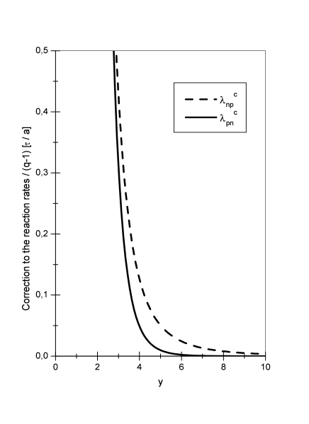
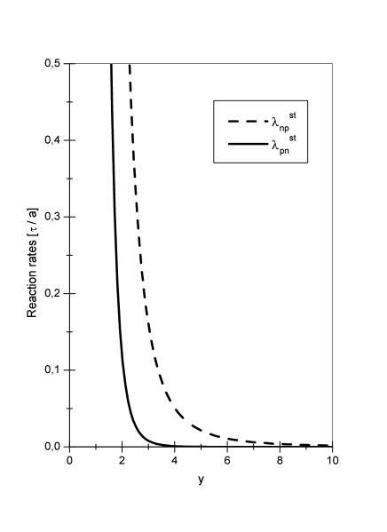
Figure 1: Left: Standard reaction rates λpnst(y)subscriptsuperscript𝜆𝑠𝑡𝑝𝑛𝑦\lambda^{st}_{pn}(y) and λnpst(y)subscriptsuperscript𝜆𝑠𝑡𝑛𝑝𝑦\lambda^{st}_{np}(y). Right: Corrections produced by non-extensive statistics, normalized by (q1)𝑞1(q-1), using the full BNE.

4.2 λpnqsubscriptsuperscript𝜆𝑞𝑝𝑛\lambda^{q}_{pn}

We use Eqs. (29) and (34) to get, within the full BNE,

λpnq(y)=eyλnpq(y)+q12aτy5ey[120y+60y2+12y3+y4].subscriptsuperscript𝜆𝑞𝑝𝑛𝑦superscript𝑒𝑦subscriptsuperscript𝜆𝑞𝑛𝑝𝑦𝑞12𝑎𝜏superscript𝑦5superscript𝑒𝑦delimited-[]120𝑦60superscript𝑦212superscript𝑦3superscript𝑦4\lambda^{q}_{pn}(y)=e^{-y}\lambda^{q}_{np}(y)+\frac{q-1}{2}\frac{a}{\tau y^{5}}e^{-y}\left[120y+60y^{2}+12y^{3}+y^{4}\right]. (36)

It is also immediate to obtain this rate in the BST, i.e.

λpnq(y)=eyλnpq(y).subscriptsuperscript𝜆𝑞𝑝𝑛𝑦superscript𝑒𝑦subscriptsuperscript𝜆𝑞𝑛𝑝𝑦\lambda^{q}_{pn}(y)=e^{-y}\lambda^{q}_{np}(y). (37)

This last equation was used by Torres and Vucetich [3], where the BST was assumed from the beginning.

It is worth noticing that since λpnst(y)subscriptsuperscript𝜆𝑠𝑡𝑝𝑛𝑦\lambda^{st}_{pn}(y) and λnpst(y)subscriptsuperscript𝜆𝑠𝑡𝑛𝑝𝑦\lambda^{st}_{np}(y) have an asymptotic behavior analogous to that of the standard rates, see Fig. 1, also in this case we expect that in the limit of low temperatures (i.e. y𝑦y\rightarrow\infty) the neutron abundance behaves as a constant. That is, for low temperatures, the reaction rates are practically zero and then, processes interchanging neutrons into protons and viceversa are negligible. In this sense, Xq(y)superscript𝑋𝑞𝑦X^{q}(y\rightarrow\infty) stabilizes towards a constant.

5 Evolution of the neutron abundance

The formal solution for the evolution of the neutron abundance is given by Eq. (7). We shall use the variable y=Δm/T𝑦Δ𝑚𝑇y=\Delta m/T, so that

Xq(y)=λpnq(y)Λq(y)0y𝑑yIq(y,y)ddy(λpnq(y)Λq(y)),superscript𝑋𝑞𝑦subscriptsuperscript𝜆𝑞𝑝𝑛𝑦superscriptΛ𝑞𝑦superscriptsubscript0𝑦differential-dsuperscript𝑦superscript𝐼𝑞𝑦superscript𝑦𝑑𝑑superscript𝑦subscriptsuperscript𝜆𝑞𝑝𝑛superscript𝑦superscriptΛ𝑞superscript𝑦X^{q}(y)=\frac{\lambda^{q}_{pn}(y)}{\Lambda^{q}(y)}-\int_{0}^{y}dy^{\prime}I^{q}(y,y^{\prime})\frac{d}{dy^{\prime}}\left(\frac{\lambda^{q}_{pn}(y^{\prime})}{\Lambda^{q}(y^{\prime})}\right), (38)

and the factor I𝐼I becomes

Iq(y,y)=exp(yy𝑑y^(dt^dy^)Λq(y^)).superscript𝐼𝑞𝑦superscript𝑦superscriptsubscriptsuperscript𝑦𝑦differential-d^𝑦𝑑^𝑡𝑑^𝑦superscriptΛ𝑞^𝑦I^{q}(y,y^{\prime})=\exp{\left(-\int_{y^{\prime}}^{y}d\hat{y}\left(\frac{d\hat{t}}{d\hat{y}}\right)\Lambda^{q}(\hat{y})\right)}. (39)

To evaluate the Jacobian dt^/dy^𝑑^𝑡𝑑^𝑦{d\hat{t}}/{d\hat{y}}, we recall that the scale factor, R𝑅R, in a Friedmann-Robertson-Walker metric, goes as R1/Tsimilar-to-or-equals𝑅1𝑇R\simeq 1/T, independently of the statistics [8]. Then, T˙/T=R˙/R˙𝑇𝑇˙𝑅𝑅\dot{T}/T=-\dot{R}/R, and the rhs is given by Einstein equations,

R˙R=(8πG3ρq)1/2.˙𝑅𝑅superscript8𝜋𝐺3subscript𝜌𝑞12\frac{\dot{R}}{R}=\left(\frac{8\pi G}{3}\rho_{q}\right)^{1/2}. (40)

Here, ρqsubscript𝜌𝑞\rho_{q} is the energy density of relativistic species, given in Paper I. When the universe is dominated by e,e+,νsuperscript𝑒superscript𝑒𝜈e^{-},e^{+},\nu and γssuperscript𝛾𝑠\gamma^{\prime}s, and then gb=2subscript𝑔𝑏2g_{b}=2, gf=2+2+2×3=10subscript𝑔𝑓222310g_{f}=2+2+2\times 3=10 and g=bgb+78fgf=43/4𝑔subscript𝑏superscript𝑔𝑏78subscript𝑓superscript𝑔𝑓434g=\sum_{b}g^{b}+\frac{7}{8}\sum_{f}g^{f}=43/4, we obtain

ρq=π230gT4+35.85(q1)T4.subscript𝜌𝑞superscript𝜋230𝑔superscript𝑇435.85𝑞1superscript𝑇4\rho_{q}=\frac{\pi^{2}}{30}gT^{4}+35.85(q-1)T^{4}. (41)

We can now compute dt/dy𝑑𝑡𝑑𝑦dt/dy,

dtdy=dtdTdTdy=1T˙Δmy2.𝑑𝑡𝑑𝑦𝑑𝑡𝑑𝑇𝑑𝑇𝑑𝑦1˙𝑇Δ𝑚superscript𝑦2\frac{dt}{dy}=\frac{dt}{dT}\frac{dT}{dy}=-\frac{1}{\dot{T}}\frac{\Delta m}{y^{2}}. (42)

Since, T˙/T=R˙/R˙𝑇𝑇˙𝑅𝑅\dot{T}/T=-\dot{R}/R,

T˙=T(8πG3ρq)1/2,˙𝑇𝑇superscript8𝜋𝐺3subscript𝜌𝑞12\dot{T}=-T\left(\frac{8\pi G}{3}\rho_{q}\right)^{1/2}, (43)

and to first order in (q1)𝑞1(q-1),

1T˙=1T3(454π3Gg)1/2[115gπ235.85(q1)].1˙𝑇1superscript𝑇3superscript454superscript𝜋3𝐺𝑔12delimited-[]115𝑔superscript𝜋235.85𝑞1\frac{1}{\dot{T}}=-\frac{1}{T^{3}}\left(\frac{45}{4\pi^{3}Gg}\right)^{1/2}\left[1-\frac{15}{g\pi^{2}}35.85(q-1)\right]. (44)

In this sense, we see that

dtdy=τaby[1c(q1)],𝑑𝑡𝑑𝑦𝜏𝑎𝑏𝑦delimited-[]1𝑐𝑞1\frac{dt}{dy}=\frac{\tau}{a}by\left[1-c(q-1)\right], (45)

where b𝑏b and c𝑐c are given

b=(454π3Gg)1/2aτΔm2,c=15gπ235.85.formulae-sequence𝑏superscript454superscript𝜋3𝐺𝑔12𝑎𝜏Δsuperscript𝑚2𝑐15𝑔superscript𝜋235.85b=\left(\frac{45}{4\pi^{3}Gg}\right)^{1/2}\frac{a}{\tau\Delta m^{2}},\;\;\;\;\;\;\;c=\frac{15}{g\pi^{2}}35.85. (46)

Numerical values for these constants can be obtained taking into account that: a=255𝑎255a=255, g=43/4𝑔434g=43/4, Δm=1.29Δ𝑚1.29\Delta m=1.29MeV, τ=887±2𝜏plus-or-minus8872\tau=887\pm 2s [9] and G=mpl2𝐺superscriptsubscript𝑚𝑝𝑙2G=m_{pl}^{-2} and are b=0.25𝑏0.25b=0.25 and c=5.07𝑐5.07c=5.07. This follows the treatment given in Ref. [3].

Using all previous remarks,

Iq(y,y)=exp(Kq(y)Kq(y)),superscript𝐼𝑞𝑦superscript𝑦superscript𝐾𝑞𝑦superscript𝐾𝑞superscript𝑦I^{q}(y,y^{\prime})=\exp{(K^{q}(y)-K^{q}(y^{\prime}))}, (47)

with Kq(y)superscript𝐾𝑞𝑦K^{q}(y) given by

Kq(y)=𝑑y^(dt^dy^)Λq(y^),superscript𝐾𝑞𝑦differential-d^𝑦𝑑^𝑡𝑑^𝑦superscriptΛ𝑞^𝑦K^{q}(y)=-\int d\hat{y}\left(\frac{d\hat{t}}{d\hat{y}}\right)\Lambda^{q}(\hat{y}), (48)

or, equivalently, using Eq. (45),

Kq(y)=τba(1c(q1))𝑑y^y^Λq(y^).superscript𝐾𝑞𝑦𝜏𝑏𝑎1𝑐𝑞1differential-d^𝑦^𝑦superscriptΛ𝑞^𝑦K^{q}(y)=-\frac{\tau b}{a}(1-c(q-1))\int d\hat{y}\hat{y}\Lambda^{q}(\hat{y}). (49)

We then see that the needed steps to solve for the evolution of Xqsuperscript𝑋𝑞X^{q} as a function of y𝑦y are: 1) find the function Kq(y)superscript𝐾𝑞𝑦K^{q}(y) as in Eq. (49), 2) substitute this result in the expression (47) for Iq(y,y)superscript𝐼𝑞𝑦superscript𝑦I^{q}(y,y^{\prime}), and 3) finally solve the integral in (38). The complexity of all functions involved requires a numerical procedure. However, we can do further before going to numerical work, since our aim is to primarily see how the asymptotic value of X𝑋X, Xq(y)superscript𝑋𝑞𝑦X^{q}(y\rightarrow\infty), is affected as a function of the parameter (q1)𝑞1(q-1), and ultimately, how this asymptotic value changes if one assume the full BNE as compared with the approximate BST approach.

6 Standard Balance: BST

In this case, λq(y)/Λq(y)superscript𝜆𝑞𝑦superscriptΛ𝑞𝑦\lambda^{q}(y)/\Lambda^{q}(y) coincides with its standard analogous λst(y)/Λst(y)superscript𝜆𝑠𝑡𝑦superscriptΛ𝑠𝑡𝑦\lambda^{st}(y)/\Lambda^{st}(y). Indeed, by definition, Λq(y)=λpnq(y)+λnpq(y)superscriptΛ𝑞𝑦subscriptsuperscript𝜆𝑞𝑝𝑛𝑦subscriptsuperscript𝜆𝑞𝑛𝑝𝑦\Lambda^{q}(y)=\lambda^{q}_{pn}(y)+\lambda^{q}_{np}(y), and since BST establishes λpnq(y)=eyλnpq(y)subscriptsuperscript𝜆𝑞𝑝𝑛𝑦superscript𝑒𝑦subscriptsuperscript𝜆𝑞𝑛𝑝𝑦\lambda^{q}_{pn}(y)=e^{-y}\lambda^{q}_{np}(y), we obtain λq(y)/Λq(y)=(1+ey)1=λst(y)/Λstsuperscript𝜆𝑞𝑦superscriptΛ𝑞𝑦superscript1superscript𝑒𝑦1superscript𝜆𝑠𝑡𝑦superscriptΛ𝑠𝑡\lambda^{q}(y)/\Lambda^{q}(y)=(1+e^{y})^{-1}=\lambda^{st}(y)/\Lambda^{st}.

We can get Kq(y)superscript𝐾𝑞𝑦K^{q}(y) taking into account that, using Eqs. (35) and (36),

Λq(y)=aτy5(1+ey)[12+6y+y2]+(q1)[180+60y+6y2].superscriptΛ𝑞𝑦𝑎𝜏superscript𝑦51superscript𝑒𝑦delimited-[]126𝑦superscript𝑦2𝑞1delimited-[]18060𝑦6superscript𝑦2\Lambda^{q}(y)=\frac{a}{\tau y^{5}}(1+e^{y})\left[12+6y+y^{2}\right]+(q-1)\left[180+60y+6y^{2}\right]. (50)

Computing the integral in Eq. (49),

Kq(y)=b(1c(q1))[K1(y)+q12K2(y)].superscript𝐾𝑞𝑦𝑏1𝑐𝑞1delimited-[]subscript𝐾1𝑦𝑞12subscript𝐾2𝑦K^{q}(y)=b(1-c(q-1))[K_{1}(y)+\frac{q-1}{2}K_{2}(y)]. (51)

with

K1(y)=[(4y3+3y2+1y)+(4y3+1y2)ey]subscript𝐾1𝑦delimited-[]4superscript𝑦33superscript𝑦21𝑦4superscript𝑦31superscript𝑦2superscript𝑒𝑦K_{1}(y)=\left[\left(\frac{4}{y^{3}}+\frac{3}{y^{2}}+\frac{1}{y}\right)+\left(\frac{4}{y^{3}}+\frac{1}{y^{2}}\right)e^{-y}\right] (52)

and

K2(y)=[(30y3+15y2+3y)+(30y3+3y)ey3Ei(1,y)],subscript𝐾2𝑦delimited-[]30superscript𝑦315superscript𝑦23𝑦30superscript𝑦33𝑦superscript𝑒𝑦3𝐸𝑖1𝑦K_{2}(y)=\left[\left(\frac{30}{y^{3}}+\frac{15}{y^{2}}+\frac{3}{y}\right)+\left(\frac{30}{y^{3}}+\frac{3}{y}\right)e^{-y}-3Ei(1,y)\right], (53)

and where the functions Ei(1,y)𝐸𝑖1𝑦Ei(1,y) are

Ei(1,y)=1eytt𝑑t.𝐸𝑖1𝑦superscriptsubscript1superscript𝑒𝑦𝑡𝑡differential-d𝑡Ei(1,y)=\int_{1}^{\infty}\frac{e^{-yt}}{t}dt. (54)

We recognize in Eq. (51) the standard term Kst(y)=bK1(y)superscript𝐾𝑠𝑡𝑦𝑏subscript𝐾1𝑦K^{st}(y)=bK_{1}(y). The presence of the factor b(1c(q1))𝑏1𝑐𝑞1b(1-c(q-1)) in the Jacobian dt/dy𝑑𝑡𝑑𝑦dt/dy produces the appearance in K2(y)subscript𝐾2𝑦K_{2}(y) of a second order term in (q1)𝑞1(q-1). It is important to note that because this function diverges as y3superscript𝑦3y^{-3} at the origin, it is not a priori obvious that we can retain (as was done in [3]), only the term linear in (q1)𝑞1(q-1). This is a key remark, and we shall come back on this later.

We shall then try to obtain the whole solution, without linearizing any of the functions involving (q1)𝑞1(q-1). Having shown that λq(y)/Λq(y)=(1+ey)1superscript𝜆𝑞𝑦superscriptΛ𝑞𝑦superscript1superscript𝑒𝑦1\lambda^{q}(y)/\Lambda^{q}(y)=(1+e^{y})^{-1}, we can write, using Eq. (38), the asymptotic value Xq()limyXq(y)superscript𝑋𝑞subscript𝑦superscript𝑋𝑞𝑦X^{q}(\infty)\equiv\lim_{y\to\infty}X^{q}(y), as

Xq()=limyeKq(y)0yeKq(y)ey(1+ey)2𝑑y.superscript𝑋𝑞subscript𝑦superscript𝑒superscript𝐾𝑞𝑦superscriptsubscript0𝑦superscript𝑒superscript𝐾𝑞superscript𝑦superscript𝑒superscript𝑦superscript1superscript𝑒superscript𝑦2differential-dsuperscript𝑦X^{q}(\infty)=\lim_{y\to\infty}e^{K^{q}(y)}\int_{0}^{y}e^{-K^{q}(y^{\prime})}\frac{e^{y^{\prime}}}{(1+e^{y^{\prime}})^{2}}dy^{\prime}. (55)

This expression allows for an analytical study. Based on the divergent behavior of Kqsuperscript𝐾𝑞K^{q} at the origin and because of the good behavior of

ddy(λpnq(y)Λq(y))=ey(1+ey)2,𝑑𝑑superscript𝑦subscriptsuperscript𝜆𝑞𝑝𝑛superscript𝑦superscriptΛ𝑞superscript𝑦superscript𝑒superscript𝑦superscript1superscript𝑒superscript𝑦2\frac{d}{dy^{\prime}}\left(\frac{\lambda^{q}_{pn}(y^{\prime})}{\Lambda^{q}(y^{\prime})}\right)=\frac{e^{y^{\prime}}}{(1+e^{y^{\prime}})^{2}}, (56)

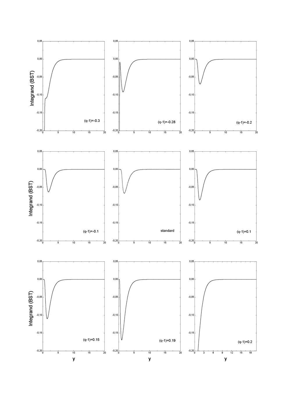
near zero, it is possible to discard a priori, i.e. without having the need to compare with any observation, the range of (q1)𝑞1(q-1)-values such that the non-extensive theory, considered within the BST, looses its sense (i.e. the cases in which the asymptotic values predicted for Xqsuperscript𝑋𝑞X^{q} are out of the interval [0,1/2]). Indeed, in order to avoid problems at the origin in Eq. (55), Kq(y)superscript𝐾𝑞𝑦K^{q}(y) has to be positive when y0𝑦0y\rightarrow 0. Using Eqs. (51), (52) and (53), this condition translates immediately into an allowed interval for (q1)𝑞1(q-1), since

limy0Kq(y)limy0b(1c(q1))[4y3+4y3ey+q12(30y3+30yey)],similar-to-or-equalssubscript𝑦0superscript𝐾𝑞𝑦subscript𝑦0𝑏1𝑐𝑞1delimited-[]4superscript𝑦34superscript𝑦3superscript𝑒𝑦𝑞1230superscript𝑦330𝑦superscript𝑒𝑦\lim_{y\to 0}K^{q}(y)\simeq\lim_{y\to 0}b(1-c(q-1))\left[\frac{4}{y^{3}}+\frac{4}{y^{3}}e^{-y}+\frac{q-1}{2}\left(\frac{30}{y^{3}}+\frac{30}{y}e^{-y}\right)\right], (57)

i.e.

limy0Kq(y)b(1c(q1))[8y3+(q1)30y3].similar-to-or-equalssubscript𝑦0superscript𝐾𝑞𝑦𝑏1𝑐𝑞1delimited-[]8superscript𝑦3𝑞130superscript𝑦3\lim_{y\to 0}K^{q}(y)\simeq b(1-c(q-1))\left[\frac{8}{y^{3}}+(q-1)\frac{30}{y^{3}}\right]. (58)

We see that, to have Kq(y)>0superscript𝐾𝑞𝑦0K^{q}(y)>0, (q1)𝑞1(q-1) must be such that the inequality 8/30<(q1)<1/c830𝑞11𝑐-8/30<(q-1)<1/c is fulfilled. Recalling that c=5.07𝑐5.07c=5.07 we see that values that do not fulfill the condition

0.27<(q1)<0.20.27𝑞10.2\displaystyle-0.27<(q-1)<0.2 (59)

must be automatically discarded. We mention in addition that no matter the sign of Kqsuperscript𝐾𝑞K^{q}, the factor eK(y)superscript𝑒𝐾𝑦e^{K(y)} multiplying the integral in Eq. (55) tends to 1 when y𝑦y\rightarrow\infty.

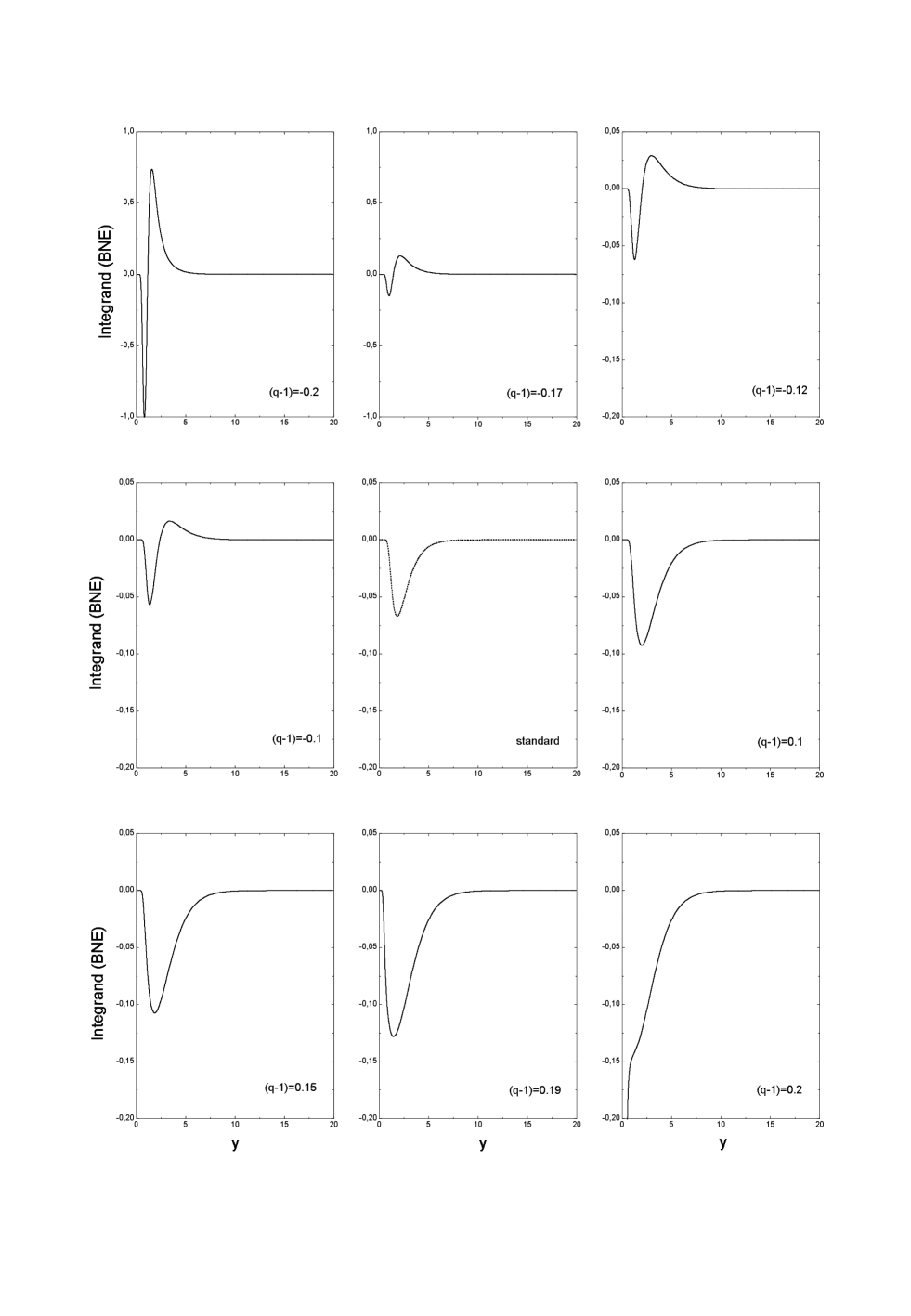
Fig. 2 shows the behavior of the integrand of Eq. (55) for different (q1)𝑞1(q-1)-values. Note the abrupt change of the plots when (q1)𝑞1(q-1) is near the extremes of the range given by Eq. (59). The analytical conclusion is then reinforced by these plots and is completely confirmed when numerical computations are made. These latter show that the integral (55) grows without limit when (q1)𝑞1(q-1) assumes values out of the range given by Eq. (59).
Refer to caption
Figure 2: Behavior of the integrand needed in the computation of Xq()superscript𝑋𝑞X^{q}(\infty) for different values of (q1)𝑞1(q-1) within the BST approach.

We have then showed that there exist a range of (q1)𝑞1(q-1) such that the asymptotic value of Xq()superscript𝑋𝑞X^{q}(\infty) has physical sense. We can now ask if there also exist a range of (q1)[0.27,0.2]𝑞10.270.2(q-1)\in[-0.27,0.2] such that the Xq()superscript𝑋𝑞X^{q}(\infty) obtained to first order in (q1)𝑞1(q-1) is consistent with the whole computation. This would be so if we can prove that the first order result do not differ much from the real result that we have already got.

6.1 First order computation

To compute Xq()superscript𝑋𝑞X^{q}(\infty) to first order in (q1)𝑞1(q-1), we need to write Eq. (55) to first order and neglect quadratic terms in Eq. (51). This gives

Kq(y)=Kst(y)+(q1)Kc(y),superscript𝐾𝑞𝑦superscript𝐾𝑠𝑡𝑦𝑞1superscript𝐾𝑐𝑦K^{q}(y)=K^{st}(y)+(q-1)K^{c}(y), (60)

with

Kst(y)=b[(4y3+3y2+1y)+(4y3+1y2)ey],superscript𝐾𝑠𝑡𝑦𝑏delimited-[]4superscript𝑦33superscript𝑦21𝑦4superscript𝑦31superscript𝑦2superscript𝑒𝑦K^{st}(y)=b\left[\left(\frac{4}{y^{3}}+\frac{3}{y^{2}}+\frac{1}{y}\right)+\left(\frac{4}{y^{3}}+\frac{1}{y^{2}}\right)e^{-y}\right], (61)

and

Kc(y)=b2[(30y3+15y2+3y)+(30y3+3y)ey3Ei(1,y)]cKst.superscript𝐾𝑐𝑦𝑏2delimited-[]30superscript𝑦315superscript𝑦23𝑦30superscript𝑦33𝑦superscript𝑒𝑦3𝐸𝑖1𝑦𝑐superscript𝐾𝑠𝑡K^{c}(y)=\frac{b}{2}\left[\left(\frac{30}{y^{3}}+\frac{15}{y^{2}}+\frac{3}{y}\right)+\left(\frac{30}{y^{3}}+\frac{3}{y}\right)e^{-y}-3Ei(1,y)\right]-cK^{st}. (62)

We write eKqsuperscript𝑒superscript𝐾𝑞e^{K^{q}} to first order as

eKq=eKste(q1)KceKst[1+(q1)Kc].superscript𝑒superscript𝐾𝑞superscript𝑒superscript𝐾𝑠𝑡superscript𝑒𝑞1superscript𝐾𝑐similar-to-or-equalssuperscript𝑒superscript𝐾𝑠𝑡delimited-[]1𝑞1superscript𝐾𝑐e^{K^{q}}=e^{K^{st}}e^{(q-1)K^{c}}\simeq e^{K^{st}}[1+(q-1)K^{c}]. (63)

Substituting this expansion into (55) and retaining only the linear term we get

Xq()=Xst()+(q1)Xc(),superscript𝑋𝑞superscript𝑋𝑠𝑡𝑞1superscript𝑋𝑐X^{q}(\infty)=X^{st}(\infty)+(q-1)X^{c}(\infty), (64)

with

Xst()=limyeKst(y)0yeKst(y)ey(1+ey)2𝑑y,superscript𝑋𝑠𝑡subscript𝑦superscript𝑒superscript𝐾𝑠𝑡𝑦superscriptsubscript0𝑦superscript𝑒superscript𝐾𝑠𝑡superscript𝑦superscript𝑒superscript𝑦superscript1superscript𝑒superscript𝑦2differential-dsuperscript𝑦X^{st}(\infty)=\lim_{y\to\infty}e^{K^{st}(y)}\int_{0}^{y}e^{-K^{st}(y^{\prime})}\frac{e^{y^{\prime}}}{(1+e^{y^{\prime}})^{2}}dy^{\prime}, (65)

and

Xc()=limyeKst(y)0yeKst(y)[Kc(y)Kc(y)]ey(1+ey)2𝑑y.superscript𝑋𝑐subscript𝑦superscript𝑒superscript𝐾𝑠𝑡𝑦superscriptsubscript0𝑦superscript𝑒subscript𝐾𝑠𝑡superscript𝑦delimited-[]superscript𝐾𝑐𝑦superscript𝐾𝑐superscript𝑦superscript𝑒superscript𝑦superscript1superscript𝑒superscript𝑦2differential-dsuperscript𝑦X^{c}(\infty)=\lim_{y\to\infty}e^{K^{st}(y)}\int_{0}^{y}e^{-K_{st}(y^{\prime})}[K^{c}(y)-K^{c}(y^{\prime})]\frac{e^{y^{\prime}}}{(1+e^{y^{\prime}})^{2}}dy^{\prime}. (66)

This integrals can be computed numerically, and the result is

Xq()=0.15+(q1)0.18superscript𝑋𝑞0.15𝑞10.18X^{q}(\infty)=0.15+(q-1)0.18 (67)

where the value Xst()=0.15superscript𝑋𝑠𝑡0.15X^{st}(\infty)=0.15 is the standard one.

Refer to caption
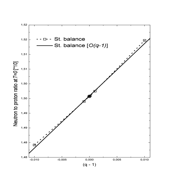
Figure 3: Comparison between Xq()superscript𝑋𝑞X^{q}(\infty) as a function of (q1)𝑞1(q-1), to first order, and using the full numerical solution, both obtained within the BST approach.

Fig. 3 shows the linear dependence of Eq. (67), together with the full solution given by Eq. (55). Although within the framework of the asymptotic approach to quantum distribution functions, an analogous equation to (67) was presented already by some of us [3], we have now shown, for the first time, what is behind that approach, what sustains it, and the range of its validity.

7 Non-extensive balance: BNE

In this section we shall solve Eq. (38) without approximations. That is, we shall take for λpnqsubscriptsuperscript𝜆𝑞𝑝𝑛\lambda^{q}_{pn} and λnpqsubscriptsuperscript𝜆𝑞𝑛𝑝\lambda^{q}_{np}, the expressions given by (35) and (36), respectively. Our aim will be to quantify the amount of the deviation that it is produced when the BST, instead of the full BNE, is considered.

By definition, Λq(y)=λpnq(y)+λnpq(y)superscriptΛ𝑞𝑦superscriptsubscript𝜆𝑝𝑛𝑞𝑦superscriptsubscript𝜆𝑛𝑝𝑞𝑦\Lambda^{q}(y)=\lambda_{pn}^{q}(y)+\lambda_{np}^{q}(y), adding (35) and (36) we see that Λq(y)superscriptΛ𝑞𝑦\Lambda^{q}(y) is given by the sum of two terms

Λst(y)=aτy5(12+6y+y2)[1+ey],superscriptΛ𝑠𝑡𝑦𝑎𝜏superscript𝑦5126𝑦superscript𝑦2delimited-[]1superscript𝑒𝑦\Lambda^{st}(y)=\frac{a}{\tau y^{5}}(12+6y+y^{2})\left[1+e^{-y}\right], (68)
Λc(y)=12aτy5[90[1+ey]+30y[1+5ey]+y2[1+21ey]+12y3+y4].superscriptΛ𝑐𝑦12𝑎𝜏superscript𝑦5delimited-[]90delimited-[]1superscript𝑒𝑦30𝑦delimited-[]15superscript𝑒𝑦superscript𝑦2delimited-[]121superscript𝑒𝑦12superscript𝑦3superscript𝑦4\Lambda^{c}(y)=\frac{1}{2}\frac{a}{\tau y^{5}}\left[90\left[1+e^{-y}\right]+30y\left[1+5e^{-y}\right]+y^{2}\left[1+21e^{-y}\right]+12y^{3}+y^{4}\right]. (69)

Because of the linearity of the integral operator, the same happens to Kq(y)superscript𝐾𝑞𝑦K^{q}(y) in Eq. (49). Using the previous expressions, we get

Kq(y)=b(1c(q1))[K^1(y)+q12K^2(y)].superscript𝐾𝑞𝑦𝑏1𝑐𝑞1delimited-[]subscript^𝐾1𝑦𝑞12subscript^𝐾2𝑦K^{q}(y)=b(1-c(q-1))[\hat{K}_{1}(y)+\frac{q-1}{2}\hat{K}_{2}(y)]. (70)

with

K^1(y)=[(4y3+3y2+1y)+(4y3+1y2)ey]subscript^𝐾1𝑦delimited-[]4superscript𝑦33superscript𝑦21𝑦4superscript𝑦31superscript𝑦2superscript𝑒𝑦\hat{K}_{1}(y)=\left[\left(\frac{4}{y^{3}}+\frac{3}{y^{2}}+\frac{1}{y}\right)+\left(\frac{4}{y^{3}}+\frac{1}{y^{2}}\right)e^{-y}\right] (71)

and

K^2(y)=[(30y3+15y2+3y)+(30y3+60y2+3y)eyy12lny3Ei(1,y)]subscript^𝐾2𝑦delimited-[]30superscript𝑦315superscript𝑦23𝑦30superscript𝑦360superscript𝑦23𝑦superscript𝑒𝑦𝑦12𝑦3𝐸𝑖1𝑦\hat{K}_{2}(y)=\left[\left(\frac{30}{y^{3}}+\frac{15}{y^{2}}+\frac{3}{y}\right)+\left(\frac{30}{y^{3}}+\frac{60}{y^{2}}+\frac{3}{y}\right)e^{-y}-y-12\ln y-3Ei(1,y)\right] (72)

where Ei(1,y)𝐸𝑖1𝑦Ei(1,y) were given in (54). As before, we do recognize the standard term Kst(y)=bK^1(y)superscript𝐾𝑠𝑡𝑦𝑏subscript^𝐾1𝑦K^{st}(y)=b\hat{K}_{1}(y). Also here, within the BNE, it happens that

limyλpnq(y)Λq(y)=0.subscript𝑦subscriptsuperscript𝜆𝑞𝑝𝑛𝑦superscriptΛ𝑞𝑦0\lim_{y\to\infty}\frac{\lambda^{q}_{pn}(y)}{\Lambda^{q}(y)}=0. (73)

Indeed, since within the BNE, in the limit y𝑦y\rightarrow\infty we have λpnq(y)y3proportional-tosubscriptsuperscript𝜆𝑞𝑝𝑛𝑦superscript𝑦3\lambda^{q}_{pn}(y)\propto y^{-3} and λnpq(y)y1eyproportional-tosubscriptsuperscript𝜆𝑞𝑛𝑝𝑦superscript𝑦1superscript𝑒𝑦\lambda^{q}_{np}(y)\propto y^{-1}e^{-y}, we obtain

limyλpnq(y)Λq(y)=limy11+λpnq(y)/Λq(y)=limy11+ey=0.subscript𝑦subscriptsuperscript𝜆𝑞𝑝𝑛𝑦superscriptΛ𝑞𝑦subscript𝑦11subscriptsuperscript𝜆𝑞𝑝𝑛𝑦superscriptΛ𝑞𝑦subscript𝑦11superscript𝑒𝑦0\lim_{y\to\infty}\frac{\lambda^{q}_{pn}(y)}{\Lambda^{q}(y)}=\lim_{y\to\infty}\frac{1}{1+\lambda^{q}_{pn}(y)/\Lambda^{q}(y)}=\lim_{y\to\infty}\frac{1}{1+e^{y}}=0. (74)

We then obtain an analogous to Eq. (55)

Xq()=limyeKq(y)0yeKq(y)ddy(λnpq(y)λpnq(y))𝑑y.superscript𝑋𝑞subscript𝑦superscript𝑒superscript𝐾𝑞𝑦superscriptsubscript0𝑦superscript𝑒superscript𝐾𝑞superscript𝑦𝑑𝑑superscript𝑦subscriptsuperscript𝜆𝑞𝑛𝑝𝑦subscriptsuperscript𝜆𝑞𝑝𝑛𝑦differential-dsuperscript𝑦X^{q}(\infty)=-\lim_{y\to\infty}e^{K^{q}(y)}\int_{0}^{y}e^{-K^{q}(y^{\prime})}\frac{d}{dy^{\prime}}\left(\frac{\lambda^{q}_{np}(y)}{\lambda^{q}_{pn}(y)}\right)dy^{\prime}. (75)

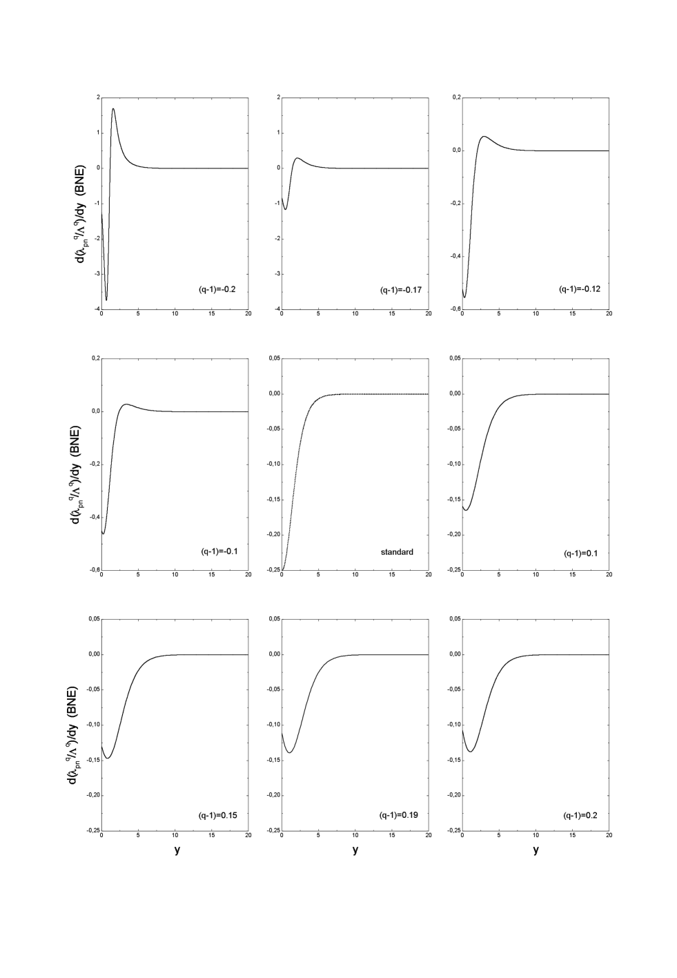
It is important to note that Kq(y)superscript𝐾𝑞𝑦K^{q}(y) diverges as y3superscript𝑦3y^{-3} at the origin, and as y𝑦-y at infinity. Then, first order developments will not do. The complex dependencies of the integrand of Eq. (38) with (q1)𝑞1(q-1) makes much harder to a priori analyze the validity range, as done within the BST. We can, however, make a detailed analysis of the behavior of the derivative of the function λpnq(y)/Λq(y)subscriptsuperscript𝜆𝑞𝑝𝑛𝑦superscriptΛ𝑞𝑦\lambda^{q}_{pn}(y)/\Lambda^{q}(y) and of the integrand of Eq. (38), for different (q1)𝑞1(q-1)-values. We show this in Figs. 4 and 5.
Refer to caption
Figure 4: Behavior of the derivative of λpnq(y)/Λq(y)subscriptsuperscript𝜆𝑞𝑝𝑛𝑦superscriptΛ𝑞𝑦\lambda^{q}_{pn}(y)/\Lambda^{q}(y) for different (q1)𝑞1(q-1)-values within the BNE.
Refer to caption
Figure 5: Behavior of the integrand involved in the computation of Xq()superscript𝑋𝑞X^{q}(\infty) for different (q1)𝑞1(q-1)-values, within the BNE.

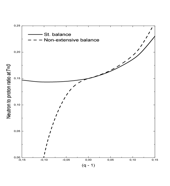
From the analysis of these figures we see that the BST and the BNE differ in a fundamental way, which translates into the value of Xq()superscript𝑋𝑞X^{q}(\infty). Within the BNE, and because of the behavior of the derivative of the function λpnq(y)/Λq(y)subscriptsuperscript𝜆𝑞𝑝𝑛𝑦superscriptΛ𝑞𝑦\lambda^{q}_{pn}(y)/\Lambda^{q}(y) for negative values of (q1)𝑞1(q-1), it is not guaranteed that the integrand in Eq. (38) is negative. For (q1)<0.1𝑞10.1(q-1)<-0.1 the integral of (38) is positive (i.e. Xq()<0superscript𝑋𝑞0X^{q}(\infty)<0), and this discards values of q𝑞q such that (q1)<0.1𝑞10.1(q-1)<-0.1. On the other hand, looking at Fig. 4 for positive values of (q1)𝑞1(q-1), we see that the upper bound is between 0.19 and 0.2, in this case similarly to the BST. Then, for the BNE, the values for which the theory has physical sense a priori of any experimental comparison are

0.1<(q1)<0.2.0.1𝑞10.2-0.1<(q-1)<0.2. (76)

The BNE is more restrictive than the BST. Out of this range, the physical sense of the description is lost.

8 Comparing both approaches, and bounding the value of q𝑞q

We now compare the results obtained in Sections 6 and 7. Fig. 6 shows Xq()superscript𝑋𝑞X^{q}(\infty) for different values of (q1)𝑞1(q-1), both in the full BNE as well as in the BST approximation. Differences are notable, and they grow with increasing values of |q1|𝑞1|q-1|, as it tends to its limiting values. Table 1 gives the explicit values of Xq()superscript𝑋𝑞X^{q}(\infty) obtained using a numerical integration scheme for the BST and for the full BNE, and the analytical results of the first order approximation for the BST. For values of (q1)𝑞1(q-1) near 0, the BST numerical computation is perfectly described by the linear approximation.
Refer to caption
Figure 6: Xq()superscript𝑋𝑞X^{q}(\infty) as a function of (q1)𝑞1(q-1), both for the full BNE and the BST.
Table 1: Comparison of Xq()superscript𝑋𝑞X^{q}(\infty)-values as a function of (q1)𝑞1(q-1) for the different approaches.
(q1)𝑞1(q-1) Xqsuperscript𝑋𝑞X^{q} (BST) Xqsuperscript𝑋𝑞X^{q} (BST) Xqsuperscript𝑋𝑞X^{q} (BNE)
(O𝑂O (q1)𝑞1(q-1))
-0.150 0.1472 0.1230 -0.6571
-0.120 0.1441 0.1284 -0.1061
-0.100 0.1431 0.1320 0.0261
-0.050 0.1440 0.1410 0.1299
-0.010 0.1484 0.1482 0.1476
-0.001 0.1499 0.1498 0.1498
0.0 0.1500 0.1500 0.1500
0.001 0.1502 0.1502 0.1503
0.010 0.1520 0.1518 0.1523
0.050 0.1625 0.1590 0.1635
0.100 0.1851 0.1680 0.1915
0.120 0.1991 0.1716 0.2109
0.150 0.2303 0.1770 0.2561

The deviation from the standard case is greater for the BNE than for the BST, for equal values of (q1)𝑞1(q-1), i.e. the BST underestimates the effect of non-extensivity. This can be seen directly from Fig. 6, or equivalently from Table 2, where we show the coefficients of the linear fit of Xq()superscript𝑋𝑞X^{q}(\infty) near 0, both for the full BNE and the BST. In the sake of completeness, we also show the first order result for the BST (this is not a fit, but comes directly from the analytical computations shown before).

Table 2: Coefficients of the linear fits of Xq()superscript𝑋𝑞X^{q}(\infty) near (q1)=0𝑞10(q-1)=0 for the full BNE, the BST approximation, and for the first order computation of the BST.
Case Xstsuperscript𝑋𝑠𝑡X^{st} Xcsuperscript𝑋𝑐X^{c}
BST Approximation 0.15 0.18
BST O(q1)𝑂𝑞1O(q-1) 0.15 0.18
BNE Full 0.15 0.23

Until now, we have discussed the physical viability of the statistical description, establishing a range of a priori discarded values of (q1)𝑞1(q-1) both for the full BNE case, the real situation, and for the BST approximation. These values are those for which Xq()superscript𝑋𝑞X^{q}(\infty) is <0absent0<0 or >0.5absent0.5>0.5. This can be done before than the comparison with any given observational data or experiment. Recall that X()𝑋X(\infty) is the neutron to proton ratio, for which clearly, a negative value has no sense. In addition, X()>0.5𝑋0.5X(\infty)>0.5 is in conflict with the reaction rates dependence with temperature, since X=0.5𝑋0.5X=0.5 is the initial condition for the kinetic equation (1) when T𝑇T\rightarrow\infty (i.e. y0𝑦0y\rightarrow 0). Within the range of physical viability we now look for consistency with observations. This will further restrict the range of admitted values of (q1)𝑞1(q-1). To obtain a direct bound upon (q1)𝑞1(q-1) using the primordial abundance of 4He it is necessary to study in detail the free decay of neutrons, happening between the moment of freezing out of the weak interactions (tsimilar-to-or-equals𝑡absentt\simeq 1 s) and the moment in which the temperature of the universe is similar to the binding energy of D (tsimilar-to-or-equals𝑡absentt\simeq 3 minutes). We shall provide, for the first time in a non-extensive setting, a detailed account of this in the following section, but nevertheless, let us give here some preliminary considerations in the sense of Ref. [2].

Including the effects of the neutron decay in the equation for the evolution of Xq(t)superscript𝑋𝑞𝑡X^{q}(t) we have,

Xq(t)=exp(t/τ)X¯q(t),superscript𝑋𝑞𝑡𝑡𝜏superscript¯𝑋𝑞𝑡X^{q}(t)=\exp(-t/\tau)\bar{X}^{q}(t), (77)

where X¯qsuperscript¯𝑋𝑞\bar{X}^{q} is the already obtained ratio and τ𝜏\tau is the neutron mean life. In the capture time, t=tc𝑡subscript𝑡𝑐t=t_{c}, when the temperature is below the D binding energy (2.23 MeV), neutrons are captured into D. Then, almost all neutrons present at t=tc𝑡subscript𝑡𝑐t=t_{c} are converted into 4He. Substituting the value of tcsubscript𝑡𝑐t_{c} into Eq. (77) and using the value of X¯q()superscript¯𝑋𝑞\bar{X}^{q}(\infty) previously found, we shall obtain half of the mass fraction of all 4He primordially produced. For the time being, we shall adopt the standard value for exp(tc/τ)subscript𝑡𝑐𝜏\exp(t_{c}/\tau), which is 0.8similar-to-or-equalsabsent0.8\simeq 0.8 [6]. With this we obtain,

Ypqsubscriptsuperscript𝑌𝑞𝑝\displaystyle Y^{q}_{p} \displaystyle\equiv 2X4qetc/τ2X¯q()similar-to-or-equals2superscriptsubscript𝑋4𝑞superscript𝑒subscript𝑡𝑐𝜏2superscript¯𝑋𝑞\displaystyle 2X_{4}^{q}\simeq e^{-t_{c}/\tau}2\bar{X}^{q}(\infty) (78)
=\displaystyle= 0.8×2×[0.15+(q1)0.23]0.82delimited-[]0.15𝑞10.23\displaystyle 0.8\times 2\times[0.15+(q-1)0.23]
=\displaystyle= 0.24+(q1)0.37.0.24𝑞10.37\displaystyle 0.24+(q-1)0.37.

There is no absolute consensus about the observational value of 4He. The two greatest compilations give [10],

Yp=0.244±0.004andYp=0.234±0.004.formulae-sequencesubscript𝑌𝑝plus-or-minus0.2440.004andsubscript𝑌𝑝plus-or-minus0.2340.004Y_{p}=0.244\pm 0.004\qquad\textrm{and}\qquad Y_{p}=0.234\pm 0.004. (79)

To consider a typical case, we average over the two mean values and twice the error bar,

Yp=0.239±0.008.subscript𝑌𝑝plus-or-minus0.2390.008Y_{p}=0.239\pm 0.008. (80)

If at the same time we neglect the difference between the standard theoretical and the observational values, which is given by 0.001, in order to obtain a first bound, we can get, using Eq. (78) and asking for |q1|0.37<0.008𝑞10.370.008|q-1|0.37<0.008,

|q1|<0.021.𝑞10.021|q-1|<0.021. (81)

Within the most complete treatment of the principle of detailed balance (BNE), which accounts for the more in depth analytical study on the influence of a slight non-extensivity in primordial nucleosynthesis, the value of q𝑞q could differ from 1 at the level of a few percent and still be in agreement with current constraints. See below for a more detailed treatment.

9 The capture time

The aim of this section is to show how the capture time tcsubscript𝑡𝑐t_{c} is modified in the non-extensive framework. Recalling that at early times R˙/R=(8πρq/3mpl)2˙𝑅𝑅superscript8𝜋subscript𝜌𝑞3subscript𝑚𝑝𝑙2\dot{R}/R=(8\pi\rho_{q}/3m_{pl})^{2} and R(t)Tν(t)=constant𝑅𝑡subscript𝑇𝜈𝑡𝑐𝑜𝑛𝑠𝑡𝑎𝑛𝑡R(t)T_{\nu}(t)=constant after the e+esuperscript𝑒superscript𝑒e^{+}e^{-} annihilation, it is straightforward to write

t=(38πG)1/2Tνρq1/2dTνTν+t0,𝑡superscript38𝜋𝐺12superscriptsubscriptsubscript𝑇𝜈superscriptsubscript𝜌𝑞12𝑑subscriptsuperscript𝑇𝜈subscriptsuperscript𝑇𝜈subscript𝑡0t=\left(\frac{3}{8\pi G}\right)^{1/2}\int_{T_{\nu}}^{\infty}\rho_{q}^{-1/2}\frac{dT^{\prime}_{\nu}}{T^{\prime}_{\nu}}+t_{0}, (82)

where t0subscript𝑡0t_{0} is a constant whose standard value is of the order 2 seconds, see [6]. In Paper I, it was shown that the energy density could be written as ρR=(π2/30)gqT4subscript𝜌𝑅superscript𝜋230superscriptsubscript𝑔𝑞superscript𝑇4\rho_{R}=(\pi^{2}/30)g_{*}^{q}T^{4}. Taking also into account that the photon and neutrino temperatures are related by Tγ=(11/4)1/3[1+0.109(q1)]Tνsubscript𝑇𝛾superscript11413delimited-[]10.109𝑞1subscript𝑇𝜈T_{\gamma}=(11/4)^{1/3}[1+0.109(q-1)]T_{\nu}, we can solve the definite integral to obtain:

t=(4516π3geff)1/2(114)2/3mplTγ2[15.06(q1)]+t0,𝑡superscript4516superscript𝜋3subscript𝑔𝑒𝑓𝑓12superscript11423subscript𝑚𝑝𝑙subscriptsuperscript𝑇2𝛾delimited-[]15.06𝑞1subscript𝑡0t=\left(\frac{45}{16\pi^{3}g_{eff}}\right)^{1/2}\left(\frac{11}{4}\right)^{2/3}\frac{m_{pl}}{T^{2}_{\gamma}}[1-5.06(q-1)]+t_{0}, (83)

where geff=2(11/4)4/3+21/412.95subscript𝑔𝑒𝑓𝑓2superscript11443214similar-to-or-equals12.95g_{eff}=2(11/4)^{4/3}+21/4\simeq 12.95.

In equilibrium, neutrons, protons and deuterons behave as free non-relativistic gases, with number densities given by

nqi=gi(miTγ2π)3/2e(miμi)/Tγ×[1+q12(154+3miμiTγ+(miμiTγ)2)].superscriptsubscript𝑛𝑞𝑖subscript𝑔𝑖superscriptsubscript𝑚𝑖subscript𝑇𝛾2𝜋32superscript𝑒subscript𝑚𝑖subscript𝜇𝑖subscript𝑇𝛾delimited-[]1𝑞121543subscript𝑚𝑖subscript𝜇𝑖subscript𝑇𝛾superscriptsubscript𝑚𝑖subscript𝜇𝑖subscript𝑇𝛾2n_{q}^{i}=g_{i}\left(\frac{m_{i}T_{\gamma}}{2\pi}\right)^{3/2}e^{-(m_{i}-\mu_{i})/T_{\gamma}}\times\left[1+\frac{q-1}{2}\left(\frac{15}{4}+3\frac{m_{i}-\mu_{i}}{T_{\gamma}}+\left(\frac{m_{i}-\mu_{i}}{T_{\gamma}}\right)^{2}\right)\right]. (84)

Here, the subscript i𝑖i stands for n,p𝑛𝑝n,p and D𝐷D, for neutrons, protons and deuterons respectively, gn=gp=2,gD=3formulae-sequencesubscript𝑔𝑛subscript𝑔𝑝2subscript𝑔𝐷3g_{n}=g_{p}=2,g_{D}=3 and μi,misubscript𝜇𝑖subscript𝑚𝑖\mu_{i},m_{i} are the chemical potentials and masses of the particles. At early times, these gases are in chemical equilibrium, so that μD=μn+μpsubscript𝜇𝐷subscript𝜇𝑛subscript𝜇𝑝\mu_{D}=\mu_{n}+\mu_{p}. Therefore,

nqnnqpnqD=gngpgD(mnmpmD)3/2(Tγ2π)3/2eϵD/Tγ[u¯((mnμn)/T)u¯((mpμp)/T)u¯((mDμD)/T)],superscriptsubscript𝑛𝑞𝑛superscriptsubscript𝑛𝑞𝑝superscriptsubscript𝑛𝑞𝐷subscript𝑔𝑛subscript𝑔𝑝subscript𝑔𝐷superscriptsubscript𝑚𝑛subscript𝑚𝑝subscript𝑚𝐷32superscriptsubscript𝑇𝛾2𝜋32superscript𝑒subscriptitalic-ϵ𝐷subscript𝑇𝛾delimited-[]¯𝑢subscript𝑚𝑛subscript𝜇𝑛𝑇¯𝑢subscript𝑚𝑝subscript𝜇𝑝𝑇¯𝑢subscript𝑚𝐷subscript𝜇𝐷𝑇\frac{n_{q}^{n}n_{q}^{p}}{n_{q}^{D}}=\frac{g_{n}g_{p}}{g_{D}}\left(\frac{m_{n}m_{p}}{m_{D}}\right)^{3/2}\left(\frac{T_{\gamma}}{2\pi}\right)^{3/2}e^{-\epsilon_{D}/T_{\gamma}}\left[\frac{\bar{u}((m_{n}-\mu_{n})/T)\bar{u}((m_{p}-\mu_{p})/T)}{\bar{u}((m_{D}-\mu_{D})/T)}\right], (85)

with ϵD=mn+mpmDsubscriptitalic-ϵ𝐷subscript𝑚𝑛subscript𝑚𝑝subscript𝑚𝐷\epsilon_{D}=m_{n}+m_{p}-m_{D}, and where we have made use of the definition,

u¯((miμi)/T)1+q12(154+3miμiT+(miμiT)2).¯𝑢subscript𝑚𝑖subscript𝜇𝑖𝑇1𝑞121543subscript𝑚𝑖subscript𝜇𝑖𝑇superscriptsubscript𝑚𝑖subscript𝜇𝑖𝑇2\bar{u}((m_{i}-\mu_{i})/T)\equiv 1+\frac{q-1}{2}\left(\frac{15}{4}+3\frac{m_{i}-\mu_{i}}{T}+\left(\frac{m_{i}-\mu_{i}}{T}\right)^{2}\right). (86)

Equation (85) is the generalized Saha equation that describes the deuterium formation (see Paper I for a general derivation). Helium appearance is inhibited by the “Deuteron bottleneck”, represented by the reactions:

n+p𝑛𝑝\displaystyle n+p \displaystyle\rightarrow D+γ,D𝛾\displaystyle\rm{D}+\gamma, (87)
D+DDD\displaystyle\rm{D}+\rm{D} \displaystyle\rightarrow T+p,Tp\displaystyle\rm{T}+p, (88)
D+TDT\displaystyle\rm{D}+\rm{T} \displaystyle\rightarrow He4+n.superscriptHe4n{}^{4}\!\rm{He}+n. (89)

Eq. (85) can be given in terms of the normalized abundance fractions Xqi=nqi/nqBsuperscriptsubscript𝑋𝑞𝑖superscriptsubscript𝑛𝑞𝑖superscriptsubscript𝑛𝑞𝐵X_{q}^{i}=n_{q}^{i}/n_{q}^{B}. To this purpose we introduce the baryon to photon ratio ηq=nqB/nqγsubscript𝜂𝑞superscriptsubscript𝑛𝑞𝐵superscriptsubscript𝑛𝑞𝛾\eta_{q}=n_{q}^{B}/n_{q}^{\gamma} and recall that nqγ=[2ζ(3)+3!ζ(4)(q1)](Tγ3/π2)superscriptsubscript𝑛𝑞𝛾delimited-[]2𝜁33𝜁4𝑞1subscriptsuperscript𝑇3𝛾superscript𝜋2n_{q}^{\gamma}=[2\zeta(3)+3!\zeta(4)(q-1)](T^{3}_{\gamma}/\pi^{2}). We get for the quantity Gnpq=XqnXqp/XqDsubscriptsuperscript𝐺𝑞𝑛𝑝superscriptsubscript𝑋𝑞𝑛superscriptsubscript𝑋𝑞𝑝superscriptsubscript𝑋𝑞𝐷G^{q}_{np}=X_{q}^{n}X_{q}^{p}/X_{q}^{D}, to first order in (q1)𝑞1(q-1), the following result

Gnpq=π1/2ζ(3)23ηq(mpmn2mDTγ)3/2eϵD/Tγ[1+q12(un+upuD)].subscriptsuperscript𝐺𝑞𝑛𝑝superscript𝜋12𝜁323subscript𝜂𝑞superscriptsubscript𝑚𝑝subscript𝑚𝑛2subscript𝑚𝐷𝑇𝛾32superscript𝑒subscriptitalic-ϵ𝐷subscript𝑇𝛾delimited-[]1𝑞12subscript𝑢𝑛subscript𝑢𝑝subscript𝑢𝐷G^{q}_{np}=\frac{\pi^{1/2}}{\zeta(3)}\frac{2}{3\eta_{q}}\left(\frac{m_{p}m_{n}}{2m_{D}T\gamma}\right)^{3/2}e^{-\epsilon_{D}/T_{\gamma}}\left[1+\frac{q-1}{2}(u_{n}+u_{p}-u_{D})\right]. (90)

Here, as in Paper I, ui=15/4+3(miμi)/T+((miμi)/T)2subscript𝑢𝑖1543subscript𝑚𝑖subscript𝜇𝑖𝑇superscriptsubscript𝑚𝑖subscript𝜇𝑖𝑇2u_{i}=15/4+3(m_{i}-\mu_{i})/T+((m_{i}-\mu_{i})/T)^{2}. As in the standard case analyzed in Ref. [6], to determine the neutron capture time tcsubscript𝑡𝑐t_{c} we need to examine the sequence of reactions (87-89). It is convenient to do so in terms of an scaled temperature z=ϵD/Tγ𝑧subscriptitalic-ϵ𝐷subscript𝑇𝛾z=\epsilon_{D}/T_{\gamma}, so that they involve rate parameters of the form

Rq=dtdzσvTnqB,superscript𝑅𝑞𝑑𝑡𝑑𝑧subscriptdelimited-⟨⟩𝜎𝑣𝑇superscriptsubscript𝑛𝑞𝐵R^{q}=\frac{dt}{dz}\langle\sigma v\rangle_{T}n_{q}^{B}, (91)

where σvTsubscriptdelimited-⟨⟩𝜎𝑣𝑇\langle\sigma v\rangle_{T} denotes the thermal average of the relevant cross section times the relative velocity [6]. Using Eq. (83) and writing the baryon number density in terms of the baryon to photon number density ratio, ηqsubscript𝜂𝑞\eta_{q}, we get

Rq=ηqz2(45π7geff)1/2(114)2/3ζ(3)ϵDmplσvT[1+0.34(q1)].superscript𝑅𝑞subscript𝜂𝑞superscript𝑧2superscript45superscript𝜋7subscript𝑔𝑒𝑓𝑓12superscript11423𝜁3subscriptitalic-ϵ𝐷subscript𝑚𝑝𝑙subscriptdelimited-⟨⟩𝜎𝑣𝑇delimited-[]10.34𝑞1R^{q}=\frac{\eta_{q}}{z^{2}}\left(\frac{45}{\pi^{7}g_{eff}}\right)^{1/2}\left(\frac{11}{4}\right)^{2/3}\zeta(3)\epsilon_{D}m_{pl}\langle\sigma v\rangle_{T}[1+0.34(q-1)]. (92)

Taking η0=3.57×10¹⁰subscript𝜂03.57superscript1010\eta_{0}=3.57\times 10^{10} [9] as a nominal value for ηqsubscript𝜂𝑞\eta_{q} and considering σnpvT=4.6×10²⁰subscriptdelimited-⟨⟩subscript𝜎𝑛𝑝𝑣𝑇4.6superscript1020\langle\sigma_{np}v\rangle_{T}=4.6\times 10^{-20} [11] we obtain

Rnpq=3.63(29z2)2ηqη0[1+0.34(q1)].subscriptsuperscript𝑅𝑞𝑛𝑝3.63superscript29superscript𝑧22subscript𝜂𝑞subscript𝜂0delimited-[]10.34𝑞1R^{q}_{np}=3.63\left(\frac{29}{z^{2}}\right)^{2}\frac{\eta_{q}}{\eta_{0}}[1+0.34(q-1)]. (93)

Neutron and proton populations are mainly determined by the kinetic equations

dXqndz=Rnpq[XqnXqpGnpqXqD],dXqpdz=Rnpq[XqnXqpGnpqXqD].formulae-sequence𝑑superscriptsubscript𝑋𝑞𝑛𝑑𝑧subscriptsuperscript𝑅𝑞𝑛𝑝delimited-[]superscriptsubscript𝑋𝑞𝑛superscriptsubscript𝑋𝑞𝑝subscriptsuperscript𝐺𝑞𝑛𝑝superscriptsubscript𝑋𝑞𝐷𝑑superscriptsubscript𝑋𝑞𝑝𝑑𝑧subscriptsuperscript𝑅𝑞𝑛𝑝delimited-[]superscriptsubscript𝑋𝑞𝑛superscriptsubscript𝑋𝑞𝑝subscriptsuperscript𝐺𝑞𝑛𝑝superscriptsubscript𝑋𝑞𝐷\frac{dX_{q}^{n}}{dz}=-R^{q}_{np}[X_{q}^{n}X_{q}^{p}-G^{q}_{np}X_{q}^{D}],\hskip 65.44142pt\frac{dX_{q}^{p}}{dz}=-R^{q}_{np}[X_{q}^{n}X_{q}^{p}-G^{q}_{np}X_{q}^{D}]. (94)

As in the usual case, if the neutron population is not depleted by other reactions such as Eqs. (88-89), protons, neutrons and deuterons are kept in equilibrium, relationships Xpq+Xnq+2XDq=1subscriptsuperscript𝑋𝑞𝑝subscriptsuperscript𝑋𝑞𝑛2subscriptsuperscript𝑋𝑞𝐷1X^{q}_{p}+X^{q}_{n}+2X^{q}_{D}=1 and XDq=(Gnpq)1XpqXnqsubscriptsuperscript𝑋𝑞𝐷superscriptsuperscriptsubscript𝐺𝑛𝑝𝑞1subscriptsuperscript𝑋𝑞𝑝subscriptsuperscript𝑋𝑞𝑛X^{q}_{D}=(G_{np}^{q})^{-1}X^{q}_{p}X^{q}_{n} being valid. Since (Gnpq)1superscriptsuperscriptsubscript𝐺𝑛𝑝𝑞1(G_{np}^{q})^{-1} is very small, the deuterium number density will be also small, and we can write a first approximation as

XqD,(1)=(Gnpq)1Xqn,(0)Xqp,(0),superscriptsubscript𝑋𝑞𝐷1superscriptsuperscriptsubscript𝐺𝑛𝑝𝑞1superscriptsubscript𝑋𝑞𝑛0superscriptsubscript𝑋𝑞𝑝0X_{q}^{D,(1)}=(G_{np}^{q})^{-1}X_{q}^{n,(0)}X_{q}^{p,(0)}, (95)

where Xqn,(0)superscriptsubscript𝑋𝑞𝑛0X_{q}^{n,(0)} and Xqp,(0)superscriptsubscript𝑋𝑞𝑝0X_{q}^{p,(0)} are the unperturbed populations, that obey Xqn,(0)+Xqp,(0)=1superscriptsubscript𝑋𝑞𝑛0superscriptsubscript𝑋𝑞𝑝01X_{q}^{n,(0)}+X_{q}^{p,(0)}=1. Using this we now have

Xpq+Xnq12(Gnpq)1Xqn,(0)Xqp,(0).similar-to-or-equalssubscriptsuperscript𝑋𝑞𝑝subscriptsuperscript𝑋𝑞𝑛12superscriptsuperscriptsubscript𝐺𝑛𝑝𝑞1superscriptsubscript𝑋𝑞𝑛0superscriptsubscript𝑋𝑞𝑝0X^{q}_{p}+X^{q}_{n}\simeq 1-2(G_{np}^{q})^{-1}X_{q}^{n,(0)}X_{q}^{p,(0)}. (96)

Recalling Eq. (90), one sees that for the z𝑧z-values we are interested (z30similar-to-or-equals𝑧30z\simeq 30), the major z𝑧z dependence of (Gnpq)1superscriptsuperscriptsubscript𝐺𝑛𝑝𝑞1(G_{np}^{q})^{-1} goes as ezsuperscript𝑒𝑧e^{z}. Hence, to first order,

ddz(Xpq+Xnq)2(Gnpq)1Xqn,(0)Xqp,(0).similar-to-or-equals𝑑𝑑𝑧subscriptsuperscript𝑋𝑞𝑝subscriptsuperscript𝑋𝑞𝑛2superscriptsuperscriptsubscript𝐺𝑛𝑝𝑞1superscriptsubscript𝑋𝑞𝑛0superscriptsubscript𝑋𝑞𝑝0\frac{d}{dz}(X^{q}_{p}+X^{q}_{n})\simeq-2(G_{np}^{q})^{-1}X_{q}^{n,(0)}X_{q}^{p,(0)}. (97)

Adding Eqs. (94) and using Eq. (95) we find that

XqD,(1)=Rnpq[XqnXqpGnpqXqD].superscriptsubscript𝑋𝑞𝐷1subscriptsuperscript𝑅𝑞𝑛𝑝delimited-[]superscriptsubscript𝑋𝑞𝑛superscriptsubscript𝑋𝑞𝑝subscriptsuperscript𝐺𝑞𝑛𝑝superscriptsubscript𝑋𝑞𝐷X_{q}^{D,(1)}=R^{q}_{np}[X_{q}^{n}X_{q}^{p}-G^{q}_{np}X_{q}^{D}]. (98)

When deuterium number density is depleted, its number density will change according to

dXqDdz=Rnpq[XqnXqpGnpqXqD]RDDq[2(XqD)2GDDqXqTXpq]+𝑑superscriptsubscript𝑋𝑞𝐷𝑑𝑧subscriptsuperscript𝑅𝑞𝑛𝑝delimited-[]superscriptsubscript𝑋𝑞𝑛superscriptsubscript𝑋𝑞𝑝subscriptsuperscript𝐺𝑞𝑛𝑝superscriptsubscript𝑋𝑞𝐷subscriptsuperscript𝑅𝑞𝐷𝐷delimited-[]2superscriptsuperscriptsubscript𝑋𝑞𝐷2subscriptsuperscript𝐺𝑞𝐷𝐷superscriptsubscript𝑋𝑞𝑇subscriptsuperscript𝑋𝑞𝑝\frac{dX_{q}^{D}}{dz}=R^{q}_{np}[X_{q}^{n}X_{q}^{p}-G^{q}_{np}X_{q}^{D}]-R^{q}_{DD}[2(X_{q}^{D})^{2}-G^{q}_{DD}X_{q}^{T}X^{q}_{p}]+\ldots (99)

where RDDsubscript𝑅𝐷𝐷R_{DD} is the scaled rate for the reaction (88) and GDDqsubscriptsuperscript𝐺𝑞𝐷𝐷G^{q}_{DD} is the Saha factor which gives the equilibrium value for the ratio (XDq)2/XqTXqpsuperscriptsubscriptsuperscript𝑋𝑞𝐷2superscriptsubscript𝑋𝑞𝑇superscriptsubscript𝑋𝑞𝑝(X^{q}_{D})^{2}/X_{q}^{T}X_{q}^{p}. It can be shown that, in contrast to Gnpsubscript𝐺𝑛𝑝G_{np}, GDDsubscript𝐺𝐷𝐷G_{DD} is always a small number (see Section III of Ref. [6]). In fact, in the standard framework GDDsubscript𝐺𝐷𝐷G_{DD} is of order e60superscript𝑒60e^{-60}. We shall obviously be safe in considering GDDq=GDDsubscriptsuperscript𝐺𝑞𝐷𝐷subscript𝐺𝐷𝐷G^{q}_{DD}=G_{DD}, and therefore in neglecting it. We can obtain RDDqsubscriptsuperscript𝑅𝑞𝐷𝐷R^{q}_{DD} inserting the value of σDDvTsubscriptdelimited-⟨⟩subscript𝜎𝐷𝐷𝑣𝑇\langle\sigma_{DD}v\rangle_{T} in Eq. (92). The calculation of σDDvTsubscriptdelimited-⟨⟩subscript𝜎𝐷𝐷𝑣𝑇\langle\sigma_{DD}v\rangle_{T} is a non-trivial task, which involves the use of a phenomenological fit to the cross section plus a thermal average carried out using Boltzmann velocity distributions for the deuterons. For the sake of simplicity, we shall adopt the value of the thermal averaged cross section used by Bernstein et al. This can be written as

σDDvT=0.016z2/3ϵD7/2mpl5/6e1.44z1/3.subscriptdelimited-⟨⟩subscript𝜎𝐷𝐷𝑣𝑇0.016superscript𝑧23superscriptsubscriptitalic-ϵ𝐷72superscriptsubscript𝑚𝑝𝑙56superscript𝑒1.44superscript𝑧13\langle\sigma_{DD}v\rangle_{T}=0.016\frac{z^{2/3}}{\epsilon_{D}^{7/2}m_{pl}^{5/6}}e^{-1.44z^{1/3}}. (100)

Introducing the nominal value of η0subscript𝜂0\eta_{0} as we did it when we wrote Rnpqsubscriptsuperscript𝑅𝑞𝑛𝑝R^{q}_{np}, we can now write for RDDqsubscriptsuperscript𝑅𝑞𝐷𝐷R^{q}_{DD}

RDDq=1.76×10⁷(ηqη0)z4/3e1.44z1/3[1+0.34(q1)]subscriptsuperscript𝑅𝑞𝐷𝐷1.76superscript107subscript𝜂𝑞subscript𝜂0superscript𝑧43superscript𝑒1.44superscript𝑧13delimited-[]10.34𝑞1R^{q}_{DD}=1.76\times 10^{7}\left(\frac{\eta_{q}}{\eta_{0}}\right)z^{-4/3}e^{-1.44z^{1/3}}[1+0.34(q-1)] (101)

When the deuterium number density decreases enough, the chain of reactions that converts almost all neutrons into helium is initiated. We may therefore identify the temperature Tγ,csubscript𝑇𝛾𝑐T_{\gamma,c}, at which the neutrons are captured, or equivalently, the value of z=zc=ϵD/Tγ,c𝑧subscript𝑧𝑐subscriptitalic-ϵ𝐷subscript𝑇𝛾𝑐z=z_{c}=\epsilon_{D}/T_{\gamma,c}, as in the standard case, by the condition that

(dXqDdz)z=zc0.similar-to-or-equalssubscript𝑑superscriptsubscript𝑋𝑞𝐷𝑑𝑧𝑧subscript𝑧𝑐0\left(\frac{dX_{q}^{D}}{dz}\right)_{z=z_{c}}\simeq 0. (102)

Once we have neglected the factor GDDqsubscriptsuperscript𝐺𝑞𝐷𝐷G^{q}_{DD}, the condition stated above, together with Eqs. (95) and (98) and the approximation XqD=XqD,(1)superscriptsubscript𝑋𝑞𝐷superscriptsubscript𝑋𝑞𝐷1X_{q}^{D}=X_{q}^{D,(1)}, gives

2XqD,(1)RDDq1.similar-to-or-equals2superscriptsubscript𝑋𝑞𝐷1subscriptsuperscript𝑅𝑞𝐷𝐷12X_{q}^{D,(1)}R^{q}_{DD}\simeq 1. (103)

In order to solve this equation we proceed as follows. Let us first rewrite the previous equation as

Gnpq=2Xqn,(0)Xqp,(0)RDDq.subscriptsuperscript𝐺𝑞𝑛𝑝2superscriptsubscript𝑋𝑞𝑛0superscriptsubscript𝑋𝑞𝑝0subscriptsuperscript𝑅𝑞𝐷𝐷G^{q}_{np}=2X_{q}^{n,(0)}X_{q}^{p,(0)}R^{q}_{DD}. (104)

Note that we can put the rhs in terms of z𝑧z. In Section 8 we have already given the asymptotic value of Xqn,(0)superscriptsubscript𝑋𝑞𝑛0X_{q}^{n,(0)} as 0.15+0.23(q1)0.150.23𝑞10.15+0.23(q-1), and therefore the value of Xqp,(0)superscriptsubscript𝑋𝑞𝑝0X_{q}^{p,(0)} can be found trough the relation Xqn,(0)+Xqp,(0)=1superscriptsubscript𝑋𝑞𝑛0superscriptsubscript𝑋𝑞𝑝01X_{q}^{n,(0)}+X_{q}^{p,(0)}=1. Now, using Eq.(101) leads, to first order in (q1)𝑞1(q-1), to

Gnpq=4.5×10⁵(ηqη0)[1+(q1)1.6]z4/3e1.44z1/3.subscriptsuperscript𝐺𝑞𝑛𝑝4.5superscript105subscript𝜂𝑞subscript𝜂0delimited-[]1𝑞11.6superscript𝑧43superscript𝑒1.44superscript𝑧13G^{q}_{np}=4.5\times 10^{5}\left(\frac{\eta_{q}}{\eta_{0}}\right)[1+(q-1)1.6]z^{-4/3}e^{-1.44z^{1/3}}. (105)

On the other hand, we also have an expression for Gnpqsubscriptsuperscript𝐺𝑞𝑛𝑝G^{q}_{np}: it is given by Eq. (90). Therefore, if we were are able to write Eq. (90) in terms of z𝑧z we can equal both expressions and solve for the unknown zcsubscript𝑧𝑐z_{c}, which will satisfy the equality for a given value of (q1)𝑞1(q-1). Unfortunately, this is not easy. The difficulty is due to the presence of the chemical potentials in Gnpqsubscriptsuperscript𝐺𝑞𝑛𝑝G^{q}_{np} in combinations other than the relation μD=μn+μpsubscript𝜇𝐷subscript𝜇𝑛subscript𝜇𝑝\mu_{D}=\mu_{n}+\mu_{p}. In this sense, we confront here a problem similar to that found in the recombination study of Paper I. We shall just mention that it is possible to show that the function un+upuDsubscript𝑢𝑛subscript𝑢𝑝subscript𝑢𝐷u_{n}+u_{p}-u_{D} has 103superscript10310^{3} as an upper bound, see Appendix for details. Therefore, in the range of z𝑧z-values that concerns us, the corrections in Gnpqsubscriptsuperscript𝐺𝑞𝑛𝑝G^{q}_{np} due to non-extensivity will be at most of order [(q1)/2]103delimited-[]𝑞12superscript103[(q-1)/2]10^{3} and we can then write for Gnpq=Gnpq(z)subscriptsuperscript𝐺𝑞𝑛𝑝subscriptsuperscript𝐺𝑞𝑛𝑝𝑧G^{q}_{np}=G^{q}_{np}(z),

Gnpq=2.98×10¹²(η0ηq)[1+5×10²(q1)]z3/2ez.subscriptsuperscript𝐺𝑞𝑛𝑝2.98superscript1012subscript𝜂0subscript𝜂𝑞delimited-[]15superscript102𝑞1superscript𝑧32superscript𝑒𝑧G^{q}_{np}=2.98\times 10^{12}\left(\frac{\eta_{0}}{\eta_{q}}\right)[1+5\times 10^{2}(q-1)]z^{3/2}e^{-z}. (106)

Thus, equating expressions (105) and (106), and taking ηq=η0subscript𝜂𝑞subscript𝜂0\eta_{q}=\eta_{0}, we finally found that zcsubscript𝑧𝑐z_{c} must satisfy the following relation,

1=1.5×1061+1.6(q1)1+5×10²(q1)zc17/6e1.44zc1/3ezc.11.5superscript10611.6𝑞115superscript102𝑞1superscriptsubscript𝑧𝑐176superscript𝑒1.44superscriptsubscript𝑧𝑐13superscript𝑒subscript𝑧𝑐1=1.5\times 10^{-6}\frac{1+1.6(q-1)}{1+5\times 10^{2}(q-1)}z_{c}^{-17/6}e^{-1.44z_{c}^{1/3}}e^{z_{c}}. (107)

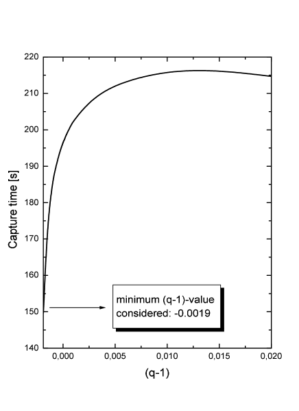
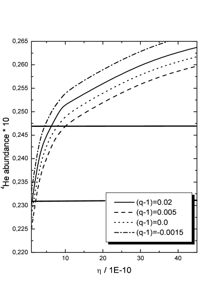
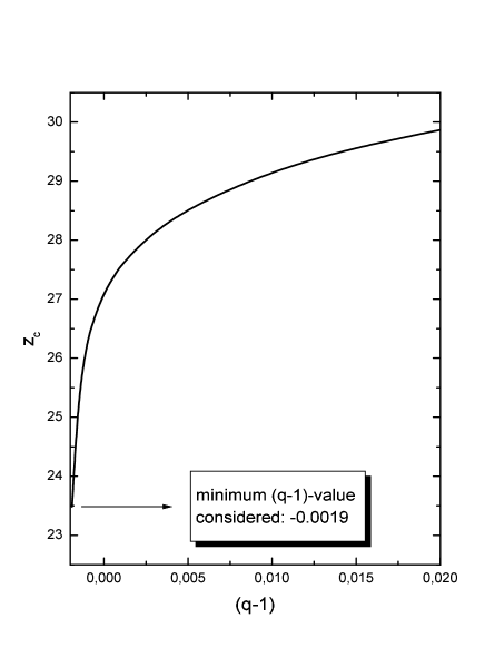
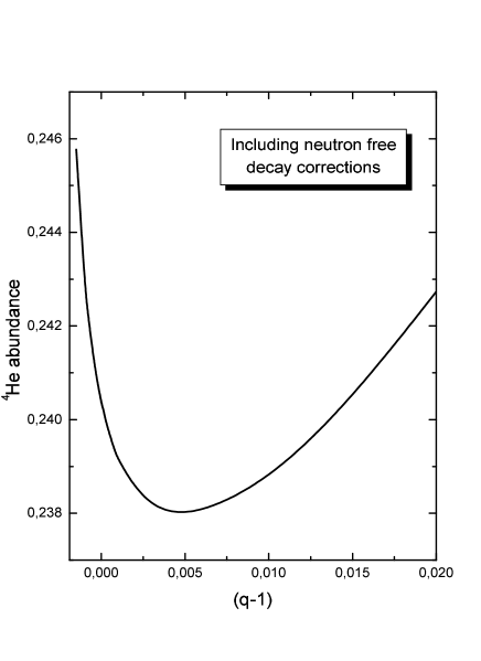
The standard result (i.e. (q1)=0𝑞10(q-1)=0) gives zc=27.08subscript𝑧𝑐27.08z_{c}=27.08. The numerical solution of this equation for different values of the parameter (q1)𝑞1(q-1), and the corresponding capture time, are shown in Fig. (7). It is interesting to notice that while values of (q1)>0𝑞10(q-1)>0 can be used within the analytical study presented in this Section without any limit, this is not the case for values of the parameter such that (q1)<0𝑞10(q-1)<0. The problem arises in that in these cases, Gnpqsubscriptsuperscript𝐺𝑞𝑛𝑝G^{q}_{np} can become negative, what clearly has no sense. In particular, for (q1)=0.002𝑞10.002(q-1)=-0.002, the denominator in Eq. (107) is identically zero, while for values of (q1)<0.002𝑞10.002(q-1)<-0.002 it is negative. Although this mines the physical viability of the description for these values of q𝑞q, in the same sense that what was referred before, other assumptions are taken in this Section, and only a numerical code can give a more precise answer in either way. Note that to obtain Fig. 7 we have made use of the non-extensive time-temperature correction. In Fig. 8 (left panel), we show the dependence of the 4He abundance as a function of (q1)𝑞1(q-1), taking into the free neutron decay correction.
Refer to caption
Refer to caption
Figure 7: Left: zcsubscript𝑧𝑐z_{c} as a function of (q1)𝑞1(q-1). Right: Capture time as a function of (q1)𝑞1(q-1). Both plots are constructed for a nominal value of ηq=3.57×10¹⁰subscript𝜂𝑞3.57superscript1010\eta_{q}=3.57\times 10^{-10}. Note the asymmetric range of the (q1)𝑞1(q-1)-values considered. See text for explanation.

Some comments about Figs. 7 and 8 are worth doing. Firstly, note that the dependence of the 4He abundance, when neutron free decay is taken into account, is no longer linear as it was before, see for instance Eq. (78). This makes the study of the nucleosynthesis process much more interesting, and the use of the full numerical code a worth doing task. Now we know that even when considering a first (linear) order correction in the quantum distribution functions, the final output in the primordial nucleosynthesis cannot be reduced to a linear correction in the abundances. Secondly, it appears that for a given value of Ypsubscript𝑌𝑝Y_{p} (and η𝜂\eta) there are two values of (q1)𝑞1(q-1) that could fit well the observations. Finally note that the y-axis of Fig. 8 (left panel) is showing variations at the level of less than 1%, and in principle, all values of (q1)𝑞1(q-1) shown there are admitted by the current constraints on the primordial abundance of 4He.
Refer to caption
Refer to caption
Figure 8: Left: 4He abundance as a function of (q1)𝑞1(q-1), taking into account neutron decay corrections. This plot is constructed for a nominal value of ηq=3.57×10¹⁰subscript𝜂𝑞3.57superscript1010\eta_{q}=3.57\times 10^{-10}. Right: Primordial abundance of 4He as a function of ηqsubscript𝜂𝑞\eta_{q}. Several (q1)𝑞1(q-1)-values are shown. Two horizontal lines stand for a conservative current constraint on Ypsubscript𝑌𝑝Y_{p}.

In Fig. 8 (right panel) we show for the first time the dependence of the 4He abundance as a function of ηqsubscript𝜂𝑞\eta_{q}, for different (q1)𝑞1(q-1)-values. The general trend of an increasing abundance as a function of η𝜂\eta is maintained, but for different values of q𝑞q, the curves cross the current constraints in different positions. This plot actually represents a 3D problem, with a two parameter space. The influence of η𝜂\eta appears when numerically solving the equation for zcsubscript𝑧𝑐z_{c}. Indeed, the computation of the correction to the value of Ypsubscript𝑌𝑝Y_{p} in the full analytical treatment presented here has to take into account different contributions. A direct linear dependence on (q1)𝑞1(q-1) is within the time-temperature relationship (see the first equations in this section, especially Eq. (83)) and in Eq. (78). In addition, we can see that if zcsubscript𝑧𝑐z_{c} is smaller than in the standard case, then Tcsubscript𝑇𝑐T_{c} will be bigger, and tcsubscript𝑡𝑐t_{c} will be smaller than their respective standard counterparts. Thus, et/τsuperscript𝑒𝑡𝜏e^{-t/\tau} will in turn be bigger, what happens for instance in the case of a negative value of (q1)𝑞1(q-1), and this would provide a bigger Ypsubscript𝑌𝑝Y_{p}. However, the linear correction in Eq. (78) is competing with that positive deviation; this is what finally makes the curve to deviate from a straight line.

10 Conclusions

In this paper, based on previous works (Paper I), we have revisited the problem of the primordial genesis of light elements within the framework of non-extensive statistics. We have particularly paid attention to the form of the principle of detailed balance that is valid in this new setting. We have shown that its usual form is no longer valid, but instead, that it is just an approximation, dubbed here as the BST. The full, new form of the principle of detailed balance was derived and named as BNE, and we have studied it in detail too. By doing so, we were able to disguise the range of validity of previous approaches to the topic, and to formally see the origin and range of the deviations between the standard and non-extensive scenarios for the primordial production of elements. We have also analyzed the neutron free decay correction to the capture time, and found that even when considering a first (linear) order correction in the quantum distribution functions, the final output cannot be reduced to a linear correction in the abundances, as Fig. 8 explicitly show. By comparing with the latest observational data, we have obtained a new bound on the upper limit of the parameter |q1|𝑞1|q-1|. We think that the bound being presented here (referring also to Figs. 7 and 8) is obtained within a much more detailed basis than the previous ones, see for instance [2, 3, 4], and then that this bound should be considered as the more reliable of them all. Indeed, we believe that the only way to improve it is to go to a direct implementation of the primordial nucleosynthesis code. By doing so we would have the possibility of studying the modifications to the abundances of all light elements in a simultaneous way. This further extension is currently under analysis.

Appendix: un+upuDsubscript𝑢𝑛subscript𝑢𝑝subscript𝑢𝐷u_{n}+u_{p}-u_{D}

To have a rough idea of the order of magnitude of the function un+upuDsubscript𝑢𝑛subscript𝑢𝑝subscript𝑢𝐷u_{n}+u_{p}-u_{D}, we need to compute (miμi)/Tsubscript𝑚𝑖subscript𝜇𝑖𝑇(m_{i}-\mu_{i})/T in the range of temperatures we are interested in, with i=n,p,𝑖𝑛𝑝i=n,p, and D𝐷D. Firstly, we note that for this purpose it is enough to consider the standard values of all these quantities. This is because non-extensive effects here would introduce only second order corrections in (q1)𝑞1(q-1), that we are disregarding in our computation. Recalling the relation Xi=(gi/nB)(miT/2π)3/2exp((miμi)/T)subscript𝑋𝑖subscript𝑔𝑖subscript𝑛𝐵superscriptsubscript𝑚𝑖𝑇2𝜋32𝑒𝑥𝑝subscript𝑚𝑖subscript𝜇𝑖𝑇X_{i}=(g_{i}/n_{B})(m_{i}T/2\pi)^{3/2}exp((m_{i}-\mu_{i})/T), we see that in order to estimate the values of (miμi)/Tsubscript𝑚𝑖subscript𝜇𝑖𝑇(m_{i}-\mu_{i})/T we need to know the abundances Xisubscript𝑋𝑖X_{i}. Then, to get un+upuDsubscript𝑢𝑛subscript𝑢𝑝subscript𝑢𝐷u_{n}+u_{p}-u_{D}, we have made the following steps:

  1. 1.

    Using the time-temperature relation we can put Xn(t)=exp(τ/t)Xn(tfrezee)subscript𝑋𝑛𝑡𝑒𝑥𝑝𝜏𝑡subscript𝑋𝑛subscript𝑡𝑓𝑟𝑒𝑧𝑒𝑒X_{n}(t)=exp(-\tau/t)X_{n}(t_{frezee}) as an explicit function of T𝑇T. Thus Xn(T)subscript𝑋𝑛𝑇X_{n}(T) follows, as well as (mnμn)/Tsubscript𝑚𝑛subscript𝜇𝑛𝑇(m_{n}-\mu_{n})/T.

  2. 2.

    Considering Xn(T)subscript𝑋𝑛𝑇X_{n}(T) together with the obtainable function XnXp/XDsubscript𝑋𝑛subscript𝑋𝑝subscript𝑋𝐷X_{n}X_{p}/X_{D} (remember that μn+μpμD=0subscript𝜇𝑛subscript𝜇𝑝subscript𝜇𝐷0\mu_{n}+\mu_{p}-\mu_{D}=0), and imposing the (approximate) constrain Xn+Xp+2XD=1subscript𝑋𝑛subscript𝑋𝑝2subscript𝑋𝐷1X_{n}+X_{p}+2X_{D}=1, we get the values of Xpsubscript𝑋𝑝X_{p} and XDsubscript𝑋𝐷X_{D}. Then, the corresponding values of (mpμp)/Tsubscript𝑚𝑝subscript𝜇𝑝𝑇(m_{p}-\mu_{p})/T and (mDμD)/Tsubscript𝑚𝐷subscript𝜇𝐷𝑇(m_{D}-\mu_{D})/T can be obtained.

These results allow us to construct un+upuDsubscript𝑢𝑛subscript𝑢𝑝subscript𝑢𝐷u_{n}+u_{p}-u_{D} and thus to see that 103superscript10310^{3} constitutes an upper bound in the range 0.070.070.07MeV <T<0.1absent𝑇0.1<T<0.1MeV (i.e. 22<z<3222𝑧3222<z<32).

Acknowledgments

M. E. Pessah is supported by Fundación Antorchas. We thank A. Lavagno, G. Lambiase, P. Quarati, and H. Vucetich for valuable discussions. D. F. T. was supported by CONICET as well as by funds granted by Fundación Antorchas, and acknowledges the hospitality provided by the Politecnico di Torino, the University of Salerno, and the ICTP (Italy) during different stages of this research.

References

  • [1] M. E. Pessah, D. F. Torres and H. Vucetich, Paper I, Physica A, this same issue.
  • [2] D. F. Torres, H. Vucetich and A. Plastino, Phys. Rev, Lett. 79, 1588 (1997); E80, 3889 (1998).
  • [3] D. F. Torres and H. Vucetich, Physica A259, 397 (1998).
  • [4] U. Tırnaklı and D. F. Torres, Physica A268, 225 (1999).
  • [5] L. Cucurull, J. A. Grifols and R. Toldrá, Astroparticle Phys. 4, 391 (1996).
  • [6] J. Bernstein, L. S. Brown and G. Feimberg, Rev. Mod. Phys. 61, 25 (1989). 397 (1998).
  • [7] S. Weimberg, Gravitation and Cosmology (John Wiley, New York, 1972).
  • [8] V. H. Hamity and D. E. Barraco, Phys. Rev. Lett. 76, 25 (1996).
  • [9] J. Peacock, Cosmological Physics (Cambridge University Press, Cambridge, 1999).
  • [10] S. Beuler, K. M. Nollett and M. S. Turner, astro-ph/0008495; S. Espósito, G. Mangano, G. Miele and O. Pisanti, astro-ph/9907422.
  • [11] P. Peebles, Principles of Physical Cosmology (Princeton University Press, Princeton, 1993)