Multi-vehicle Cooperative Control Using Mixed Integer Linear Programming
Abstract
We present methods to synthesize cooperative strategies for multi-vehicle control problems using mixed integer linear programming. Complex multi-vehicle control problems are expressed as mixed logical dynamical systems. Optimal strategies for these systems are then solved for using mixed integer linear programming. We motivate the methods on problems derived from an adversarial game between two teams of robots called RoboFlag. We assume the strategy for one team is fixed and governed by state machines. The strategy for the other team is generated using our methods. Finally, we perform an average case computational complexity study on our approach.
Index Terms:
Cooperative robotics, multi-vehicle systems, mixed integer linear programming, robot motion planning, path and trajectory planning, hybrid systems, mathematical optimization.I Introduction
For many problems, a team of vehicles can accomplish an objective more efficiently and more effectively than a single vehicle can. Some examples include target intercept [2], search [4], terrain mapping [24], object manipulation [38], surveillance, and space-based interferometry. For these problems, it is desirable to design a multi-vehicle cooperative control strategy.
There is a large literature on cooperative control. Work from team theory [25, 21] considers the case where team members have different information and the objective function is quadratic. Cooperative estimation for reconnaissance problems is considered in [30]. In [32, 6, 16] mixed integer linear programming is used for multi-vehicle target assignment and intercept problems. Hierarchical methods are used for cooperative rendezvous in [27] and for target assignment and intercept in [2]. A review from the machine learning perspective is presented in [35]. There are several recent compilations of cooperative control articles in [1, 5, 28].
In this paper, we propose a hybrid systems approach for modeling and cooperative control of multi-vehicle systems. We use the class of hybrid systems called mixed logical dynamical systems [7], which are governed by difference equations and logical rules and are subject to linear inequality constraints. The main motivation for using mixed logical dynamical systems is their ability to model a wide variety of multi-vehicle problems and the ease of modifying problem formulations. In our approach, a problem is modeled as a mixed logical dynamical system, which we represent as a mixed integer linear program (MILP). Then, to generate a cooperative control strategy for the system, the MILP is solved using AMPL [19] and CPLEX [22].
Posing a multi-vehicle control problem in a MILP framework involves modeling the vehicle dynamics and constraints, modeling the environment, and expressing the objective. To demonstrate the modeling procedure and our approach, we consider control problems involving Cornell’s multi-vehicle system called RoboFlag. For an introduction to RoboFlag, see the papers from the invited session on RoboFlag in the Proceedings of the 2003 American Control Conference [10, 12, 13].
Our focus is to find optimal solutions using a flexible methodology, which is why we use MILP. However, because MILP is in the NP-hard computation class [20], the methods may not be fast enough for real-time control of systems with large problem formulations. In this case, the methods can be used to explore optimal cooperative behavior and as benchmarks to evaluate the performance of heuristic or approximate methods. In Section VI, we discuss several methods for reducing the computational requirements of our MILP approach so that it can be more readily used in real-time applications.
Our approach for multi-vehicle control, first presented in [15, 16], was developed independently from a similar approach developed by Richards et. al. [33]. Next, we list some of the noteworthy aspects of our approach. First, the environment which we demonstrate our methods involves an adversarial component. We model the intelligence of the adversaries with state machines. Second, our approach allows multiple, possibly nonuniform, time discretizations. Discretizing continuous variables in time is necessary for MILP formulations. Using many time steps results in large MILPs that require a considerable amount of computation time to solve. Support for nonuniform discretizations in time allows the use of intelligent time step selection algorithms for the generation of more efficient MILP problem formulations [17]. Finally, because we include the vehicle dynamics in the problem formulation, the resulting trajectories are feasible, which is advantageous because they can be applied directly to the multi-vehicle system. In order to express the vehicle dynamics efficiently in our MILP formulation, we restrict the control input to each vehicle in a way that allows near-optimal performance, as presented in [29].
The paper is organized as follows: First, we consider vehicle problems that have relatively simple formulations. Then we add features in each section until we arrive at the RoboFlag multi-vehicle problems. In Section II, we introduce the dynamics of the vehicles used to motivate our approach, and we formulate and solve a single vehicle minimum control effort trajectory generation problem. We build upon this in Section III adding obstacles that must be avoided. In Section IV, we show how to generate optimal team strategies for RoboFlag problems. In Section V, we perform an average case computational complexity study on our approach. Finally, in Section VI, we discuss our methods and ways in which they can be be applied. All files for generating the plots found in this paper are available online [18].
II Vehicle dynamics
Multi-vehicle control problems involving the wheeled robots of Cornell’s RoboCup Team [14, 37] are used to motivate the methods presented in this paper. In this section, we show how to simplify their nonlinear governing equations using a procedure from [29]. The result is a linear set of governing equations coupled by a nonlinear constraint on the control input, which admits feasible vehicle trajectories and allows near-optimal performance. We then show how to represent the simplified system in a MILP problem formulation.
Each vehicle has a three-motor omni-directional drive, which allows it to move along any direction irrespective of its orientation. The nondimensional governing equations of each vehicle are given by
| (1) |
where ,
| (2) |
and . In these equations, are the coordinates of the vehicle on the playing field, is the orientation of the vehicle, is the -dependent control input, is the mass of the vehicle, is the vehicle’s moment of inertia, is the distance from the drive to the center of mass, and is the voltage applied to motor . The set of admissible voltages is given by the unit cube, and the set of admissible control inputs is given by .
These governing equations are coupled and nonlinear. To simplify them, we replace the set with the maximal -independent set found by taking the intersection of all possible sets of admissible controls. The result is a -independent control input, denoted , that is subject to the inequality constraints and .
Using the restricted set as the set of allowable control inputs, the governing equations decouple and are given by
| (3) |
The constraints on the control input couple the degrees of freedom.
To decouple the dynamics, we set . Then the constraint on the control input becomes
| (4) |
Now the equations of motion for the translational dynamics of the vehicle are given by
| (5) |
subject to equation (4). In state space form, equation (II) is , where is the state and is the control input.
By restricting the admissible control inputs we have simplified the governing equations in a way that allows near optimal performance as shown in [29]. This procedure allows real-time calculation of many near-optimal trajectories and has been successfully used by Cornell’s RoboCup team [14, 37, 29].
To represent the governing equations in a MILP framework, we discretize the control input in time and require it be constant between time steps. The result is a set of linear discrete time governing equations.
Let be the number of discretization steps for the control input , let be the time at step , and let be the time between steps and , for . The discrete time governing equations are given by
| (6) |
where , ,
| (11) |
| (16) |
, and . The coefficients and are functions of because we have allowed for nonuniform time discretizations. Because there will be several different time discretizations used in this paper, we use subscripts to differentiate them. In this section, we use the subscript to denote variables associated with the discretization in the control input .
The discrete time governing equations can be solved explicitly to obtain
and similarly for and .
In later sections of this paper it will be necessary to represent the position of the vehicle at times between control discretization steps, in terms of the control input. Because the set of governing equations is linear, given the discrete state and the control input , we can calculate the vehicle’s state at any time using the following equations:
| (17) |
where satisfies . If the time discretization of the control input is uniform, for all , then . The other components of the vehicle’s state, and , can be calculated in a similar way.
The control input constraint given by equation (4) cannot be expressed in a MILP framework because it is nonlinear. To incorporate this constraint we approximate it with a set of linear inequalities that define a polygon. The polygon inscribes the region defined by the nonlinear constraint. We take the conservative inscribing polygon to guarantee that the set of allowable controls, defined by the region, is feasible. We define the polygon by the set of linear inequality constraints
| (18) |
for each step .
To illustrate the approach, we consider the following minimum control effort trajectory generation problem. Given a vehicle governed by equations (6) and (18), find the sequence of control inputs that transfers the vehicle from starting state to finishing state and minimizes the cost function
| (19) |
To convert the absolute values in the cost function to linear form, we introduce auxiliary continuous variables and and the inequality constraints
| (20) |
Minimizing subject to the inequalities and is equivalent to minimizing (similarly for . Using the auxiliary variables, the cost function can be written as a linear function,
| (21) |
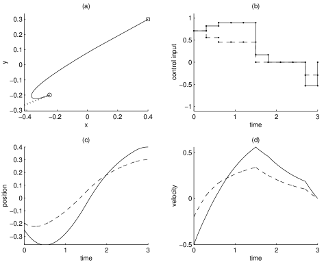
The resulting optimization problem (minimize (21) subject to (6), (18), (20), and the boundary conditions) is in MILP form. Because binary variables do not appear in the problem formulation, it is a linear program and is easily solved to obtain the optimal sequence of control inputs. The solution for an example instance is shown in Figure 1.
III Obstacle avoidance
In vehicle control, it is necessary to avoid other vehicles, stationary and moving obstacles, and restricted regions. In this section, we show how to formulate and solve these avoidance problems using MILP. We start by showing a MILP method to guarantee circular obstacle avoidance at discrete times. The version of this method developed in [34], and a similar version developed independently in in [15, 16], uniformly distributes obstacle avoidance times. Here we present a version of the method that allows nonuniform distributions of obstacle avoidance times.
The subscript is used to denote variables associated with the time discretization for obstacle avoidance. For step , taken to be an element of the set , let be the time at which obstacle avoidance is enforced. Let denote the radius of the obstacle. Let denote the coordinates of its center at time . We approximate the obstacle with a polygon, denoted , defined by a set of inequalities. The polygon is given by
| (22) | |||||
To guarantee obstacle avoidance at time , the coordinates of the vehicle must be outside the region . This avoidance condition can be written as , where are the coordinates of the vehicle at time . Here and are expressed in terms of the control inputs using equation (17).
Because at least one constraint defining the region must be violated in order to avoid the obstacle, the avoidance condition is equivalent to the following condition:
| (23) |
To express this avoidance constraint in a MILP problem formulation, it must be converted to an equivalent set of linear inequality constraints. We do so by introducing auxiliary binary variable and the following inequality constraints,
| (24) |
where is a large positive number taken to be larger than the maximum dimension of the vehicle’s operating environment plus the radius of the obstacle. If , the right hand side of the inequality is a large, negative number that is always less than the left hand side. In this case, the inequality is inactive because it is trivially satisfied. If , the inequality is said to be active because it reduces to an inequality from the existence condition above. For obstacle avoidance, at least one of the constraints in equation (III) must be active. To enforce this, we introduce the following inequality constraint into the problem formulation,
| (25) |
Therefore, to enforce obstacle avoidance at time , the set of binary variables and the constraints given by equations (III) and (25) are added to the MILP problem formulation.
Consider the example problem from Section II with obstacles. In this problem, we want to transfer the vehicle from start state to finish state in time using minimal control effort while avoiding obstacles. To enforce obstacle avoidance at each time in the set , we augment the MILP formulation in Section II with the set of binary variables , constraints (III), and constraint (25) for all in the set .
Distributing the avoidance times uniformly (uniform gridding), as in [34, 16], results in a trajectory that avoids obstacles at each discrete time in the set, but the trajectory can collide with obstacles between avoidance times. This is shown for an example instance in Figure 2(a). In this example, the trajectory intersects the obstacle between the sixth and seventh avoidance time steps. A simple method to eliminate this behavior is to represent the obstacle with a polygon that is larger than the obstacle. Then distribute obstacle avoidance times uniformly such that the sampling time is small enough to guarantee avoidance. In general, this is not a desirable approach because it results in large MILPs that require significant computational effort to solve.
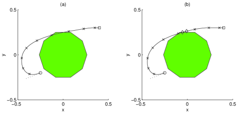
A better approach is to select the avoidance times intelligently. In [17], we have developed an iterative MILP algorithm that does this. We summarize this algorithm here. First, pick an initial set of times at which obstacle avoidance will be enforced. Then, formulate and solve the MILP as described above representing the obstacles with polygons slightly larger than the obstacles. Next, check the resulting trajectory for collisions with any of the obstacles (not the polygons which represent them in the MILP). If there are no collisions, terminate the algorithm. If there is a collision, compute the time intervals for which collisions occur denoting the time interval for collision by . For each interval , pick a time within the interval, such as . At each of these times add obstacle avoidance constraints to the MILP formulation. Then, solve the augmented MILP repeating the procedure above (first checking if the resulting trajectory intersects any obstacles, etc.) until a collision free trajectory is found. Figure 2(b) shows the effectiveness of this algorithm after two iterations.
IV RoboFlag Problems
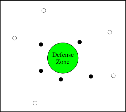
To motivate our multi-vehicle methods, we apply them to simplified versions of the RoboFlag game [12, 13, 10], which we call RoboFlag Drills because they serve as practice for the real game. The drills involve two teams of robots, the defenders and the attackers, on a playing field with a circular region of radius at its center called the Defense Zone, as shown in Figure 3. The attackers’ objective is to fill the Defense Zone with as many attackers as possible. The defenders’ objective is to deny as many attackers from entering the Defense Zone as possible without entering the zone themselves. We consider Defensive Drill problems in which each attacker has a fixed intelligence governed by a state machine. The goal is to design a team control strategy for the defenders that maximizes the number of attackers denied from the Defense Zone. In this section, we use MILP methods to generate such strategies. We consider two versions of the Defensive Drill each with a different set of laws governing attacker intelligence.
To start, we consider one-on-one Defensive Drill problems. This is the simplest case and involves one defender and one attacker. Although this case is not particularly interesting, we start with it for notational clarity. Next, we generalize to the case involving defenders and attackers, which is a straightforward extension.
IV-A Defensive Drill 1: one-on-one case
The defender is governed by the discrete time dynamical system from Section II
| (26) |
The attacker has two discrete modes: attack and inactive. When in attack mode, it moves toward the Defense Zone at constant velocity along a straight line path. The attacker, initially in attack mode at the beginning of play, transitions to inactive mode if the defender intercepts it or if it enters the Defense Zone. Once inactive, the attacker does not move and remains inactive for the remainder of play. These dynamics are captured by the following discrete time equations and state machine
| (27) |
| (34) | |||

with initial conditions
| (35) |
where is the number of samples, ,
is the time between samples and , is
the attacker’s position at time ,
is its constant velocity vector, and
is a discrete state indicating the attacker’s mode. The attacker is
in attack mode when and inactive mode when .
The attacker state machine is shown in Figure 4. Here we use the
subscript to denote the time discretization for the attacker’s
dynamics.
Defense Zone
Because the defender wants to keep the attacker from entering the Defense Zone, a binary variable indicating whether or not the attacker is inside the Defense Zone is introduced. This variable is used to define the attacker state machine precisely. We denote the binary variable with . When the attacker is in the Defense Zone at step , . When the attacker is outside the Defense Zone at step , .
Similar to the approach used to define obstacles, the Defense Zone is approximated using a polygon defined by a set of inequalities
| (36) | |||||
The association between and is
| (37) |
If the defender keeps the binary variable equal to for all , it has successfully denied the attacker from the region and thus from the Defense Zone. However, in order to use the binary variable in the problem formulation, we must enforce the logical constraint given by equation (37). To enforce this constraint in MILP, we convert it into an equivalent set of inequality constraints.
We introduce the binary variable to indicate whether or not the th constraint of is satisfied by the attacker with position . This association is made by introducing the logical constraint
| (38) |
As shown in Appendix A, it is equivalent to the following set of inequalities
| (39) |
where is a small positive number and is a large positive number such that the left hand sides of the inequalities are bounded from above by and from below by .
Using binary variable , we can write equation (37) as
| (40) |
which is equivalent to the inequality constraints
| (41) |
as shown in Appendix A.
The logical constraint given by equation (37) is equivalent
to the inequality constraints given by equations (39)
and (41). Therefore, we can include the indicator
variable in the MILP formulation by also including the binary
variables and constraints (39)
and (41).
Intercept Region
To define what it means for a defender to intercept an attacker, we introduce an intercept region rigidly attached to the defending robot. The intercept region is a polygon defined by a set of inequalities. If an attacker is in this polygon, it is considered intercepted. For the defender with coordinates , the intercept region is given by
| (42) | |||||
where and are calculated using equation (17), and is the inscribed radius of the polygon.
The binary variable is introduced to indicate whether or not the attacker is inside the defender’s intercept region. The association is made with the following logical constraint
| (43) |
Using techniques similar to those used for , we convert this constraint into an equivalent set of inequality constraints as follows: For each of the inequalities defining the intercept region, we associate a binary variable by introducing the logical constraint
| (44) |
where are the coordinates of the attacking robot. If , the coordinates of the attacking robot satisfy the th inequality defining the intercept region. If , the th inequality is not satisfied. Similar to equation (IV-A), we can express this logic constraint as the set of inequalities
| (45) |
Using the binary variables we can write equation (43) as
| (46) |
Considering both directions of this equivalence, as done for above, we find that the statement is equivalent to the following set of inequality constraints
| (47) |
We can use in our problem formulation if we include the
binary variables and the inequalities
constraints given by equations (45)
and (47).
State machine and objective function
With the indicator variables and defined, we revisit the attacker state machine and define it more precisely with the following state equation

| (52) |
which is shown in Figure 5. The state equations can be written as the logical expression
| (53) |
which is equivalent to the set of inequality constraints
| (54) |
as shown in Appendix A.
We have defined the dynamics of the defenders and the attackers, and we have converted these dynamics to MILP form. The final step in formulating Defensive Drill 1 is to introduce an objective function that captures the defender’s desire to deny the attacker from entering the Defense Zone. This objective is achieved by minimizing the binary variable over the duration of the drill, which is captured by minimizing the function
| (55) |
We set the duration of the drill such that
| (56) |
This allows the attacker enough time to reach the Defense Zone if it is not intercepted.
In addition to intercepting the attacker, we would like to conserve fuel as a secondary objective. One way to achieve this is to add a small penalty on the control effort to the objective function as follows:
| (57) |
where is taken to be a small positive number because we
want the minimization of the binary variable to dominate.
We use the procedure outlined in Section II to
write equation (57) in MILP form.
Summary and example
We have formulated Defensive Drill 1 as the following optimization problem: minimize (57) subject to defender dynamics (26); attacker dynamics (27), (35), and (54) for all ; the constraints for the indicator variable (39) and (41) for all and for all ; the constraints for the indicator variable (45), and (47) for all and for all ; and the avoidance constraints for the Defense Zone (III) and (25) for all and for all .
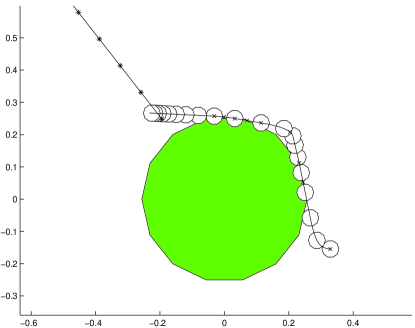
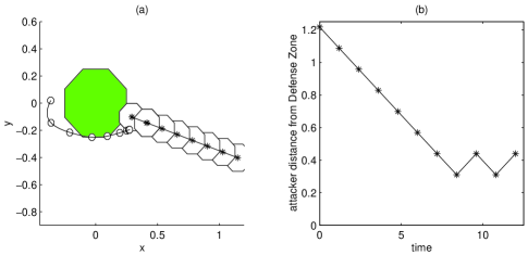
The solution to an instance of this problem is shown in Figure 6. For this instance, the defender denies the attacker from the Defense Zone (shaded polygon) by intercepting it. Each asterisk along the attacker’s trajectory denotes the position of the attacker at sample time . The white polygons along the defender’s trajectory denotes the intercept region at time .
IV-B Defensive Drill 2: one-on-one case

The dynamics of the defender are the same as the defender dynamics in Section IV-A. The dynamics of the attacker are the same as the attacker dynamics in Defensive Drill 1, but with an additional state called retreat. If a defender is too close to the attacker, the attacker enters the retreat state and reverses direction. While retreating, if the defender is far enough away, the attacker returns to attack mode.
These dynamics are captured by the following discrete time equations and state machine:
| (58) |
| (65) | |||
| (72) |
for all and subject to the constraint
| (73) |
and the initial conditions
| (74) |
The state machine is shown in Figure 7.
The attacker needs two binary state variables because it has three discrete modes of operation: attack, retreat, and inactive. These modes are represented by , , and , respectively. Because the state is not needed, we impose the inequality constraint given by equation (73).
To determine if the defender is too close to the attacker, a warning region is introduced. The warning region is a polygon defined by a set of inequalities similar to the intercept region . We introduce binary auxiliary variables and , and we introduce inequality constraints similar to equations (45) and (47). The result is the following association for indicator variable : If , the defender is in the attacker’s warning region at step , otherwise, . The attacker state machine can be written as the set of inequality constraints
| (75) |
Similar to Defense Drill 1, Defense Drill 2 can be posed as a MILP. The solution of an example instance is shown in Figure 8.
IV-C -on- case
To generalize the problem formulation to defenders and attackers, we need to add more variables. Defender , where , has state , control input , and slack variables and . Attacker , where , has state and constant velocity vector . The binary variable equals if and only if attacker is in polygon at step . The binary variable equals if and only if attacker is in defender ’s intercept region at step . The binary variables , , and follow a similar trend. For Defensive Drill 2, we also need if and only if defender is in attacker ’s warning region at step . And similarly for the binary variable .
With the variables for the general case defined, inequality constraints are added to the formulation in a similar way as those derived for the one-on-one case. For example, the constraints identifying with are
for all and for all .
And finally, the objective function is given by
| (76) |
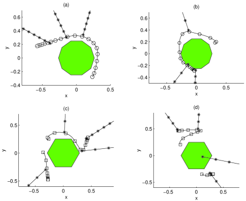
Results for example instances of Defensive Drill 1 are shown in Figure 9.
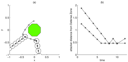
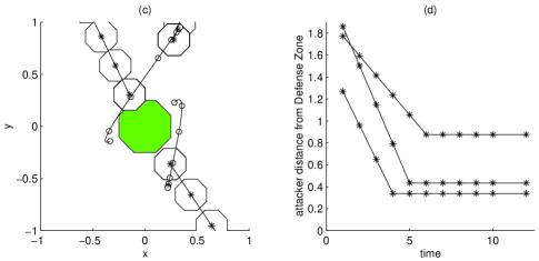
Results for Defensive Drill 2 are shown in Figure 10.
V Average case complexity
In this section, we explore the average case complexity of Defensive Drill 1 by solving randomly generated instances. Each instance is generated by randomly picking parameters from a uniform distribution over the intervals defined below. Each MILP is solved using AMPL [19] and CPLEX [22] on a PC with Intel PIII 550MHz processor, 1024KB cache, 3.8GB RAM, and Red Hat Linux. For all instances solved, processor speed was the limiting factor, not memory.
To generate the initial condition and the constant velocity vector for each attacker we pick , , and randomly from a uniform distribution over the intervals , , and , respectively. The parameters are then given by
| (77) |
To generate the initial condition for each defender, we pick , , , and randomly from a uniform distribution over the intervals , , , and , respectively. The defender’s initial condition is then given by
| (78) |
We take the playing field to be circular with radius , and we set the radius of the Defense Zone to be . The intervals used to generate the instances are , , and . We take the attacker velocity to be .
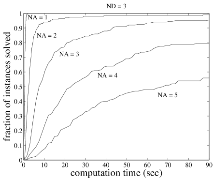
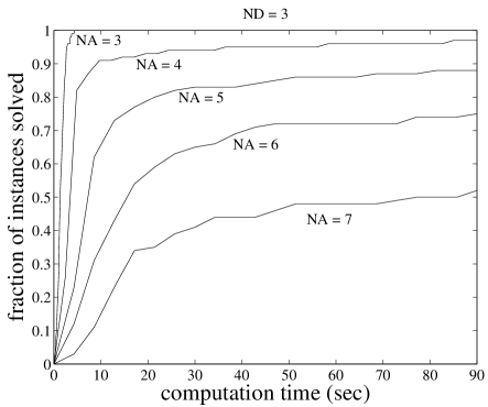
In Figure 11, we plot the fraction of instances solved versus computation time for the case where the cost function includes the number of attackers that enter the Defense Zone plus a penalty on the control effort. This cost function is given by equation (76) with . In Figure 12, we plot the fraction of instances solved versus computation time for the case where the cost function includes only the number of attackers that enter the Defense Zone. This cost function is given by equation (76) with .
As these figures show, the case where the cost function only includes the number of attackers that enter the Defense Zone is less computationally intensive than the case where the cost function also includes a penalty on the control effort. For example, for the case where , , and , 50% of the problems are solved in 3.5 seconds. However, for the case where , , and , 50% of the problems are solved in 78 seconds.
When in the cost function, the solver stops once a set of trajectories for the defenders is found that results in the minimum number of attackers entering the Defense Zone. This trajectory is often not the most efficient trajectory with respect to the control effort of the defenders. For the case where , once a set of defender trajectories is found that results in the minimum number of attackers entering the Defense Zone the solver continues to search. The solver searches until it finds a set of defender trajectories that not only results in the minimum number of attackers entering the Defense Zone but also uses the defender control effort in the most efficient way.
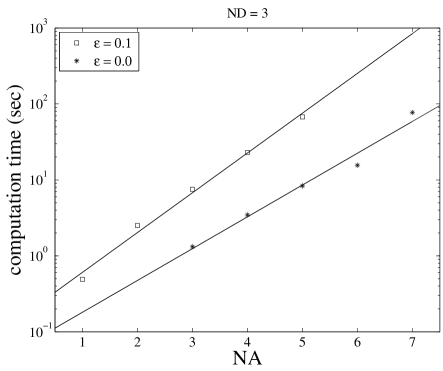
In Figure 13, we plot the computation time necessary to solve 50% of the randomly generated instances versus the size of the attacker set. For all instances considered, the defender set is of constant size (). We plot the data for both cost functions considered above ( and ). This figure shows that the computation time grows exponentially with the number of vehicles in the attacker set.
VI Discussion
In this paper, we showed how to use MILPs to model and generate strategies for multi-vehicle control problems. The MILP formulation is very expressive and allows all aspects of the problem to be taken into account. This includes the dynamic equations governing the vehicles, the dynamic equations governing the environment, the state machine governing adversary intelligence, logical constraints, and inequality constraints. The solution to the resulting MILP is the optimal team strategy for the problem. As shown by our average case complexity study, the MILP method becomes computational burdensome for large problems and thus, for these cases, is not suitable for real-time applications.
There are several steps that can be taken to make the MILP approach applicable for real-time multi-vehicle control applications. One approach is to solve the MILPs faster. This can be done by using a more powerful computer or by distributing the computation over a set of processors. For the multi-vehicle control problems, it may be advantageous to distribute the computation over the set of vehicles. Distributed methods for solving MILPs have been considered in [31].
Another approach is to move all, or some components of, the computational burden offline. This can be done by formulating the problem as a multi-parametric MILP. A multi-parametric MILP is a MILP formulated using a set of parameters each allowed to take on values over an interval. This problem is much more computationally intensive than the MILP problems considered in this paper. However, because the computation is performed offline, this is not an issue unless the computation takes an unreasonable amount of time. With the solution to the multi-parametric MILP, a table can be formed and used to look up optimal team strategies for the multi-vehicle system in real time. Multi-parametric MILP control problems can be solved using the Multi-Parametric Toolbox [23].
Finally, we discuss efficient MILP formulations as a way of decreasing computational requirements. The computational effort required to solve a MILP depends most on the number of binary variables used in its MILP problem formulation. Thus, reducing the number of binary variables is advantageous. In this paper, our motivating problem required three different time discretizations. The discretizations included one for the control input to the vehicles, one for obstacle avoidance, and one for attacker intercept. With each discretization step, a set of binary variables must be added to the MILP formulation. In most of the instances solved in this paper, we discretized time uniformly. However, we posed the MILP in a general way such that nonuniform time discretizations could be used. This allows for intelligent time distribution selection, which can significantly reduce the required computational effort to solve a problem. In [17], we developed several iterative MILP techniques for intelligent discretization step selection.
Appendix A
In this appendix, we illustrate how to convert a logic expression into an equivalent set of inequalities using the procedure from [40]. First the logic expression is converted into a conjunction of disjunctions, called conjunctive normal form (CNF), by applying tautologies. For example, let the variables be binary variables. The expression
| or | |||
| and or | |||
| and or or | (79) |
is in CNF.
Once we have converted the logic expression into CNF we can easily write each disjunction as an inequality constraint that must be satisfied in order for the disjunction to be true. For example, the second disjunction of equation (A), or , is true if and only if . Therefore, equation A is true if and only if the following inequalities hold
| (80) |
A-A Equation (40)
First consider the () direction of equation (40). Replacing implication with disjunction we have
| (81) |
and distributing the OR we have
| (82) |
which is equivalent to
| (83) |
This expression is in CNF, therefore it is equivalent to the following set of inequality constraints
| (84) |
Now consider the () direction of equation (40). Replacing implication with disjunction
| (85) |
and distributing the negation we have
| (86) |
which is equivalent to
| (87) |
This expression, which is a disjunction, is in CNF and therefore is equivalent to the following inequality
| (88) |
A-B Equation (53)
First consider the direction of equation (53). Replacing implication with the equivalent disjunction we have
| (89) |
and distributing OR over AND we have
| (90) |
Now that the expression is in CNF we can easily write it as a set of inequality constraints.
| (91) |
Now consider the other direction of equation (53). Replacing the implication with disjunction we have
| (92) |
and distributing the negation we have
| (93) |
this disjunction is equivalent to the flowing inequality
| (94) |
In summary, we have taken the governing equations for the attacker’s binary state (52) and derived an equivalent set of inequalities: (91) and (94) which can be simplified to the inequalities given by equation (54).
Acknowledgment
We thank J. Ousingsawat for helpful comments and encouragement.
References
- [1] R. C. Arkin and G. A. Bekey, Eds., “Special Issue on Robot Colonies,” Autonomous Robots, vol. 4(1), 1997.
- [2] R. W. Beard, T. W. McLain, M. A. Goodrich, and E.P. Anderson, “Coordinated Target Assignment and Intercept for Unmanned Air Vehicles,” IEEE Trans. Robot. Automat., vol. 18, pp. 991–922, Dec. 2002.
- [3] R. W. Beard and V. Stepanyan, “Information Consensus in Distributed Multiple Vehicle Coordinated Control,” Proc. IEEE Conf. Decision and Control, Maui, Hawaii, Dec. 2003, pp. 2029–2034.
- [4] R. W. Beard and T. W. McLain, “Multiple UAV Cooperative Search under Collision Avoidance and Limited Range Communication Constraints ,” Proc. IEEE Conf. Decision and Control, Maui, Hawaii, Dec. 2003, pp. 25–30.
- [5] T. Balch and L. E. Parker, Eds., “Special Issue on Heterogeneous Multirobot Systems,” Autonomous Robots, vol. 8(3), 2000.
- [6] J. S. Bellingham, M. Tillerson, M. Alighanbari, and J. P. How, “Cooperative Path Planning for Multiple UAVs in Dynamic and Uncertain Environments,” Proc. IEEE Conf. Decision and Control, Las Vegas, Nevada, Dec. 2002, pp. 2816–2822.
- [7] A. Bemporad and M. Morari, “Control of Systems Integrating Logic, Dynamics, and Constraints,” Automatica, vol. 35, pp. 407–428, Mar. 1999.
- [8] D. Bertsimas and J. N. Tsitsiklis, Introduction to Linear Optimization, Athena Scientific, Belmont, Massachusetts, 1997.
- [9] S. H. Breheny, R. D’Andrea, and J. C. Miller, “Using Airborne Vehicle-based Antenna Arrays to Improve Communications with UAV Clusters,” Proceedings. 42nd IEEE Conference on Decision and Control, Dec. 2003, pp. 4158–4162.
- [10] M. Campbell, R. D’Andrea, D. Schneider, A. Chaudhry, S. Waydo, J. Sullivan, J. Veverka, and A. Klochko, “RoboFlag Games Using Systems Based, Hierarchical Control,” Proceedings of the American Control Conference, June 4–6, 2003, pp. 661–666.
- [11] C. G. Cassandras and W. Li, “A Receding Horizon Approach for Solving Some Cooperative Control Problems,” Proc. IEEE Conf. Decision and Control, Las Vegas, Neveda, Dec. 2002, pp. 3760–3765.
- [12] R. D’Andrea and R. M. Murray, “The RoboFlag Competition,” Proceedings of the American Control Conference, June 4–6, 2003, pp. 650–655.
- [13] R. D’Andrea and M. Babish, “The RoboFlag Testbed,” Proceedings of the American Control Conference, June 4–6, 2003, pp. 656–660.
- [14] R. D’Andrea, T. Kalmár-Nagy, P. Ganguly, and M. Babish, “The Cornell RoboCup Team,” In G. Kraetzschmar, P. Stone, T. Balch Eds., Robot Soccer WorldCup IV, Lecture Notes in Artificial Intelligence, Springer, 2001.
- [15] M. G. Earl and R. D’Andrea, “A Study in Cooperative Control: The RoboFlag Drill,” Proceedings of the American Control Conference, Anchorage, Alaska May 8–10, 2002, pp. 1811–1812.
- [16] M. G. Earl and R. D’Andrea, “Modeling and Control of a Multi-agent System Using Mixed Integer Linear Programming,” Proc. IEEE Conf. Decision and Control, Las Vegas, Neveda, Dec. 2002, pp. 107–111.
- [17] M. G. Earl and R. D’Andrea, “Iterative MILP Methods for Vehicle Control Problems,” Proc. IEEE Conf. Decision and Control, Atlantis, Paradise Island, Bahamas, Dec. 2004.
- [18] All files for generating the plots found in this paper are available online at http://control.mae.cornell.edu/earl/milp1
- [19] R. Fourer, D. M. Gay, B. W. Kernighan, “AMPL–A Modeling Language for Mathematical Programming,” Danvers, Mass., Boyd & Fraser, 1993.
- [20] M. R. Garey and D. S. Johnson. Computers And Intractability: A guide to the Theory of NP-Completeness. W. H. Freeman and Company, 1979.
- [21] Y. Ho and K. Chu, “Team Decision Theory and Information Structures in Optimal Control Problems – Part 1,” IEEE Trans. Automatic Control, vol. AC-17, pp. 15–22, 1972.
- [22] ILOG AMPL CPLEX System Version 7.0 User’s Guide, 2000, http://www.ilog.com/products/cplex/.
- [23] M. Kvasnica, P. Grieder, M. Baoti’c, and M. Morari, “Multi Parametric Toolbox (MPT),” Hybrid Systems: Computation and Control, Lecture Notes in Computer Science, Volume 2993, Springer Verlag, Pennsylvania, Philadelphia, USA, March 2003, pp. 448–462, http://control.ee.ethz.ch/mpt.
- [24] M. Di Marco, A. Garulli, A. Giannitrapani, A. Vicino A, “Simultaneous Localization and Map Building for a Team of Cooperating Robots: A Set Membership Approach,” IEEE Transactions on Robotics and Automation, vol. 19 (2), pp. 238–249, Apr. 2003.
- [25] J. Marschak and R. Radner, Econonomic Theory of Teams. Yale University Press, 1972.
- [26] D. Q. Mayne, J. B. Rawlings, C. V. Rao, and P. O. M. Scokaert, “Constrained Model Predictive Control: Stability and Optimality,” Automatica, vol. 36, pp. 789–814, 2000.
- [27] T. W. McLain, P. R. Chandler, S. Rasmussen, and M. Pachter, “Cooperative Control of UAV Rendezvous,” Proc. American Control Conference, Arlington, VA, June 2001, pp. 2309–2314.
- [28] R. Murphey and P. M. Pardalos, Eds., Cooperative Control and Optimization, Boston: Kluwer Academic, 2002.
- [29] T. Kalmár-Nagy, R. D’Andrea, and P. Ganguly. “Near-Optimal Dynamic Trajectory Generation and Control of an Omnidirectional Vehicle,” Robotics and Autonomous Systems, vol. 46, pp. 47–64, 2004.
- [30] J. Ousingsawat and M. E. Campbell, “Establishing Optimal Trajectories for Multi-vehicle Reconnaissance,” AIAA Guidance, Navigation and Control Conference, 2004.
- [31] T. L. Ralphs, “Parallel Branch and Cut for Capacitated Vehicle Routing,” Parallel Computing, vol. 29(5), pp. 607–629, May 2003.
- [32] A. Richards, J. Bellingham, M. Tillerson, and J. How, “Co-ordination and Control of Multiple UAVs,” AIAA Conf. Guidance Navigation and Control, August 2002.
- [33] A. Richards and J. P. How, “Aircraft Trajectory Planning With Collision Avoidance Using Mixed Integer Linear Programming,” In Proc. American Control Conf., 2002.
- [34] A. Richards, T. Schouwenaars, J. P. How and E. Feron, “Spacecraft Trajectory Planning with Avoidance Constraints Using Mixed-Integer Linear Programming,” Journal of Guidance, Control, and Dynamics, Vol. 25, pp. 755–764, July–August 2002.
- [35] P. Stone and M. Veloso, “Multiagent Systems: A Survey from a Machine Learning Perspective,” Autonomous Robots, vol. 8, pp. 345–383, 2000.
- [36] P. Stone. Layered Learning in Multiagent Systems: A Winning Approach to Robotic Soccer. MIT Press, 2000.
- [37] P. Stone, M. Asada, T. Balch, R. D’Andrea, M. Fujita, B. Hengst, G. Kraetzschmar, P. Lima, N. Lau, H. Lund,D. Polani,P. Scerri, S. Tadokoro,T. Weigel, and G. Wyeth, “RoboCup-2000: The Fourth Robotic Soccer World Championships,” AI MAGAZINE, vol. 22(1), pp. 11–38, Spring 2001.
- [38] T. G. Sugar and V. Kumar, “Control of Cooperating Mobile Manipulators,” IEEE Transactions on Robotics and Automation, vol. 18 (1), pp. 94–103, Feb. 2002.
- [39] F. D. Torrisi, A. Bemporad, and D. Mignone. HYSDEL—A Language for Describing Hybrid Systems. Technical Report AUT00-03, ETH Zurich, 2000. http://control.ethz.ch/hybrid/hysdel
- [40] M. L. Tyler and M. Morari, “Propositional Logic in Control and Monitoring Problems,” Automatica, vol. 35, pp. 565-582, 1999.
- [41] H. P. Williams, Model Building in Mathematical Programming, John Wiley and Sons, Third Edition, 1993.