Language identification of controlled systems: Modelling, control and anomaly detection
Abstract
Formal language techniques have been used in the past to study autonomous dynamical systems. However, for controlled systems, new features are needed to distinguish between information generated by the system and input control. We show how the modelling framework for controlled dynamical systems leads naturally to a formulation in terms of context-dependent grammars. A learning algorithm is proposed for on-line generation of the grammar productions, this formulation being then used for modelling, control and anomaly detection. Practical applications are described for electromechanical drives. Grammatical interpolation techniques yield accurate results and the pattern detection capabilities of the language-based formulation makes it a promising technique for the early detection of anomalies or faulty behaviour.
1 Introduction
Formal language theory has been used in the past to study autonomous systems, the grammatical complexity of the sequences generated according to some coding being used to characterize the complexity of the dynamical system. References [1] to [10] are a representative sample of some of this work. However, most systems used in technological applications are not autonomous, but controlled dynamical systems. Therefore one has to distinguish, from the start, between the information that is generated by the dynamics of the system and the one that depends on the free will of the controlling operator. This has some implications on the nature of the formal entities that are used to code the system variables and on the nature of the languages that are generated. Another important requirement for practical applications is the possibility to extract the grammars by on line learning from the data generated by the system, independently of whether or not an analytic model is known.
In Section 2, after a short introduction to some formal language concepts, we show how the modelling framework for controlled dynamical systems leads, almost uniquely, to a context-dependent grammatical formulation. A learning algorithm is then proposed for on-line generation of the productions of the grammar. The following sections illustrate how this formulation may be used for modelling, control and anomaly detection.
Most of our applications concern electromechanical drives. Using grammatical interpolation, as described in Section 3, one may obtain quite accurate results, even with small grammars. However the main capabilities of a language-based formulation lies in the pattern detection domain. Therefore early detection of anomalies or faulty behaviour is probably the most promising domain of application for this technique.
2 Grammars for controlled dynamical systems
2.1 Formal language concepts
Many fundamental contributions to the formal language field originate from the work of Chomsky [11] - [14], whose theory of formal grammars had a major influence in the development of the subject. Grammatical inference, that is, the development of algorithms which extract grammatical information from examples, is a concept that goes back to Gold’s work [15]. Since then a great deal of work has been done, which can be found in several surveys [16] - [18]
To apply grammatical inference procedures, a dynamical system must be considered as an entity (linguistic source) capable of generating a specific language. The grammar of the language is the set of rules that specifies all the words in the language and their relationships. Once the grammar is found, the grammar itself is a model for the source. To define a grammar one specifies a terminal alphabet, a non-terminal alphabet, a start symbol and a set of productions
| (1) |
Terminal alphabet (): set of symbols that make up the words, a word being a string of symbols.
Non-terminal alphabet (): set of auxiliary symbols that are used to generate the words by the production rules.
Start symbol (): a special non-terminal symbol used to start the generation of words.
Productions (): set of substitution rules (denoted ) used to generate the allowed words in the language.
Example: the grammar
| (2) |
generates the language with words consisting of a symbol followed by any number of symbols.
The set of productions encodes the dynamics of the system that generates the language. Any word that can be derived from the start symbol by a sequence of productions of the grammar is said to be in the language generated by the dynamical system.
Grammatical inference is an algorithm by which a grammar is inferred from a set of sample words produced by the dynamical system considered as the linguistic source. Notice that there is not a unique relation between a language and the grammar, because distinct grammars may generate the same language.
Grammatical inference, in general, is the identification of a grammar from a set of positive and negative examples. One may also consider a scheme where a ”teacher” answers questions concerning the language to be inferred. However, in dynamical system identification by grammatical inference, we are in the restricted setting of language identification from positive examples alone. Therefore a finite sample cannot characterize an infinite language. It may at most specify the class of languages, which possesses that finite sample as an allowed one.
A practical problem, when learning from a finite set of examples, is the fact that some relevant productions may never be inferred. If a metric is defined in the space of words, this problem may be solved to some extent by grammatical interpolation techniques. Another practical problem arises when the system under study is perturbed by noise. Then, productions may be inferred which are not characteristic of the system, but are a result of the noise perturbation. The solution used in our applications is to keep as valid only those productions that appear many times in the learning process. The threshold for acceptance of a production depends of course on the size of the training set and the estimated noise intensity.
We work here in the phrase-structure grammar setting as defined by Chomsky. Notice however that more general systems like programmed grammars, cooperating distributed grammars or contextual grammars [14] may also find useful applications in the characterization of dynamical systems. In particular, programmed languages and the interpretation of controls as labels, could be a viable alternative to our identification of the control variables with non-terminal symbols.
2.2 Grammatical inference in controlled dynamical systems
A model for a controlled dynamical system has the general form
| (3) |
or, considering the time divided into discrete steps
| (4) |
where is the state variable, the output (or observed) variable and the input (or control) variable. Eqs.(3 - 4) also establish a functional relationship between the output variables at different times
| (5) |
However, in most systems used in technology, not all state variables are observable. Therefore Eq.(5) does not provide a complete specification of the system. In general, specification of the dynamics in terms of the output variables requires a set of functional relationships involving many time steps in the past, namely
| (6) |
It is this structure, which is required by dynamical considerations on actual controlled systems, that leads in a natural way to our proposal of type productions.
To develop a grammatical description and a grammatical inference algorithm for controlled dynamical systems three steps are required. First, the quantification of the variables, then the specification of the nature of the productions and finally a learning algorithm to extract the productions from the experimental data.
-
•
Quantification
Quantification refers to the creation of alphabets for the output variable and the control variable . In our approach we associate the terminal alphabet to the output variable and the non-terminal alphabet to the control variable . Let be the number of terminal symbols and the number of non-terminal symbols. A quantification of the variables is made, in a discrete way, dividing the variables range in equal intervals and associating each interval to a symbol in the alphabet
| (7) |
-
•
Productions
type productions are defined to be substitution rules of the form
| (8) |
where is a sequence of terminal symbols, a non terminal symbol and a special non terminal. is used to allow the conclusion, or not, of a generated word, by the use of following special set of productions
|
(9) |
where denotes the empty symbol.
A type production codes the evolution of the output variable, depending on its past values and on the value of the control variable . There is therefore a functional relationships between the dynamics of the system and the type productions.
-
•
Learning algorithm
To obtain a sample of the language, a sequence of control signals is applied to the system is such a way that the output variable takes values in a sufficiently wide region. The signal evolution is then quantified as described above and the following learning algorithm is used:
1. A type production is assumed for every newly occurring control symbol.
2. A new type production is generated each time the data conflicts with the previously established type productions. The conflicting type productions are also promoted to type productions or are deleted if there is not sufficient information on the past to do so.
To be able to revise the conflicting type productions, promoting them to type productions, we need to keep in a memory window the record of a certain numbers of past steps in the system evolution. The length of the memory window need not be larger than ( being the highest order allowed for the productions). In general there is not great harm in having zero-length for the memory window and just deleting all the conflicting lower order productions. This is because all the most relevant productions will reappear some time again in the future.
As an example, consider the following symbol sequence obtained from a data sample
| (10) |
At time zero the algorithm analyzes the leading symbols of both the control and the output variable. Since no other information is yet available, a type production is assumed. After analyzing the second symbol, the algorithm establishes another type production . The third symbol would yield a type production . However, this production contradicts the previously established , because the grammar is not stochastic. Therefore, in this case, a type production is obtained. The type production is deleted because no information is available on the past of the first symbol (). At the next step we obtain the production. . Another conflict arises when we reach the last symbol in (10). Then a type production is obtained and is revised to . Finally one is left with
| (11) |
The learning algorithm is described by the flow chart in Fig.1.
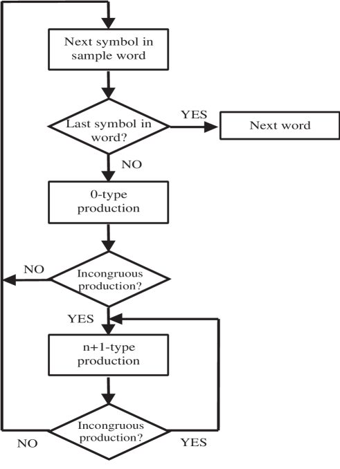
Unlike, for example, the rules for fuzzy logic inference, the structure of the formal language productions, obtained by our algorithm, is not established in advance. A mixture of different types of productions may be obtained in the grammar. This feature provides flexible adaptation in dynamical systems displaying distinct behavior in different regions of the working space.
In a controlled system the two types of variables, output variables and control variables, have a distinct nature. This is represented in our formalism by the assignment of terminal symbols to the dynamical variables and non-terminal symbols to the control. In turn, the productions represent the action of the control in the context of the past and present dynamics of the system. The languages generated in this way fall in the category of context-sensitive languages[12].
In practical applications the grammatical inference algorithm is completed with grammatical interpolation and a noise rejection mechanism. Grammatical interpolation is discussed in Section 3 and noise rejection is simply implemented by keeping only those productions that appear a sufficient number of times in the data. Also, for practical purposes, an upper bound is put on the order of the productions that the algorithm generates.
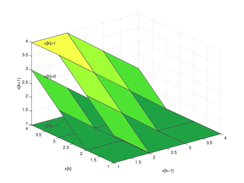
As a simple example, of how this methodology is used to model the dynamics, we consider the following piecewise linear system
| (12) |
The working domain of this dynamical systems is spanned by three distinct planes, depending on the values of the variable (Fig.2).
The assumed codification is
| 1 a | 1 A |
| 2 b | 0 B |
| 3 c | 1 C |
| 4 d |
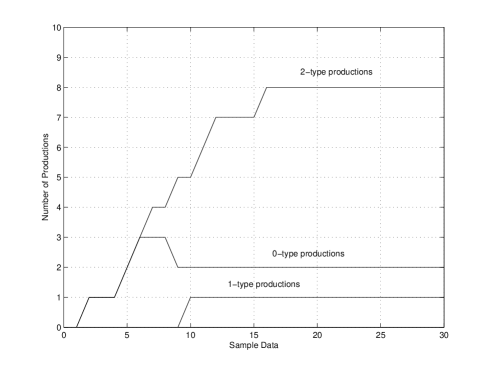
The language generated by this dynamical system is represented by a grammar , whose rewriting system has one type production, two type productions and twenty four type productions.
This system was used to test our on-line learning algorithm with a random input control signal . Fig.3 shows the evolution of the productions, extracted from randomly generated data, for the first 30 data points. One sees, for example, at the data point 19, the cancellation of a type production forced by a new type production. Also at data point 62 two contradictory type productions are discarded.
3 Modelling an electrical drive
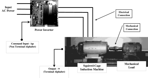
The linguistic coding described before has been used, in our laboratory, to model an experimental drive system, consisting of an electronically fed induction machine.
The experimental system is depicted in Fig.4. It is composed of an induction motor driven by a power inverter. Drive systems of this type are modelled using the electromechanical power conversion theory [19]. A 12-equations model represents the electrical drive system. The large number of variables hinders any attempt to perform on-line learning without huge computational costs. Therefore, one needs to simplify the electrical drive model.
Considering an input variable internal control loop [20], stator currents may be assumed to be controlled. The model is then reduced from a 12th to a 3rd order system [21] which, in the rotor flux reference frame, is
| (13) |
The rotor fluxes (,) and the rotor speed () are the state variables, and the stator current components (,) the control variables. is the rotor time constant, the mutual (stator-rotor) induction coefficient, the inertia coefficient, the rotor self-inductance coefficient, the friction coefficient and the load torque. With the reference frame rotor flux given by
| (14) |
one obtains from (13)
To obtain relevant training sets, two types of information, qualitative and quantitative, should be acquired. Qualitative information is obtained from the mathematical models. This leads to the choice of the relevant variables that describe the system behavior. This choice is very important to insure the existence of a functional relationship representative of the drive behavior[22]. Otherwise both learning and recognition would be impossible.
To obtain quantitative information experimental data is acquired. To obtain the data an excitation signal must be chosen. A possible approach would be to use a pseudo-random binary signal[23]. However, this signal is not the best choice for drive systems because it is filtered by mechanical time constants. It is better to use sinusoidal signals of different amplitudes and frequencies. In this way, frequencies and amplitudes may be adjusted within the limits of the drive response, thus avoiding the filtering problem and collecting data that adequately spans the operating domain.
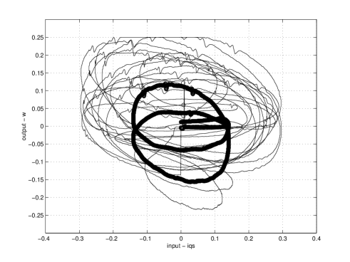
A grammar of the drive language is inferred from the (control) input - output experimental information. The current is kept constant, a non terminal alphabet is established from the quantification of the current and a terminal alphabet established from the output speed signal (). A representative training set is obtained with a sinusoidal reference signal containing a combination of different amplitudes and frequencies. Fig.5 shows the evolution, in the input/output space, of the training and test data sets, the test data being displayed in bold.
The acquisition of the training set is an essential step in obtaining a good knowledge of the system to be modelled. The training set must cover a representative part of the entire working domain.
3.1 Recognition results
To test the validity of the recognition process, two alphabets were considered. A quantification is established for both input and output variables, yielding a 60 symbol alphabet.
The inferred grammar contains 183 productions distributed in the following way: 5 type productions, 156 type productions and 22 type productions. To avoid the influence of noise on the inferred productions, a production is considered valid only if it appears more than a certain number of times, this parameter depending on the size the training set. This procedure works as a filter on noise perturbations.
Applying this grammar to the test set, we obtain the recognition results shown in Fig.6. The actual electromechanical drive speed is shown as a dotted line and the grammar response as a continuous one.
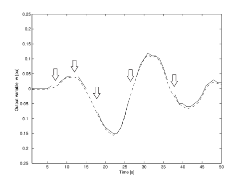
Apart from the quantification error, the recognition results may be considered satisfactory, because the evolution of the drive speed and the grammar results are similar. However, we must point out that there are some situations, indicated by the white arrows in Fig.6, where the grammar does not provide any answer. This happens when no production was inferred representing that particular input/output relationship. As explained later, a generalization method is used to establish non-learned productions.
For the second alphabet, a quantification interval ten times higher is assumed for both input and output variables, yielding now a 6-symbol alphabet, instead of the previous 60 symbols. The inferred grammar contains 36 productions, distributed in the following way: 0 type productions, 4 type productions and 32 type productions. Applying this grammar to the test set the recognition results are those shown in Fig.7. As before, the electromechanical drive speed is shown as a dotted line and the grammar response as a continuous one. The white arrows denote the absence of applicable productions.
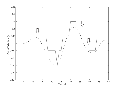
As expected, the quantitative modelling performance deteriorates, there being a larger difference between the measured drive speed and the grammatical reconstruction. However, if the important feature is the qualitative recognition of the drive speed, the results may still be considered as satisfactory. For a qualitative recognition process a limited alphabet is not a serious drawback. However, as in the larger grammar, the problem of non-existent productions is present here.
The discrete quantification performed within the grammatical inference algorithm implies a discrete response when recognition of the drive is performed. In order to improve the quantitative recognition capabilities of the algorithm two solutions may be used. The first is to increase the number of symbols in the alphabet to make a more accurate quantification. Alternatively one may use numerical interpolation of the productions. The first solution increases the number of productions thus slowing the recognition process. The second solution does not increase the number of productions.
To illustrate the operation of the interpolation process consider again the 60-symbol alphabet and another training set which is half the size of the one used for the results in Fig.6. After inferring the correspondent grammar, the recognition results are shown in Fig.8. It is seen that the recognition process has considerable faults because, for the reduced training set, the number of productions that is obtained is considerably smaller. A smaller training set led to a faulty grammar, which fails to recognize some words. However because the symbols in our alphabets are in correspondence with numerical values of the variables domain, a metric may be defined in the space of words. New productions may then be obtained, from those inferred from the smaller sample, by interpolation.
Grammatical interpolation establishes new productions by a structural matching procedure. The main idea of structural matching is based on a measure of similarity between the unknown input pattern and the available data structures. The measure of similarity is the distance between the non-existent production and the nearest productions. Several methods for structural word matching have been reported in the literature[24]. The basic algorithm states that the distance between two words is related to the sequence of edit operations (substitution, insertion, and deletion) required to transform one word into another. For any sequence of edit operations a cost function is considered
denotes the cost of a particular sequence , and the cost of a particular edit operation. The distance between two words and is defined as the minimum cost of transforming a word into another
When a word cannot be recognized because there is no production generating some symbol in that word, a grammatical interpolation formula is used to obtain the last terminal symbol in the right-hand side of the new production
This interpolation formula establishes a weighed average of the available productions of the required order, on an average distance between similar productions. The distance is the distance between the words in the left-hand side of the existent productions and the word of the new production.
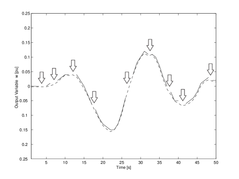
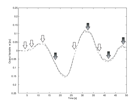
Fig.9 shows the recognition results for the same grammar as considered in Fig.8, when the grammatical interpolation procedure is applied. The effect of the non-existent productions is reduced, and the number of symbols that are not recognized much smaller. Grey arrows denote the interpolation of non-existent productions and white arrows productions that could not be obtained by interpolation.
By generalization we mean the ability of an algorithms to perform even under working conditions distinct of those observed during the learning phase. The interpolation process as described above provides generalization abilities to the algorithm. However this type of generalization is a local effect in the working space. For example, consider the training set shown in Fig.10.
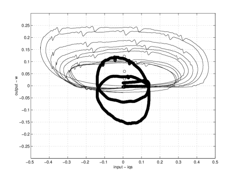
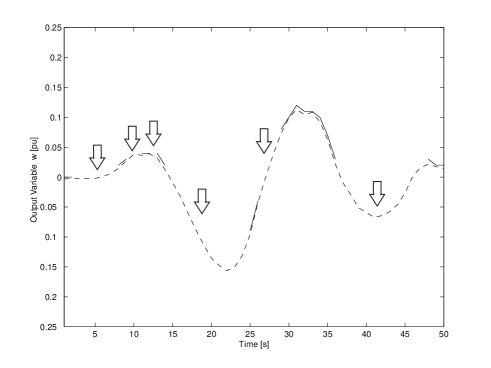
In this case the training set contains only positive speed values. Fig.11 shows the modelling results that are obtained using this sample data. Recognition fails for some of the domain areas not covered by the training data set. Namely symbols that code for negative drive speed are not recognized. Generalization has only a local effect. Therefore, experimental training data must always cover a significant part of the working domain.
4 Anomaly detection
Any grammar codes for the class of patterns that belong to the language the grammar generates. In this way one may use the grammar to recognize well formed strings and reject anomalous ones. Once one has learned the grammar of the strings generated by the system under normal conditions, if at a later time there is some fault in the dynamic system, strings that will be generated are not compatible with the learned grammar. It is also reasonable to assume that this might occur already at an early stage of the anomaly. The language algorithm might therefore be valuable as a tool for early fault detection.
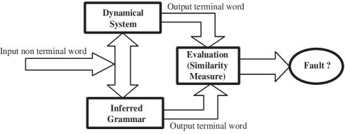
Detection of grammar anomalies is based on the same distance and similarity measures as considered before, for grammar interpolation. The anomaly detection algorithm (Fig.12) computes the distance between the string generated by the dynamical system and the one generated by the learned grammar. If this distance exceeds some threshold, a fault is reported.
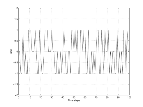
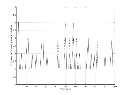
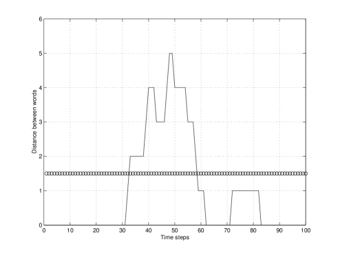
As a first example, let us consider the dynamical system represented by Eq.(12), with the same codification and inferred grammar as before. For the anomaly detection test we consider a random input during 100 time steps. A sustained anomaly was simulated between time steps 30 to 60, and a spurious one between time steps 80 to 85. The anomaly simulation is simply the replacement of the parameter 2 by 3 in Eq.(12). The dynamical system changes and therefore some of the strings that are generated do not match the learned grammar. Whenever the distance between the system-generated strings and those of the grammar exceeds a threshold, an anomaly is reported.
Figs.13-15 display the anomaly detection results. In response to the control variable both the learned grammar and the system produce terminal words. These are shown in Fig.14, the output of the grammar as a continuous line and the output of the dynamical system as a dashed line. They differ whenever there is an anomaly. Fig.15 displays the distance between words produced by the learned grammar and those of the dynamical system, for a word length of 10 symbols. This distance exceeds the threshold only for the sustained anomaly.
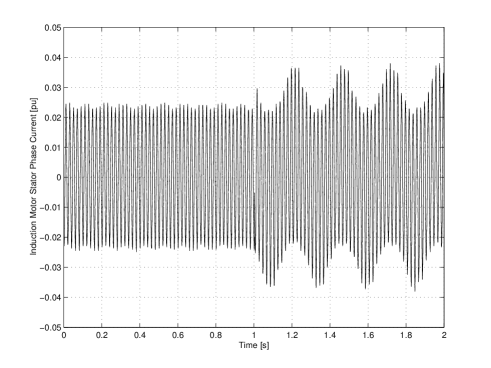
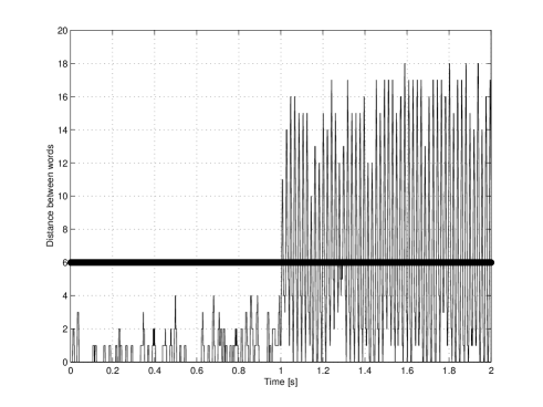
As a second example we consider anomaly detection in an induction motor. The anomaly is a rotor broken bar, and the variable coded as a terminal alphabet is the stator phase current. The learned grammar, representing the experimental drive system, is generated with the motor operating without anomaly. Fig16 shows the stator current deviation due to the presence of the anomaly between time 1 and 2 (seconds). Fig.17 shows the distance between the words generated by the learned grammar and those of the induction motor. Soon after the onset of the anomaly, this distance begins to exceed the threshold. A non-zero threshold must be defined because, as is seen in the figure, some deviations are obtained even without anomalies due to noise or even to small mismatches in the learned grammar.
5 Control
Once the grammar generated by a dynamical system is learned, this grammar, defining the structural features of the words produced by the linguistic source, is a model for the source. So it is possible to use the productions to predict the evolution of the system or to find the control string that leads from one state to another.
The basic idea of the control algorithm is as follows. A string of terminal symbols is given which represents the sequence of states that one wants the system to follow. Knowing the initial state of the system, for each symbol of the desired sequence of target states one chooses a production leading the system from its present state to the desired one. At each step the production that is chosen is the one that leads the system as close as possible to the desired state. The procedure is repeated until that symbol is reached and then one moves to the next target symbol.
As an example consider the dynamical system defined by Eq.(12). Suppose that the sequence of target states is ’’. Fig.18 shows the evolution of the system obtained by the control methodology described above. The target sequence is shown as a dashed line and the system evolution as a continuous line.
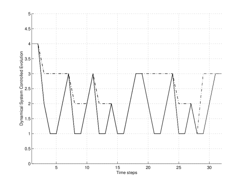
Notice that to evolve from one target symbol to another the system may have to pass through other terminal symbols. The control algorithm is robust in the sense that whenever, at some time , the expected evolution differs from the one predicted by the learned grammar, due to some perturbation or noise, it suffices to apply the same algorithm once more starting from the state at time .
6 Conclusions and Remarks
This paper proposes a characterization of controlled system dynamics by formal language techniques. The applications we have been concerned with are mostly electromechanical drives. However, the technique might also be useful for many other dynamical systems or industrial processes.
An important issue is the choice of an appropriate quantification for the feature space. This influences the choice and size of the alphabets and the dimension and complexity of the grammars. Also, good coverage of the working domain, in the learning stage, is essential to insure good generalization properties.
Unlike other approaches, the nature of the rules that define the dynamical system are not set up in advance, different types of productions being established on-line according to the incoming words from the linguist source. The method seems to provide good recognition results and a reasonable quantitative accuracy. Fuzzy logics approaches are probably more efficient when quantitative accuracy is very important and a good knowledge already exists concerning the rules of the system. However, if the dynamics is unknown or if pattern recognition is the important issue, the formal language approach seems quite promising.
Fault detection in control systems, industrial plants and power networks is a field where this work is being pursued and compared with immunity-based learning systems.
References
- [1] S. Wolfram; Computational theory of cellular automata, Commun. Math. Phys. 96 (1984) 15.
- [2] P. Grassberger; Toward a quantitative theory of self-generated complexity, Int. J. Theor. Phys. 25 (1986) 907.
- [3] J. P. Crutchfield and K. Young; Computation at the onset of chaos, in Complexity, Entropy and Physics of Information, SFI Studies in the Sciences of Complexity vol.8, W. H. Zurek (Ed.) pp. 223-267, 1990.
- [4] D. Auerbach and I. Procaccia; Grammatical complexity of strange sets, Phys. Rev. A41 (1990) 6602.
- [5] G. Troll; Formal languages in dynamical systems, chao-dyn/9305008, Acta Univ. Carolin. Math. Phys. 34 (1993) 117.
- [6] H. Xie; On formal languages in one-dimensional dynamical systems, Nonlinearity 6 (1993) 997.
- [7] Y. Wang and H. Xie; Grammatical complexity of unimodal maps with eventually periodic kneading sequences, Nonlinearity 7 (1994) 1419.
- [8] Collet, P. and Galves, A. and Lopes, A.; Maximum likelihood and minimum entropy identification of grammars, Random & Computational Dynamics, 3 (1995) 241.
- [9] P. Lakdawala; The computational complexity of symbolic dynamics at the onset of chaos, Phys. Rev. E53 (1996) 4477.
- [10] C. Moore; Dynamical recognizers: Real-time language recognition by analog computers, Santafe Institute working paper 96-05-023.
- [11] N. Chomsky; On certain formal properties of grammar, Information and Control 2 (1959) 137.
- [12] N. Chomsky; Aspects of the theory of syntax, MIT Press, Cambridge, Massachusetts, 1965.
- [13] R. N. Moll, M. A. Arbib and A. J. Kfoury; An introduction to formal language theory, Springer-Verlag, New York 1988.
- [14] G. Rozenberg and A. Salomaa; Handbook of formal languages, Springer-Verlag, Berlin 1997.
- [15] E. Mark Gold; Language identification in the limit, Information and Control 10 (1967) 447.
- [16] D. Angluin; Inductive inference of formal languages from positive data, Information and Control 45 (1980) 117.
- [17] K.S. Fu and T.L. Booth; Grammatical inference: Introduction and Survey Parts I and II”, IEEE Trans. on SMC 5, 1 (1975) 95 and IEEE Trans. on SMC 5, 4 (1975) 409.
- [18] Y. Sakakibara; Recent advances in grammatical inference, Theoretical Computer Science 185 (1997) 15-45.
- [19] A.E. Fitzgerald, C. Kingsley and S.D. Umans; Electric Machinery, 4th Edition, McGraw Hill, 1985.
- [20] J. F. Martins, A. J. Pires and J. F. Silva; A Novel and Simple Current Controller for Three-Phase PWM Power Inverters, IEEE Transactions on Industrial Electronics 45 (1998) 802
- [21] J. F. Martins, A. J. Pires and J. A.Dente, Automatic Input/Output Modeling of a Squirrel Cage Induction Motor Drive System using a Neural Network”; in Proc. of EPE97, pp. 4.632-4.637, Trondheim, Norway; September 1997.
- [22] J. F. Martins, A. J. Pires and J. A.Dente, A Choice of Variables in Automatic Modelling of AC Drive Systems, in Proc. of PEMC98, pp. 5.7- 5.12, Prague; Check Republic, Sept. 1998.
- [23] Teck-Seng Low, T.H. Lee and H.K. Lim, A methodology for neural network training from control of drives with nonlinearities, IEEE Trans. on Industrial Electronics 40 (1993) 243.
- [24] H. Bunke; String Matching for Structural Pattern Recognition, in Syntactic and Structural Pattern Recognition. Theory and Applications, H. Bunke and A. Sanfelui (Eds.), Series in Computer Science, World Scientific, Singapore 1990.