Also at   ]Center for Nonlinear Phenomena and Complex Systems, Universite Libre de Bruxelles, Code Postal 231, Campus Plaine, B-1050 Brussels, Belgium.

Fluctuation theorem for counting-statistics in electron transport through quantum junctions

Massimiliano Esposito [    Upendra Harbola    Shaul Mukamel Department of Chemistry, University of California, Irvine, California 92697, USA.
Abstract

We demonstrate that the probability distribution of the net number of electrons passing through a quantum system in a junction obeys a steady-state fluctuation theorem (FT) which can be tested experimentally by the full counting statistics (FCS) of electrons crossing the lead-system interface. The FCS is calculated using a many-body quantum master equation (QME) combined with a Liouville space generating function (GF) formalism. For a model of two coupled quantum dots, we show that the FT becomes valid for long binning times and provide an estimate for the finite-time deviations. We also demonstrate that the Mandel (or Fano) parameter associated with the incoming or outgoing electron transfers show subpoissonian (antibunching) statistics.

I Introduction

Various far-from-equilibrium relations, such as the Jarzynski relation Jarzynski1 ; Crooks99 ; Crooks00 or the fluctuation theorem (FT) Gallavotti ; Kurchan1 ; Lebowitz ; Searles ; Gaspard1 ; Seifert ; Broeck , obtained for classical systems during the past decade, provide new insights into the emergence of irreversible processes in physical systems Maesrev ; Gaspardrev . These relations follow from the observation that the ratio of the probability of a system forward and time-reversed trajectory is given by the exponential of a quantity, the trajectory entropy production, which when ensemble averaged, gives the entropy production in the system. These relations therefore quantify the probabilities of observing ”non-thermodynamic” trajectories with decreased trajectory entropy production. These probabilities are infinitesimally small in the macroscopic world but are non-negligible in microscopic systems. However, the ensemble averaged dynamics always satisfies the second law (entropy production always grows). With the recent progress in nano and mesoscopic sciences, these probabilities can now be measured Bustamente1 ; Bustamente2 . Because in the microscopic world quantum effects can be important, it is interesting to establish whether these fluctuation relations remain true in the quantum regime. This is still an open issue MukamelQJ ; STasaki ; Maes ; Monnai ; Allahverdyan ; Maes2 ; EspositoMukamel . One of the major obstacles for a general formulation of a quantum FT is the lack of a clear concept of a measurable trajectory. It is therefore helpful to consider systems undergoing a well-defined measurement process. In the counting statistics of photons emitted by an atom or a molecule driven out of equilibrium by a laser field Glauber ; Kelley ; Mandel ; Brown ; Mukamel03 ; Mukamel05 ; Mukamel06 ; BarkaiRev ; Orrit , a trajectory picture is provided by the history of the detected photons. However, the reverse trajectory (where the laser mode absorbs a photon from the molecule) is not easily measurable. Electron counting statistics provides on the other hand a clear trajectory picture given by the history of the electron transfers between the system and the leads, where the reverse trajectory (electron moving against the bias) is a measurable quantity. Electron counting statistics in nanosystems has attracted recent interest Levitov ; Buttiker ; Gurvitz ; Rammer1 ; Rammer2 ; Rammer3 ; Jauho ; Kießlich ; Utsumi ; Pederson ; Nazarov03 . Individual electrons crossing quantum dots have been measured Lu ; Fujisawa ; Bylander ; Gustavsson . Measuring the statistics of both forward and backward electron transfer events is essential to verify the FT and has recently been reported in Ref. Hirayama . Most studies have focused on the few lowest moments of the distribution. However, the FT is connected with the probabilities of large fluctuations which require the knowledge of the entire probability distribution.

In this paper, we use the many-electron QME derived in Ref. HarbolaEsposito and the generating operator (GO) formalism in Liouville space developed for photon counting statistics Glauber ; Kelley ; Mandel ; Brown ; Mukamel03 ; Mukamel05 ; Mukamel06 to calculate the FCS of electrons in biased quantum junctions. Our central formal result is an equation of motion for the GO whose solution can provide the full electron transfer probability distribution. Neglecting electron-electron interactions, this GO can be factorized into products of single orbital GO, each leading to a statistics similar to the one of the single resonant-level system studied in Ref. Nazarov03 . By constructing the current GO from the full electron counting GO, we show that the probability distribution of the net number of electrons k𝑘k entering the system from one of the system-lead interface [k(t)=1e0t𝑑τI(τ)𝑘𝑡1𝑒superscriptsubscript0𝑡differential-d𝜏𝐼𝜏k(t)=-\frac{1}{e}\int_{0}^{t}d\tau I(\tau), where I(τ)𝐼𝜏I(\tau) is the current and t𝑡t the measurement time also called binning time], satisfies: Pt(k)/Pt(k)=texp(βeVk)superscript𝑡subscript𝑃𝑡𝑘subscript𝑃𝑡𝑘𝛽𝑒𝑉𝑘P_{t}(k)/P_{t}(-k)\stackrel{{\scriptstyle t\to\infty}}{{=}}\exp{(\beta eVk)}, where eV𝑒𝑉eV is the difference between the left and right lead chemical potentials and β=(kbT)1𝛽superscriptsubscript𝑘𝑏𝑇1\beta=(k_{b}T)^{-1} the inverse temperature. The probability of observing a current in the direction favored by the bias voltage V𝑉V is exponentially larger than that of measuring the reverse current. For a non-biased junction the two currents are equiprobable.

The QME presented in section II is used to calculate the FCS of electrons in section III. In section IV, we define the GO for the net number of electron transfer and show that the FT holds for long measurement times. In section V we derive closed expressions for the current and its power spectrum and for the Mandel parameter. In section VI, we calculate the probability distribution for the net number of electron transfer for a model of two-coupled quantum dots and analyze the finite-time deviations to the FT. We also study the behavior of the average current and Mandel parameter as a function of the bias and temperature. Conclusions are drawn is section VII.

II The Quantum master equation

The quantum junction is made of a system (e.g. quantum dot or single molecule) coupled to two leads. The system Hamiltonian reads HS=sϵscscssubscript𝐻𝑆subscript𝑠subscriptitalic-ϵ𝑠superscriptsubscript𝑐𝑠subscript𝑐𝑠H_{S}=\sum_{s}\epsilon_{s}c_{s}^{\dagger}c_{s}, where cssuperscriptsubscript𝑐𝑠c_{s}^{\dagger} (cssubscript𝑐𝑠c_{s}) is the Fermi creation (annihilation) operator for the s𝑠s system orbital. The Hamiltonian of the left (right) lead is HL=lϵlclclsubscript𝐻𝐿subscript𝑙subscriptitalic-ϵ𝑙superscriptsubscript𝑐𝑙subscript𝑐𝑙H_{L}=\sum_{l}\epsilon_{l}c_{l}^{\dagger}c_{l} (HR=rϵrcrcrsubscript𝐻𝑅subscript𝑟subscriptitalic-ϵ𝑟superscriptsubscript𝑐𝑟subscript𝑐𝑟H_{R}=\sum_{r}\epsilon_{r}c_{r}^{\dagger}c_{r}), where l𝑙l (r𝑟r) runs over all the left (right) lead orbitals. The entire junction Hamiltonian is H=HS+HL+HR+HT𝐻subscript𝐻𝑆subscript𝐻𝐿subscript𝐻𝑅subscript𝐻𝑇H=H_{S}+H_{L}+H_{R}+H_{T} where HT=sν[Tsνcscν+h.c.]H_{T}=\sum_{s\nu}\left[T_{s\nu}c^{\dagger}_{s}c_{\nu}+h.c.\right] is the system-leads coupling (ν=l,r𝜈𝑙𝑟\nu=l,r). In HarbolaEsposito , we used second order perturbation theory in the lead-system interaction and projection operators in the number of electrons in the system to derive a QME describing the dynamics of the reduced system density matrix. The QME gives a Redfield equation Breuer in Fock space which only contains coherences between states with the same number of electrons. When the relaxation induced by the leads is much slower than the Bohr frequencies of the system, the fast oscillations in the interaction picture can be averaged out. This approximation, known as the rotating wave approximation (RWA) in quantum optics, is often performed on the Redfield equation to guarantee that the final QME is of the Lindblad form Breuer ; Gardiner ; Haake ; Spohn ; Tannoudji . Our QME finally reads

ρ˙nsuperscript˙𝜌𝑛\displaystyle\dot{\rho}^{n} =\displaystyle= i[HS,ρn]+s(vsscsρn+1cs+wsscsρn1csvsscscsρnwssρncscs+h.c.),\displaystyle-i[H_{S},\rho^{n}]+\sum_{s}\left(v_{ss}c_{s}\rho^{n+1}c_{s}^{\dagger}+w_{ss}c_{s}^{\dagger}\rho^{n-1}c_{s}-v_{ss}c_{s}^{\dagger}c_{s}\rho^{n}-w_{ss}\rho^{n}c_{s}c_{s}^{\dagger}+{\rm h.c.}\right)\;, (1)

where ρnsuperscript𝜌𝑛\rho^{n} is the reduced density matrix of the system projected into the n𝑛n electron part of the Fock space. The complete system density matrix is given by ρ=nρn𝜌subscript𝑛superscript𝜌𝑛\rho=\sum_{n}\rho^{n}. When summed over n𝑛n, Eq. (1) gives an equation for the total ρ𝜌\rho which is of the Lindblad form HarbolaEsposito . vsssubscript𝑣𝑠𝑠v_{ss}’s and wsssubscript𝑤𝑠𝑠w_{ss}’s are related to lead correlation functions. Assuming a quasi-continuous spectra for the leads and neglecting the level shift contributions (which only modify the bare Bohr frequencies of the system), we have

vssyvss(y);wssywss(y)\displaystyle v_{ss}\equiv\sum_{y}v_{ss}^{(y)}\ \ ;\ \ w_{ss}\equiv\sum_{y}w_{ss}^{(y)} (2)

where

vss(y)superscriptsubscript𝑣𝑠𝑠𝑦\displaystyle v_{ss}^{(y)} =\displaystyle= πny(ϵs)|Ts(y)(ϵs)|2(1fy(ϵs))𝜋subscript𝑛𝑦subscriptitalic-ϵ𝑠superscriptsuperscriptsubscript𝑇𝑠𝑦subscriptitalic-ϵ𝑠21subscript𝑓𝑦subscriptitalic-ϵ𝑠\displaystyle\pi n_{y}(\epsilon_{s})|T_{s}^{(y)}(\epsilon_{s})|^{2}(1-f_{y}(\epsilon_{s})) (3)
wss(y)superscriptsubscript𝑤𝑠𝑠𝑦\displaystyle w_{ss}^{(y)} =\displaystyle= πny(ϵs)|Ts(y)(ϵs)|2fy(ϵs).𝜋subscript𝑛𝑦subscriptitalic-ϵ𝑠superscriptsuperscriptsubscript𝑇𝑠𝑦subscriptitalic-ϵ𝑠2subscript𝑓𝑦subscriptitalic-ϵ𝑠\displaystyle\pi n_{y}(\epsilon_{s})|T_{s}^{(y)}(\epsilon_{s})|^{2}f_{y}(\epsilon_{s})\;.

ny(ϵ)subscript𝑛𝑦italic-ϵn_{y}(\epsilon) is the density of state of the left or right lead (y=L,R𝑦𝐿𝑅y=L,R) at energy ϵitalic-ϵ\epsilon. fy(ϵ)1/(exp[β(ϵμy)]+1)subscript𝑓𝑦italic-ϵ1𝛽italic-ϵsubscript𝜇𝑦1f_{y}(\epsilon)\equiv 1/(\exp{[\beta(\epsilon-\mu_{y})}]+1) denotes the Fermi distribution of the y𝑦y lead and μysubscript𝜇𝑦\mu_{y} is its chemical potentials. We assume μR=μ0subscript𝜇𝑅subscript𝜇0\mu_{R}=\mu_{0} and μL=μ0+eVsubscript𝜇𝐿subscript𝜇0𝑒𝑉\mu_{L}=\mu_{0}+eV, where V𝑉V is the bias [see Fig.1]. wss(y)superscriptsubscript𝑤𝑠𝑠𝑦w_{ss}^{(y)} is the electron transfer rate from lead y𝑦y to the s𝑠s orbital and vss(y)superscriptsubscript𝑣𝑠𝑠𝑦v_{ss}^{(y)} is the rate for the reverse process. These obey the relation

vss(y)=eβ(ϵsμy)wss(y),superscriptsubscript𝑣𝑠𝑠𝑦superscript𝑒𝛽subscriptitalic-ϵ𝑠subscript𝜇𝑦superscriptsubscript𝑤𝑠𝑠𝑦\displaystyle v_{ss}^{(y)}=e^{\beta(\epsilon_{s}-\mu_{y})}w_{ss}^{(y)}\;, (4)

so that

vss(R)wss(L)vss(L)wss(R)=eβeV.superscriptsubscript𝑣𝑠𝑠𝑅superscriptsubscript𝑤𝑠𝑠𝐿superscriptsubscript𝑣𝑠𝑠𝐿superscriptsubscript𝑤𝑠𝑠𝑅superscript𝑒𝛽𝑒𝑉\displaystyle\frac{v_{ss}^{(R)}w_{ss}^{(L)}}{v_{ss}^{(L)}w_{ss}^{(R)}}=e^{\beta eV}\;. (5)

III Generating-function for electron-counting statistics

We consider a system with M𝑀M orbitals and n𝑛n spinless electrons, so that n=0,1,,M𝑛01𝑀n=0,1,\ldots,M. The number of n𝑛n-electron many-body states (hereafter denoted states) is given by CnM=M!(Mn)!n!subscriptsuperscript𝐶𝑀𝑛𝑀𝑀𝑛𝑛C^{M}_{n}=\frac{M!}{(M-n)!n!}. The total number of Fock space states is Ntot=n=0MCnM=2Msubscript𝑁totsuperscriptsubscript𝑛0𝑀subscriptsuperscript𝐶𝑀𝑛superscript2𝑀N_{\rm tot}=\sum_{n=0}^{M}C^{M}_{n}=2^{M}. As a result of the weak lead-system coupling and infinite leads assumption, the Fock space coherences (FSC) between many-body states with different n𝑛n are neglected and the number of elements of the full many-body density matrix reduces from Ntot2=4Msuperscriptsubscript𝑁tot2superscript4𝑀N_{\rm tot}^{2}=4^{M} to Nred2=n=0M(CnM)2superscriptsubscript𝑁red2superscriptsubscript𝑛0𝑀superscriptsubscriptsuperscript𝐶𝑀𝑛2N_{\rm red}^{2}=\sum_{n=0}^{M}(C^{M}_{n})^{2}. The space of the density matrices where FSC have been eliminated constitute our reduced Liouville space. By expanding the QME (1) in the eigenbasis of the system, the population dynamics obeys a birth and death master equation which is decoupled from the coherence dynamics. Electron-transfer events are counted by identifying the terms in the QME which are responsible for the transitions between the populations. Their sequence constitutes a ”trajectory”.

We shall recast the QME (1) in our reduced Liouville space as

|ρ˙=(^+γ^+Γ^)|ρ^|ρ.\displaystyle|\dot{\rho}\gg=\big{(}\hat{{\cal L}}+\hat{\gamma}+\hat{\Gamma}\big{)}|\rho\gg\equiv\hat{{\cal M}}|\rho\gg\;. (6)

^^\hat{{\cal M}} is the generator of the QME. ^^\hat{{\cal L}} describes the isolated system dynamics

^^\displaystyle\hat{{\cal L}} =\displaystyle= isϵs[cscs,].𝑖subscript𝑠subscriptitalic-ϵ𝑠superscriptsubscript𝑐𝑠subscript𝑐𝑠\displaystyle-i\sum_{s}\epsilon_{s}[c_{s}^{\dagger}c_{s},\cdot]\;. (7)

We denote the four possible processes depicted in Fig. 1 by η=1,2,3,4𝜂1234\eta=1,2,3,4. η=1𝜂1\eta=1 and η=3𝜂3\eta=3 represent electron transfer from the system to the left and right lead whereas η=2𝜂2\eta=2 and η=4𝜂4\eta=4 represent the electron transfer from the left and right lead to the system. The orbital through which electron transfer occurs is denoted by s𝑠s. Γ^^Γ\hat{\Gamma} is responsible for electron transfers and is made of the non-diagonal terms of the generator which couple the populations

Γ^^Γ\displaystyle\hat{\Gamma} =\displaystyle= νΓ^ν,subscript𝜈subscript^Γ𝜈\displaystyle\sum_{\nu}\hat{\Gamma}_{\nu}\;, (8)

where ν=(η,s)𝜈𝜂𝑠\nu=(\eta,s), ν=η=14s=1Msubscript𝜈superscriptsubscript𝜂14superscriptsubscript𝑠1𝑀\sum_{\nu}=\sum_{\eta=1}^{4}\sum_{s=1}^{M}, and

Γ^(1,s)subscript^Γ1𝑠\displaystyle\hat{\Gamma}_{(1,s)} \displaystyle\equiv 2vss(L)cscs;Γ^(2,s)2wss(L)cscs\displaystyle 2v_{ss}^{(L)}c_{s}\cdot c_{s}^{\dagger}\ \ ;\ \ \hat{\Gamma}_{(2,s)}\equiv 2w_{ss}^{(L)}c_{s}^{\dagger}\cdot c_{s}
Γ^(3,s)subscript^Γ3𝑠\displaystyle\hat{\Gamma}_{(3,s)} \displaystyle\equiv 2vss(R)cscs;Γ^(4,s)2wss(R)cscs.\displaystyle 2v_{ss}^{(R)}c_{s}\cdot c_{s}^{\dagger}\ \ ;\ \ \hat{\Gamma}_{(4,s)}\equiv 2w_{ss}^{(R)}c_{s}^{\dagger}\cdot c_{s}\>. (9)

γ^^𝛾\hat{\gamma} describes the diagonal terms of the generator

γ^^𝛾\displaystyle\hat{\gamma} =\displaystyle= νγ^ν.subscript𝜈subscript^𝛾𝜈\displaystyle\sum_{\nu}\hat{\gamma}_{\nu}\;. (10)

In analogy to Γ^^Γ\hat{\Gamma}, we identify the various contributions to γ^^𝛾\hat{\gamma} from the different active orbitals

γ^(1,s)subscript^𝛾1𝑠\displaystyle\hat{\gamma}_{(1,s)} \displaystyle\equiv vss(L)[cscs,]+;γ^(2,s)wss(L)[cscs,]+\displaystyle-v_{ss}^{(L)}[c_{s}^{\dagger}c_{s},\cdot]_{+}\ \ ;\ \ \hat{\gamma}_{(2,s)}\equiv w_{ss}^{(L)}[c_{s}c_{s}^{\dagger},\cdot]_{+}
γ^(3,s)subscript^𝛾3𝑠\displaystyle\hat{\gamma}_{(3,s)} \displaystyle\equiv vss(R)[cscs,]+;γ^(4,s)wss(R)[cscs,]+.\displaystyle-v_{ss}^{(R)}[c_{s}^{\dagger}c_{s},\cdot]_{+}\ \ ;\ \ \hat{\gamma}_{(4,s)}\equiv w_{ss}^{(R)}[c_{s}c_{s}^{\dagger},\cdot]_{+}\;. (11)

We can now calculate the full electron counting statistics using the formalism developed for photon counting statistics Glauber ; Kelley ; Mandel ; Brown ; Mukamel03 ; Mukamel05 ; Mukamel06 ; BarkaiRev ; Orrit . Starting with a trajectory picture of the QME evolution in terms of electron transfer histories, we shall calculate the probabilities of these trajectories and their associated generating function (GF).
The system density matrix conditional to measuring 𝕜𝕜\mathbb{k} electron transfers during an interval of time t𝑡t is denoted ρ(𝕜)(t)superscript𝜌𝕜𝑡\rho^{(\mathbb{k})}(t). We use the compact notation defined in appendix A [see (53)]. 𝕜𝕜\mathbb{k} is a vector with components kνsubscript𝑘𝜈k_{\nu}. The probability to measure 𝕜𝕜\mathbb{k} electron transfers during a time interval t𝑡t is obtained by tracing the conditional system density matrix

P(t,𝕜)=I|ρ(𝕜)(t).\displaystyle P(t,\mathbb{k})=\ll I|\rho^{(\mathbb{k})}(t)\gg\;. (12)

The trace of an Hilbert space operator A𝐴A, TrATr𝐴{\rm Tr}A, is denoted as a scalar product in Liouville space I|Amuch-less-thanabsentconditional𝐼𝐴much-greater-thanabsent\ll I|A\gg, where I𝐼I is the unity operator.

The generating function (GF) associated with this probability distribution is defined as

G(t,𝝀)𝐺𝑡𝝀\displaystyle G(t,\bm{\lambda}) \displaystyle\equiv 𝕜P(t,𝕜)e𝝀𝕜,subscript𝕜𝑃𝑡𝕜superscript𝑒𝝀𝕜\displaystyle\sum_{\mathbb{k}}P(t,\mathbb{k})e^{\bm{\lambda}\cdot\mathbb{k}}\;, (13)

where 𝝀𝕜=νλνkν𝝀𝕜subscript𝜈subscript𝜆𝜈subscript𝑘𝜈\bm{\lambda}\cdot\mathbb{k}=\sum_{\nu}\lambda_{\nu}k_{\nu}. Similarly, we define the generating operator (GO) as

|G(t,𝝀)\displaystyle|G(t,\bm{\lambda})\gg \displaystyle\equiv 𝕜|ρ(𝕜)(t)e𝝀𝕜.much-greater-thanconditionalsubscript𝕜superscript𝜌𝕜𝑡superscript𝑒𝝀𝕜\displaystyle\sum_{\mathbb{k}}|\rho^{(\mathbb{k})}(t)\gg e^{\bm{\lambda}\cdot\mathbb{k}}\;. (14)

The GF is obtained by tracing the GO

G(t,𝝀)=I|G(t,𝝀).\displaystyle G(t,\bm{\lambda})=\ll I|G(t,\bm{\lambda})\gg\;. (15)

An evolution equation for the GO is derived in appendix A starting with the QME

|G˙(t,𝝀)=𝒲^(𝝀)|G(t,𝝀),\displaystyle|\dot{G}(t,\bm{\lambda})\gg=\hat{{\cal W}}(\bm{\lambda})|G(t,\bm{\lambda})\gg\;, (16)

where

𝒲^(𝝀)=^+ν(eλν1)Γ^ν^𝒲𝝀^subscript𝜈superscript𝑒subscript𝜆𝜈1subscript^Γ𝜈\displaystyle\hat{{\cal W}}(\bm{\lambda})=\hat{{\cal M}}+\sum_{\nu}(e^{\lambda_{\nu}}-1)\hat{\Gamma}_{\nu} (17)

is the generator of the GO evolution equation. Using the initial condition |G(0;𝝀)=|ρ(0)|G(0;\bm{\lambda})\gg=|\rho(0)\gg, the solution of (16), given in appendix B, provides the GF at all times

G(t,𝝀)=I|e𝒲^(𝝀)t|ρ(0).\displaystyle G(t,\bm{\lambda})=\ll I|e^{\hat{{\cal W}}(\bm{\lambda})t}|\rho(0)\gg\;. (18)

The GF contains the entire information about the electron counting statistics. The probability distribution is obtained by inverting Eq. (13)

P(t,𝕜)=02π𝑑𝝀G(t,i𝝀)ei𝝀𝕜.𝑃𝑡𝕜superscriptsubscript02𝜋differential-d𝝀𝐺𝑡𝑖𝝀superscript𝑒𝑖𝝀𝕜\displaystyle P(t,\mathbb{k})=\int_{0}^{2\pi}d\bm{\lambda}\;G(t,i\bm{\lambda})e^{-i\bm{\lambda}\cdot\mathbb{k}}\;. (19)

Moments of the distribution are given by derivatives of the GF

n1λν1n1n2λν2n2nNλνNnNG(t,𝝀)|𝝀=0=kν1n1kν2n2kνNnNt.evaluated-atsuperscriptsubscript𝑛1superscriptsubscript𝜆subscript𝜈1subscript𝑛1superscriptsubscript𝑛2superscriptsubscript𝜆subscript𝜈2subscript𝑛2superscriptsubscript𝑛𝑁superscriptsubscript𝜆subscript𝜈𝑁subscript𝑛𝑁𝐺𝑡𝝀𝝀0subscriptdelimited-⟨⟩superscriptsubscript𝑘subscript𝜈1subscript𝑛1superscriptsubscript𝑘subscript𝜈2subscript𝑛2superscriptsubscript𝑘subscript𝜈𝑁subscript𝑛𝑁𝑡\displaystyle\left.\frac{\partial^{n_{1}}}{\partial\lambda_{\nu_{1}}^{n_{1}}}\frac{\partial^{n_{2}}}{\partial\lambda_{\nu_{2}}^{n_{2}}}\cdots\frac{\partial^{n_{N}}}{\partial\lambda_{\nu_{N}}^{n_{N}}}G(t,\bm{\lambda})\right|_{\bm{\lambda}=0}=\langle k_{\nu_{1}}^{n_{1}}k_{\nu_{2}}^{n_{2}}\cdots k_{\nu_{N}}^{n_{N}}\rangle_{t}\;. (20)

We also define

S(𝝀)limt1tlnG(t,𝝀).𝑆𝝀subscript𝑡1𝑡𝐺𝑡𝝀\displaystyle S(\bm{\lambda})\equiv-\lim_{t\to\infty}\frac{1}{t}\ln G(t,\bm{\lambda})\;. (21)

This will be useful to calculate the statistical properties of steady-state currents.

IV Fluctuation theorem for the net number of electrons transferred

We will now focus on the statistical properties of the charge currents across the junction. We adopt the standard convention that the direction of the charge current is opposite to the electron transfers [see Fig.(1)]. The number of electrons transferred via process η𝜂\eta through orbital s𝑠s during a time interval t𝑡t is given by

kν(t)=1e0t𝑑τIν(τ),subscript𝑘𝜈𝑡1𝑒superscriptsubscript0𝑡differential-d𝜏subscript𝐼𝜈𝜏\displaystyle k_{\nu}(t)=-\frac{1}{e}\int_{0}^{t}d\tau I_{\nu}(\tau)\;, (22)

where Iν(τ)subscript𝐼𝜈𝜏I_{\nu}(\tau) is the corresponding charge current [ν=(η,s)𝜈𝜂𝑠\nu=(\eta,s)]. The net number of electron transfer events between the left (right) lead-system interface, through orbital s𝑠s, during time t𝑡t is

k(L,s)(t)k(2,s)(t)k(1,s)(t)=1e0tdτI(L,s)(τ),k(R,s)(t)k(3,s)(t)k(4,s)(t)=1e0tdτI(R,s)(τ).\displaystyle k_{(L,s)}(t)\equiv k_{(2,s)}(t)-k_{(1,s)}(t)=-\frac{1}{e}\int_{0}^{t}d\tau I_{(L,s)}(\tau)\ \ \;,\ \ k_{(R,s)}(t)\equiv k_{(3,s)}(t)-k_{(4,s)}(t)=-\frac{1}{e}\int_{0}^{t}d\tau I_{(R,s)}(\tau)\;. (23)

where the charge current at the left [right] lead-system interface passing through the s𝑠s’th system orbital is given by I(L,s)(t)I(2,s)(t)I(1,s)(t)subscript𝐼𝐿𝑠𝑡subscript𝐼2𝑠𝑡subscript𝐼1𝑠𝑡I_{(L,s)}(t)\equiv I_{(2,s)}(t)-I_{(1,s)}(t) [I(R,s)(t)I(3,s)(t)I(4,s)(t)subscript𝐼𝑅𝑠𝑡subscript𝐼3𝑠𝑡subscript𝐼4𝑠𝑡I_{(R,s)}(t)\equiv I_{(3,s)}(t)-I_{(4,s)}(t)]. The GF associated with the left and right net number of electron transfer G(t,𝝀L,𝝀R)𝐺𝑡subscript𝝀𝐿subscript𝝀𝑅G(t,\bm{\lambda}_{L},\bm{\lambda}_{R}) is the GF of the FCS G(t,𝝀)𝐺𝑡𝝀G(t,\bm{\lambda}) where λ1,s=λ2,sλL,ssubscript𝜆1𝑠subscript𝜆2𝑠subscript𝜆𝐿𝑠\lambda_{1,s}=-\lambda_{2,s}\equiv\lambda_{L,s} and λ4,s=λ3,sλR,ssubscript𝜆4𝑠subscript𝜆3𝑠subscript𝜆𝑅𝑠\lambda_{4,s}=-\lambda_{3,s}\equiv\lambda_{R,s}. Defining the vectors 𝝀Lsubscript𝝀𝐿\bm{\lambda}_{L} (𝝀Rsubscript𝝀𝑅\bm{\lambda}_{R}) with components λL,ssubscript𝜆𝐿𝑠\lambda_{L,s} (λR,ssubscript𝜆𝑅𝑠\lambda_{R,s}), we have

G(t,𝝀L,𝝀R)𝐺𝑡subscript𝝀𝐿subscript𝝀𝑅\displaystyle G(t,\bm{\lambda}_{L},\bm{\lambda}_{R}) =\displaystyle= 𝝀L,𝝀RP(t,𝕜L,𝕜R)e𝝀L𝕜Le𝝀R𝕜R.subscriptsubscript𝝀𝐿subscript𝝀𝑅𝑃𝑡subscript𝕜𝐿subscript𝕜𝑅superscript𝑒subscript𝝀𝐿subscript𝕜𝐿superscript𝑒subscript𝝀𝑅subscript𝕜𝑅\displaystyle\sum_{\bm{\lambda}_{L},\bm{\lambda}_{R}}P(t,\mathbb{k}_{L},\mathbb{k}_{R})e^{-\bm{\lambda}_{L}\cdot\mathbb{k}_{L}}e^{-\bm{\lambda}_{R}\cdot\mathbb{k}_{R}}\;. (24)

For clarity, we hereafter consider the left GF. The right one may be calculated similarly. The GF for the left net number of electron transfer G(t,𝝀L)𝐺𝑡subscript𝝀𝐿G(t,\bm{\lambda}_{L}) is defined from (24) by taking 𝝀R=0subscript𝝀𝑅0\bm{\lambda}_{R}=0. Using Eq. (81), we find that the generator 𝒲^s(λ(L,s))subscript^𝒲𝑠subscript𝜆𝐿𝑠\hat{{\cal W}}_{s}(\lambda_{(L,s)}) of the evolution of the single orbital GF Gs(t,λ(L,s))subscript𝐺𝑠𝑡subscript𝜆𝐿𝑠G_{s}(t,\lambda_{(L,s)}) for the net number of electron transfer, via the single orbital s𝑠s, through the left lead-system interface is given by

Gs(t,λ(L,s))subscript𝐺𝑠𝑡subscript𝜆𝐿𝑠\displaystyle G_{s}(t,\lambda_{(L,s)}) =\displaystyle= c+(0)eg+(λ(L,s))t(g1;1+(λ(L,s))+g0;0+(λ(L,s)))subscript𝑐0superscript𝑒subscript𝑔subscript𝜆𝐿𝑠𝑡subscriptsuperscript𝑔11subscript𝜆𝐿𝑠subscriptsuperscript𝑔00subscript𝜆𝐿𝑠\displaystyle c_{+}(0)e^{g_{+}(\lambda_{(L,s)})t}\big{(}g^{+}_{1;1}(\lambda_{(L,s)})+g^{+}_{0;0}(\lambda_{(L,s)})\big{)} (25)
+c(0)eg(λ(L,s))t(g1;1(λ(L,s))+g0;0(λ(L,s))),subscript𝑐0superscript𝑒subscript𝑔subscript𝜆𝐿𝑠𝑡subscriptsuperscript𝑔11subscript𝜆𝐿𝑠subscriptsuperscript𝑔00subscript𝜆𝐿𝑠\displaystyle+c_{-}(0)e^{g_{-}(\lambda_{(L,s)})t}\big{(}g^{-}_{1;1}(\lambda_{(L,s)})+g^{-}_{0;0}(\lambda_{(L,s)})\big{)}\;,

where, using (80) and (5), the eigenvalues of the generator are given by

g±(λ(L,s))subscript𝑔plus-or-minussubscript𝜆𝐿𝑠\displaystyle g_{\pm}(\lambda_{(L,s)}) =\displaystyle= (vss+wss2)±(vss+wss2)2+vss(R)wss(L)[eβeV(eλ(L,s)1)+(eλ(L,s)1)].plus-or-minussubscript𝑣𝑠𝑠subscript𝑤𝑠𝑠2superscriptsubscript𝑣𝑠𝑠subscript𝑤𝑠𝑠22superscriptsubscript𝑣𝑠𝑠𝑅superscriptsubscript𝑤𝑠𝑠𝐿delimited-[]superscript𝑒𝛽𝑒𝑉superscript𝑒subscript𝜆𝐿𝑠1superscript𝑒subscript𝜆𝐿𝑠1\displaystyle-\left(\frac{v_{ss}+w_{ss}}{2}\right)\pm\sqrt{\left(\frac{v_{ss}+w_{ss}}{2}\right)^{2}+v_{ss}^{(R)}w_{ss}^{(L)}\left[e^{-\beta eV}(e^{\lambda_{(L,s)}}-1)+(e^{-\lambda_{(L,s)}}-1)\right]}\;. (26)

These possess the symmetry g(λ(L,s))=g(βeVλ(L,s))𝑔subscript𝜆𝐿𝑠𝑔𝛽𝑒𝑉subscript𝜆𝐿𝑠g(\lambda_{(L,s)})=g(\beta eV-\lambda_{(L,s)}) so that, using Ss(λ(L,s))limt1tlnGs(t,λ(L,s))subscript𝑆𝑠subscript𝜆𝐿𝑠subscript𝑡1𝑡subscript𝐺𝑠𝑡subscript𝜆𝐿𝑠S_{s}(\lambda_{(L,s)})\equiv-\lim_{t\to\infty}\frac{1}{t}\ln G_{s}(t,\lambda_{(L,s)}) and (25),

Ss(λ(L,s))=Ss(βeVλ(L,s)).subscript𝑆𝑠subscript𝜆𝐿𝑠subscript𝑆𝑠𝛽𝑒𝑉subscript𝜆𝐿𝑠\displaystyle S_{s}(\lambda_{(L,s)})=S_{s}(\beta eV-\lambda_{(L,s)})\;. (27)

In appendix B, we show that the many-body GF can be factorized into a product of single orbital GF [see (82)]. The GF for the total current (irrespective of the carrying orbitals) by setting λ(L,s)=λLsubscript𝜆𝐿𝑠subscript𝜆𝐿\lambda_{(L,s)}=\lambda_{L} in 𝝀Lsubscript𝝀𝐿\bm{\lambda}_{L}) can therefore be written

G(t,λL)=mMegm(λL)tI|gm(λL)g~m(λL)|ρ(0),\displaystyle G(t,\lambda_{L})=\sum_{m}^{M}e^{g_{m}(\lambda_{L})t}\ll I|g_{m}(\lambda_{L})\gg\ll\tilde{g}_{m}(\lambda_{L})|\rho(0)\gg\;, (28)

where gm(λL)subscript𝑔𝑚subscript𝜆𝐿g_{m}(\lambda_{L}), |gm(λL)|g_{m}(\lambda_{L})\gg and g~m(λL)|\ll\tilde{g}_{m}(\lambda_{L})| are respectively the many-body eigenvalues, the right and the left eigenvector of the generator. Since the many-body eigenvalues corresponding to populations are made of 2Msuperscript2𝑀2^{M} possible sums of single-body orbital eigenvalues (26), they also satisfy the symmetry g(λL)=g(βeVλL)𝑔subscript𝜆𝐿𝑔𝛽𝑒𝑉subscript𝜆𝐿g(\lambda_{L})=g(\beta eV-\lambda_{L}) so that, using (21),

S(λL)=S(βeVλL).𝑆subscript𝜆𝐿𝑆𝛽𝑒𝑉subscript𝜆𝐿\displaystyle S(\lambda_{L})=S(\beta eV-\lambda_{L})\;. (29)

An important point is that the eigenvalues of the generator associated with the right GF are the same as those of the left GF so that S(λL)=S(λR)𝑆subscript𝜆𝐿𝑆subscript𝜆𝑅S(\lambda_{L})=S(\lambda_{R}). The eigenvectors will however be different and G(t,λL)G(t,λR)𝐺𝑡subscript𝜆𝐿𝐺𝑡subscript𝜆𝑅G(t,\lambda_{L})\neq G(t,\lambda_{R}). This means that, in general, the electron transfer statistics at the left and right interface of the junction can be different. However, the statistical properties which can be obtained from S(λ)𝑆𝜆S(\lambda) are the same on the two interface. We will see that these include for example the FT [which follows from (29)], the steady state average current [see (95)], the current power spectrum at zero frequency [see (98)] or the asymptotic value of the Mandel parameter [see (101)]. Hereafter, we therefore omit the L,R𝐿𝑅L,R labeling in the corresponding quantities.

In appendix C, we use the theory of large deviations to show that the symmetry (29) implies at long times

P(t,k)P(t,k)=teβeVk.superscript𝑡𝑃𝑡𝑘𝑃𝑡𝑘superscript𝑒𝛽𝑒𝑉𝑘\displaystyle\frac{P(t,k)}{P(t,-k)}\stackrel{{\scriptstyle t\to\infty}}{{=}}e^{\beta eVk}\;. (30)

This is the FT for the net number of electrons k𝑘k crossing the junction at each system-lead interface. Using (27), we note that the FT also holds for the net number of charges which passed through each orbital k(y,s)subscript𝑘𝑦𝑠k_{(y,s)} (y=L,R𝑦𝐿𝑅y=L,R). A similar result was pointed out in Ref. GaspardAndrieux2 for a single resonant level in the large Coulomb repulsion limit excluding double occupancy. The FT implies that measuring electron transfers in the direction favored by the bias is exponentially more probable than the reverse process. The argument of the exponential is proportional to the nonequilibrium constrains of the junction βeV𝛽𝑒𝑉\beta eV so that at equilibrium (V=0𝑉0V=0) the two probabilities are identical.

V Average current, Mandel parameter and power spectrum

In appendix D, we show how currents, moments and cumulants can be obtained from the GF. Using these results and the expressions for the eigenvalue with the smallest absolute value of the GF generators (80), we derive closed expressions for the steady state currents, their zero frequency power spectrum and the asymptotic value of the Mandel parameter.

Using (95) and (80), the four steady state average currents through orbital s𝑠s are given by

I(1,s)stsubscriptdelimited-⟨⟩subscript𝐼1𝑠st\displaystyle\langle I_{(1,s)}\rangle_{\rm st} =\displaystyle= 2evss(L)wssvss+wss,I(2,s)st=2ewss(L)vssvss+wss\displaystyle-2ev_{ss}^{(L)}\frac{w_{ss}}{v_{ss}+w_{ss}}\;\ \ \;,\ \ \;\langle I_{(2,s)}\rangle_{\rm st}=-2ew_{ss}^{(L)}\frac{v_{ss}}{v_{ss}+w_{ss}}
I(3,s)stsubscriptdelimited-⟨⟩subscript𝐼3𝑠st\displaystyle\langle I_{(3,s)}\rangle_{\rm st} =\displaystyle= 2evss(R)wssvss+wss,I(4,s)st=2ewss(R)vssvss+wss.\displaystyle-2ev_{ss}^{(R)}\frac{w_{ss}}{v_{ss}+w_{ss}}\;\ \ \;,\ \ \;\langle I_{(4,s)}\rangle_{\rm st}=-2ew_{ss}^{(R)}\frac{v_{ss}}{v_{ss}+w_{ss}}\;. (31)

The total current associated with the process η𝜂\eta is obtained by summing over the orbitals Iηst=sMI(η,s)stsubscriptdelimited-⟨⟩subscript𝐼𝜂stsuperscriptsubscript𝑠𝑀subscriptdelimited-⟨⟩subscript𝐼𝜂𝑠st\langle I_{\eta}\rangle_{\rm st}=\sum_{s}^{M}\langle I_{(\eta,s)}\rangle_{\rm st}. The Fano parameter Fν(t)subscript𝐹𝜈𝑡F_{\nu}(t) and the closely related Mandel parameter Mν(t)subscript𝑀𝜈𝑡M_{\nu}(t) of each of these processes ν=(η,s)𝜈𝜂𝑠\nu=(\eta,s) are defined as

Fν(t)Mν(t)+1kν2kνt2kνt.subscript𝐹𝜈𝑡subscript𝑀𝜈𝑡1delimited-⟨⟩superscriptsubscript𝑘𝜈2superscriptsubscriptdelimited-⟨⟩subscript𝑘𝜈𝑡2subscriptdelimited-⟨⟩subscript𝑘𝜈𝑡\displaystyle F_{\nu}(t)\equiv M_{\nu}(t)+1\equiv\frac{\langle k_{\nu}^{2}\rangle-\langle k_{\nu}\rangle_{t}^{2}}{\langle k_{\nu}\rangle_{t}}\;. (32)

The Mandel parameter vanishes for a Poisson process. M<0𝑀0M<0 (M>0𝑀0M>0) implies subpoissonian (superpoissonian) statistics. At steady state, using (100), we find

Mν()=1eIνstvss+wss.subscript𝑀𝜈1𝑒subscriptdelimited-⟨⟩subscript𝐼𝜈stsubscript𝑣𝑠𝑠subscript𝑤𝑠𝑠\displaystyle M_{\nu}(\infty)=\frac{1}{e}\frac{\langle I_{\nu}\rangle_{\rm st}}{v_{ss}+w_{ss}}\;. (33)

Another quantity of interest is the zero frequency power spectrum of the current Aννsubscript𝐴𝜈𝜈A_{\nu\nu} associated with the processes ν𝜈\nu [see Eq. (98)]. Mν(t)subscript𝑀𝜈𝑡M_{\nu}(t) and Fν(t)subscript𝐹𝜈𝑡F_{\nu}(t) are easily related to it by Aνν=eIνstFν()subscript𝐴𝜈𝜈𝑒subscriptdelimited-⟨⟩subscript𝐼𝜈stsubscript𝐹𝜈A_{\nu\nu}=e\langle I_{\nu}\rangle_{\rm st}F_{\nu}(\infty). The zero frequency power spectrum for the total current associated with the process η𝜂\eta is given by Aη=sMAννsubscript𝐴𝜂superscriptsubscript𝑠𝑀subscript𝐴𝜈𝜈A_{\eta}=\sum_{s}^{M}A_{\nu\nu}. The Mandel or Fano parameters cannot be expressed as such an orbital sum. It is therefore convenient to calculate them from Sηsubscript𝑆𝜂S_{\eta} and Iηstsubscriptdelimited-⟨⟩subscript𝐼𝜂st\langle I_{\eta}\rangle_{\rm st}.
Similarly as for the η𝜂\eta processes, we can use (26) to calculate the statistical properties of a given junction interface. Using (95), the average steady state current via the s orbital reads

Isst=I(R,s)st=2e(vss(L)wss(R)vss(R)wss(L)vss+wss).subscriptdelimited-⟨⟩subscript𝐼𝑠stsubscriptdelimited-⟨⟩subscript𝐼𝑅𝑠st2𝑒superscriptsubscript𝑣𝑠𝑠𝐿superscriptsubscript𝑤𝑠𝑠𝑅superscriptsubscript𝑣𝑠𝑠𝑅superscriptsubscript𝑤𝑠𝑠𝐿subscript𝑣𝑠𝑠subscript𝑤𝑠𝑠\displaystyle\langle I_{s}\rangle_{\rm st}=\langle I_{(R,s)}\rangle_{\rm st}=2e\bigg{(}\frac{v_{ss}^{(L)}w_{ss}^{(R)}-v_{ss}^{(R)}w_{ss}^{(L)}}{v_{ss}+w_{ss}}\bigg{)}\;. (34)

Using (98), the corresponding zero frequency power spectrum of the current is given by

Ass=Isst2vss+wss2e2(vss(L)wss(R)+vss(R)wss(L)vss+wss),subscript𝐴𝑠𝑠superscriptsubscriptdelimited-⟨⟩subscript𝐼𝑠st2subscript𝑣𝑠𝑠subscript𝑤𝑠𝑠2superscript𝑒2superscriptsubscript𝑣𝑠𝑠𝐿superscriptsubscript𝑤𝑠𝑠𝑅superscriptsubscript𝑣𝑠𝑠𝑅superscriptsubscript𝑤𝑠𝑠𝐿subscript𝑣𝑠𝑠subscript𝑤𝑠𝑠\displaystyle A_{ss}=\frac{\langle I_{s}\rangle_{\rm st}^{2}}{v_{ss}+w_{ss}}-2e^{2}\bigg{(}\frac{v_{ss}^{(L)}w_{ss}^{(R)}+v_{ss}^{(R)}w_{ss}^{(L)}}{v_{ss}+w_{ss}}\bigg{)}\;, (35)

and A=sMAss𝐴superscriptsubscript𝑠𝑀subscript𝐴𝑠𝑠A=\sum_{s}^{M}A_{ss}.

VI Two coupled quantum dot model

We have calculated the probability distribution of the net number of electron transfer at the left lead-system interface for a model of two coupled quantum dots a𝑎a and b𝑏b. Quantities in local basis will be denoted by a tilde. The Hamiltonian of the dots in the local basis reads

H~s=(ϵaΩΩϵb)subscript~𝐻𝑠subscriptitalic-ϵ𝑎ΩΩsubscriptitalic-ϵ𝑏\displaystyle\tilde{H}_{s}=\left(\begin{array}[]{cc}\epsilon_{a}&\Omega\\ \Omega&\epsilon_{b}\end{array}\right) (38)

In the orbital eigenbasis, Hssubscript𝐻𝑠H_{s} is a diagonal matrix with eigenvalues

ϵ1,2=ϵa+ϵb2±(ϵaϵb2)2+Ω2subscriptitalic-ϵ12plus-or-minussubscriptitalic-ϵ𝑎subscriptitalic-ϵ𝑏2superscriptsubscriptitalic-ϵ𝑎subscriptitalic-ϵ𝑏22superscriptΩ2\displaystyle\epsilon_{1,2}=\frac{\epsilon_{a}+\epsilon_{b}}{2}\pm\sqrt{(\frac{\epsilon_{a}-\epsilon_{b}}{2})^{2}+\Omega^{2}} (39)

The orbitals are labeled by s=1,2𝑠12s=1,2. The two Hamiltonians are connected by a unitary transformation Hs=UH~sUsubscript𝐻𝑠𝑈subscript~𝐻𝑠superscript𝑈H_{s}=U\tilde{H}_{s}U^{\dagger}, and similarly α=Uα~U𝛼𝑈~𝛼superscript𝑈\alpha=U\tilde{\alpha}U^{\dagger} and β=Uβ~U𝛽𝑈~𝛽superscript𝑈\beta=U\tilde{\beta}U^{\dagger}. We define the couplings between the leads and the dots in the local basis and transform them to the orbital eigenbasis using U𝑈U [see Fig. 1]. Since the two orbitals can be either empty or singly occupied, the system has 444 many-body states |00,|01,|10,|11ket00ket01ket10ket11|00\rangle,|01\rangle,|10\rangle,|11\rangle. The many-body density matrix in the full Liouville space is thus a vector with 161616 elements (444 populations and 121212 coherences). In our reduced Liouville space it is a vector with 666 elements (444 populations and 222 coherences between |01ket01|01\rangle and |10ket10|10\rangle). The generator (17) for this model is given in appendix E.

We have solved the GO equation (16) for the total left current, trace the solution (28) to get the GF, and finally calculate the probability distribution using (19). We assume that the measurement starts when the junction is at steady state. The parameters used in the numerical simulation are given in the legend of Fig. 1.

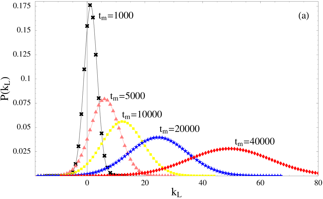
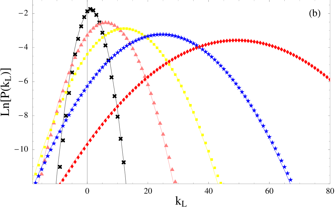
In Fig. 2a, we display the probability distribution of the net number of electron kLsubscript𝑘𝐿k_{L} which have crossed the left lead-system interface for different measurement times and for a fixed temperature and bias. The logarithmic plot in Fig. 2b highlights the tails of the distribution. Positive (negative) kLsubscript𝑘𝐿k_{L} represent electrons which move in the direction favored (unfavored) by the bias. As the measurement time increases, the average of the probability distribution moves to the positive direction linearly in time at a speed given by the steady state current. As expected, the longer the measurement time, the smaller the probability of observing a current flowing against the bias. Since the FT applies in the long times limit, this shows that the FT quantifies the rare fluctuations described by the tails of the probability distribution.

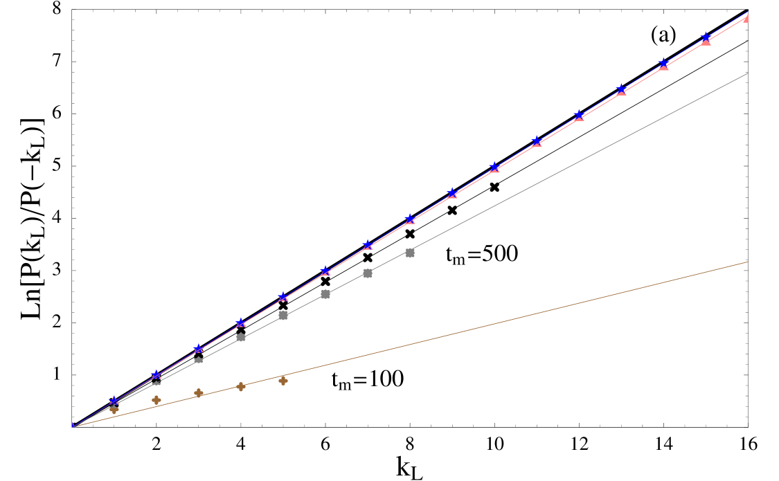
Fig. 3a, shows the logarithm of P(t,kL)/P(t,kL)𝑃𝑡subscript𝑘𝐿𝑃𝑡subscript𝑘𝐿P(t,k_{L})/P(t,-k_{L}) for different measurement times. The longer the time, the closer the results from the FT. The numerical results suggest that for finite times

P(t,k)P(t,k)e(βeVαt)k,𝑃𝑡𝑘𝑃𝑡𝑘superscript𝑒𝛽𝑒𝑉subscript𝛼𝑡𝑘\displaystyle\frac{P(t,k)}{P(t,-k)}\approx e^{(\beta eV-\alpha_{t})k}\;, (40)

where limtαt=0subscript𝑡subscript𝛼𝑡0\lim_{t\to\infty}\alpha_{t}=0. This form is not valid for very short measurement time, but seems to be a very good approximation for times after which the probability to measure at least a few electron transfers become significant.

To calculate αtsubscript𝛼𝑡\alpha_{t}, we note that using (24), Eq. (40) implies that

G(t,λL)G(t,βeVαtλL).𝐺𝑡subscript𝜆𝐿𝐺𝑡𝛽𝑒𝑉subscript𝛼𝑡subscript𝜆𝐿\displaystyle G(t,\lambda_{L})\approx G(t,\beta eV-\alpha_{t}-\lambda_{L})\;. (41)

Since we do not consider very short times, (28) can be very well approximated by

lnG(t,λL)gm0(λL)t+B(λL),𝐺𝑡subscript𝜆𝐿subscript𝑔subscript𝑚0subscript𝜆𝐿𝑡𝐵subscript𝜆𝐿\displaystyle\ln G(t,\lambda_{L})\approx g_{m_{0}}(\lambda_{L})t+B(\lambda_{L})\;, (42)

where m0subscript𝑚0m_{0} is the index of the eigenvalue with the smallest absolute value and

B(λL)𝐵subscript𝜆𝐿\displaystyle B(\lambda_{L}) \displaystyle\equiv ln(I|gm0(λL)g~m0(λL)|ρ(0)).\displaystyle\ln\big{(}\ll I|g_{m_{0}}(\lambda_{L})\gg\ll\tilde{g}_{m_{0}}(\lambda_{L})|\rho(0)\gg\big{)}\;. (43)

Since G(t,0)=G(t,βeVαt)=1𝐺𝑡0𝐺𝑡𝛽𝑒𝑉subscript𝛼𝑡1G(t,0)=G(t,\beta eV-\alpha_{t})=1, we find that

gm0(βeVαt)tB(βeVαt).subscript𝑔subscript𝑚0𝛽𝑒𝑉subscript𝛼𝑡𝑡𝐵𝛽𝑒𝑉subscript𝛼𝑡\displaystyle g_{m_{0}}(\beta eV-\alpha_{t})t\approx-B(\beta eV-\alpha_{t})\;. (44)

If we consider long enough times for which αtβeVmuch-less-thansubscript𝛼𝑡𝛽𝑒𝑉\alpha_{t}\ll\beta eV and αt/t0subscript𝛼𝑡𝑡0\alpha_{t}/t\approx 0, using a first [zero] order expansion of gm0(βeVαt)subscript𝑔subscript𝑚0𝛽𝑒𝑉subscript𝛼𝑡g_{m_{0}}(\beta eV-\alpha_{t}) [B(βeVαt)𝐵𝛽𝑒𝑉subscript𝛼𝑡B(\beta eV-\alpha_{t})] around βeV𝛽𝑒𝑉\beta eV and using (95), we get

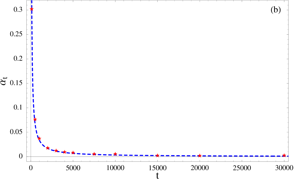
αtB(βeV)eIηst1t.subscript𝛼𝑡𝐵𝛽𝑒𝑉𝑒subscriptdelimited-⟨⟩subscript𝐼𝜂st1𝑡\displaystyle\alpha_{t}\approx\frac{B(\beta eV)}{e\langle I_{\eta}\rangle_{\rm st}}\frac{1}{t}\;. (45)

The average current can be calculated using Ist=sMIsstsubscriptdelimited-⟨⟩𝐼stsuperscriptsubscript𝑠𝑀subscriptdelimited-⟨⟩subscript𝐼𝑠st\langle I\rangle_{\rm st}=\sum_{s}^{M}\langle I_{s}\rangle_{\rm st} and (34). Using B(λL)=sMB(λ(L,s))𝐵subscript𝜆𝐿superscriptsubscript𝑠𝑀𝐵subscript𝜆𝐿𝑠B(\lambda_{L})=\sum_{s}^{M}B(\lambda_{(L,s)}), where B(λ(L,s))=ln(I|g(λ(L,s))g~(λL,s)|ρ(0))B(\lambda_{(L,s)})=\ln\big{(}\ll I|g_{-}(\lambda_{(L,s)})\gg\ll\tilde{g}_{-}(\lambda_{L,s})|\rho(0)\gg\big{)} and ρ(0)𝜌0\rho(0) correspond to steady state, we find that

B(βeV)=sMln(vss(L)+eβeVwss(L))(eβeVwss(L)(wss(L)+wss(R))2+vss(L)(wss(L)+eβeVwss(R))2)(eβeVvss(L)wss(R)+wss(L)(vss(L)+wss(L)+wss(R)))2.𝐵𝛽𝑒𝑉superscriptsubscript𝑠𝑀superscriptsubscript𝑣𝑠𝑠𝐿superscript𝑒𝛽𝑒𝑉superscriptsubscript𝑤𝑠𝑠𝐿superscript𝑒𝛽𝑒𝑉superscriptsubscript𝑤𝑠𝑠𝐿superscriptsuperscriptsubscript𝑤𝑠𝑠𝐿superscriptsubscript𝑤𝑠𝑠𝑅2superscriptsubscript𝑣𝑠𝑠𝐿superscriptsuperscriptsubscript𝑤𝑠𝑠𝐿superscript𝑒𝛽𝑒𝑉superscriptsubscript𝑤𝑠𝑠𝑅2superscriptsuperscript𝑒𝛽𝑒𝑉superscriptsubscript𝑣𝑠𝑠𝐿superscriptsubscript𝑤𝑠𝑠𝑅superscriptsubscript𝑤𝑠𝑠𝐿superscriptsubscript𝑣𝑠𝑠𝐿superscriptsubscript𝑤𝑠𝑠𝐿superscriptsubscript𝑤𝑠𝑠𝑅2\displaystyle B(\beta eV)=\sum_{s}^{M}\ln\frac{(v_{ss}^{(L)}+e^{-\beta eV}w_{ss}^{(L)})\big{(}e^{\beta eV}w_{ss}^{(L)}(w_{ss}^{(L)}+w_{ss}^{(R)})^{2}+v_{ss}^{(L)}(w_{ss}^{(L)}+e^{\beta eV}w_{ss}^{(R)})^{2}\big{)}}{\big{(}e^{\beta eV}v_{ss}^{(L)}w_{ss}^{(R)}+w_{ss}^{(L)}(v_{ss}^{(L)}+w_{ss}^{(L)}+w_{ss}^{(R)})\big{)}^{2}}\;. (46)

Notice that since exp{B(λ(L,s))}1𝐵subscript𝜆𝐿𝑠1\exp{\{B(\lambda_{(L,s)})\}}\geq 1, then αt0subscript𝛼𝑡0\alpha_{t}\geq 0 (the equality only holds when βeV=0𝛽𝑒𝑉0\beta eV=0).

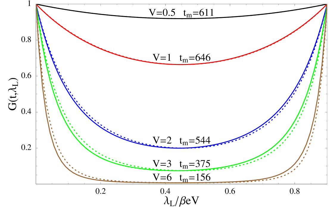
Figure 3b shows that our estimate for αtsubscript𝛼𝑡\alpha_{t} is in excellent agreement with the values obtained by linearly fitting the results of Fig. 3a. It should be noted that the results presented on Fig. 2-3 correspond to small bias. For larger bias the probability of the backward processes P(k)𝑃𝑘P(-k) becomes very small which limits the numerical accuracy. However, the GF is still numerically accessible for high bias. Fig. 4 shows that the GF symmetry (41) on which our methods relies is not perfectly preserved for larger bias. It is therefore expected that the accuracy of our method decreases with increasing bias.

One can see on Fig. 2 that the probability distribution can be reasonably well fitted by a Gaussian. Deviations can be observed at very short times or for the tails of the distributions. The GF of a Gaussian probability distribution P(t,k)=(2πσt2)1/2exp{(kkt)2/(2σt2)}𝑃𝑡𝑘superscript2𝜋subscriptsuperscript𝜎2𝑡12superscript𝑘subscriptdelimited-⟨⟩𝑘𝑡22subscriptsuperscript𝜎2𝑡P(t,k)=(2\pi\sigma^{2}_{t})^{-1/2}\exp{\{-(k-\langle k\rangle_{t})^{2}/(2\sigma^{2}_{t})\}} is given by G(t,λ)=exp{λ2σt2/2λkt}𝐺𝑡𝜆superscript𝜆2subscriptsuperscript𝜎2𝑡2𝜆subscriptdelimited-⟨⟩𝑘𝑡G(t,\lambda)=\exp{\{\lambda^{2}\sigma^{2}_{t}/2-\lambda\langle k\rangle_{t}\}}. The nonzero solution of G(t,λ)=1𝐺𝑡𝜆1G(t,\lambda)=1 is λ0=2kt/σt2=2/F(t)subscript𝜆02subscriptdelimited-⟨⟩𝑘𝑡subscriptsuperscript𝜎2𝑡2𝐹𝑡\lambda_{0}=2\langle k\rangle_{t}/\sigma^{2}_{t}=2/F(t), where F(t)𝐹𝑡F(t) is the time dependent Fano parameter associated with the net number of charge transferred through an interface. The GF has the symmetry G(t,λ)=G(t,λ0λ)𝐺𝑡𝜆𝐺𝑡subscript𝜆0𝜆G(t,\lambda)=G(t,\lambda_{0}-\lambda). Using the results of section V to calculate F()𝐹F(\infty), we find that for very long measurement times λ0=βeV+𝒪(V3)subscript𝜆0𝛽𝑒𝑉𝒪superscript𝑉3\lambda_{0}=\beta eV+{\cal O}(V^{3}). This indicates that it is only in the low bias limit that the Gaussian approximation can be trusted for describing the tails of the probability distribution which characterize the FT. This was confirmed by numerically studying the GF. We finally notice that our estimate of αtsubscript𝛼𝑡\alpha_{t} is exact when the Gaussian approximation is satisfied, but can also be applied to non-Gaussian distributions as long as (40) or (41) remains a good assumption.

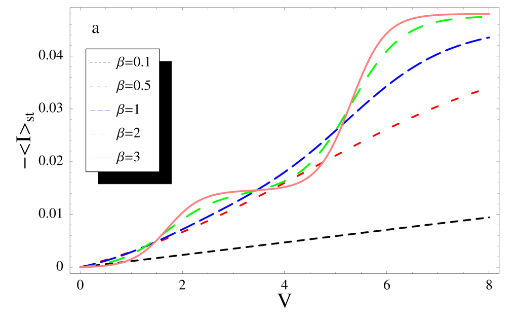
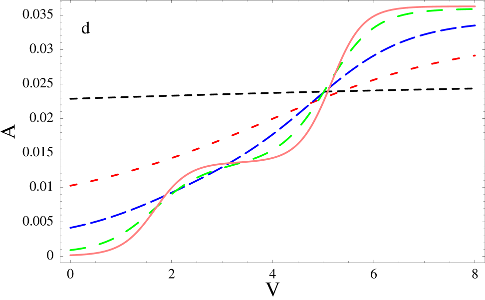
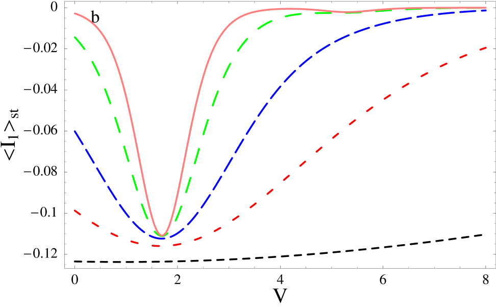
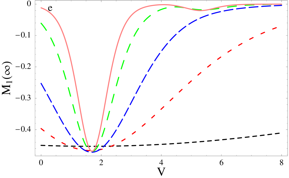
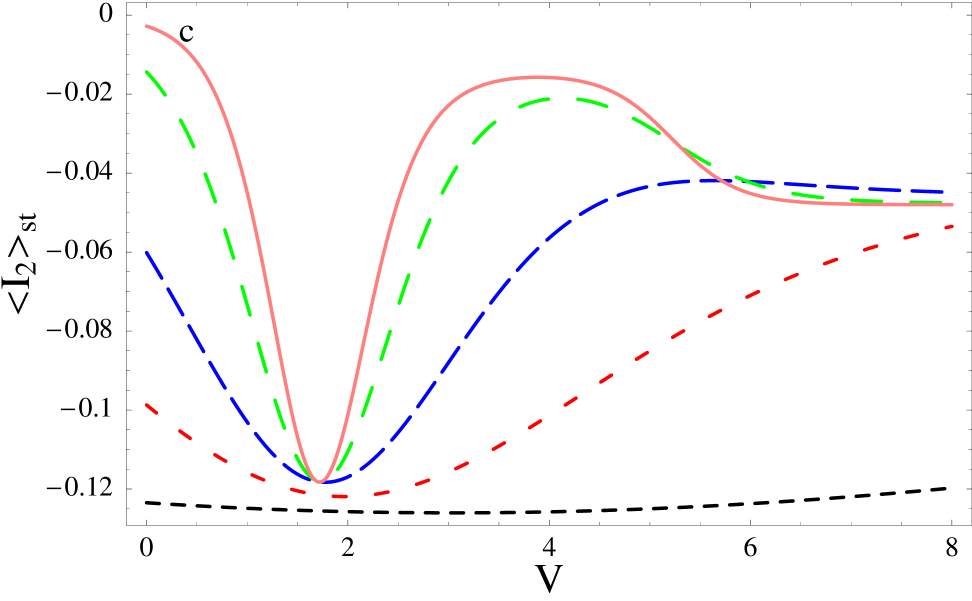
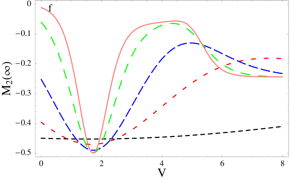
The average steady-state current associated with the net number of electrons crossing a given junction interface is plotted as a function of the bias in Fig. 5a. This typical current-voltage characteristic shows that the current increases by steps each time the bias is large enough to make a new orbital contribute to the current (when eV=ϵ1=1.697𝑒𝑉subscriptitalic-ϵ11.697eV=\epsilon_{1}=1.697 or eV=ϵ2=5.303𝑒𝑉subscriptitalic-ϵ25.303eV=\epsilon_{2}=5.303). The current associated with the process η=1𝜂1\eta=1 and η=2𝜂2\eta=2 is plotted on Fig. 5b and 5c. The current on Fig. 5a is given by the difference between Fig. 5c and Fig. 5b. Temperature, when increased, has the effect of smoothing these steps and reducing the current because thermal fluctuations tend to equalize the forward and backward currents. Ohm’s law is recovered for β(ϵ2ϵ1)<1𝛽subscriptitalic-ϵ2subscriptitalic-ϵ11\beta(\epsilon_{2}-\epsilon_{1})<1. The zero frequency power spectrum associated to the total net current through a system interface is plotted as a function of the bias in Fig. 5d. The Mandel parameter associated with the η=1𝜂1\eta=1 and η=2𝜂2\eta=2 processes is plotted in Fig. 5e and 5f. We see that the deviations from Poisson statistics are always strong and tend to vanish only when the currents associated with η=1𝜂1\eta=1 and η=2𝜂2\eta=2 vanish. This indicates that the various type of electron transfer are highly correlated with each other. The Mandel parameter is always negative, indicating subpoissonian (antibunching) statistics. This has been experimentally observed in Hirayama .

VII Discussion

Many different types of fluctuation theorems (FT) have been derived for stochastic dynamical systems. These differ by the mechanism used to drive the system out of equilibrium. In the first case Crooks99 ; Crooks00 ; Seifert , the system is closed and driven by a time-dependent force which makes the rate matrix of the birth and death master equation time dependent. When the driving stops, the system will eventually reach equilibrium because the rate matrix is detailed balanced Crooks99 . In the second case Lebowitz ; Gaspard1 ; Seifert ; Maes2 , the system is open and the the rate matrix is not detailed balanced. Even without driving, the system will eventually reach a nonequilibrium steady state. A third class of FT Hatano99 ; Hatano01 ; Bustamante04 considers the fluctuation of an entropy associated with the excess heat produced when a time dependent driving induces transitions between different nonequilibrium steady states. This paper focuses on the second case.

So far, we have assumed that the two leads of the junction have the same temperature but different chemical potentials μL=μ0+Δμsubscript𝜇𝐿subscript𝜇0Δ𝜇\mu_{L}=\mu_{0}+\Delta\mu and μR=μ0subscript𝜇𝑅subscript𝜇0\mu_{R}=\mu_{0}. One could wonder what happens to the FT if one considers different temperatures for the two leads βL=β0+Δβ=subscript𝛽𝐿subscript𝛽0Δ𝛽absent\beta_{L}=\beta_{0}+\Delta\beta= and βR=β0subscript𝛽𝑅subscript𝛽0\beta_{R}=\beta_{0}. In such case, the argument of the exponential on the r.h.s. of (5) becomes xβ0ΔμΔβ(ϵsμ0)+ΔβΔμ𝑥subscript𝛽0Δ𝜇Δ𝛽subscriptitalic-ϵ𝑠subscript𝜇0Δ𝛽Δ𝜇x\equiv\beta_{0}\Delta\mu-\Delta\beta(\epsilon_{s}-\mu_{0})+\Delta\beta\Delta\mu. This implies for the orbital GF that the analogue of the symmetry (27) becomes Ss(λ(y,s))=Ss(xλ(y,s))subscript𝑆𝑠subscript𝜆𝑦𝑠subscript𝑆𝑠𝑥subscript𝜆𝑦𝑠S_{s}(\lambda_{(y,s)})=S_{s}(x-\lambda_{(y,s)}). However, since x𝑥x is different for each orbital (due to ϵssubscriptitalic-ϵ𝑠\epsilon_{s}), the many body GF, which is given by the sum of the orbital GFs, does not possess the analogue of the symmetry (29). It is therefore only for a single orbital model that a FT P(t,k)/P(t,k)=exp{xk}𝑃𝑡𝑘𝑃𝑡𝑘𝑥𝑘P(t,k)/P(t,-k)=\exp{\{xk\}} holds.

In summary, we have applied the quantum master equation derived in HarbolaEsposito for calculating the counting statistics of electrons tunneling through a quantum junction made of a system embedded between two leads. Using a generating function formalism, we derived an evolution equation for the generating operator which allows to calculate the time dependent probability distribution of electron transfer events. This equation can be solved analytically because the many-body generating operator is a product of single orbital generating operators. We then demonstrated that the net number of electrons crossing a given system-lead interface satisfies a FT at long times. This implies that measuring a net number of electron transfer in the direction favored by the bias is exponentially more probable than measuring it in the opposite direction. Since the argument in the exponential is the work needed to transfer the measured electrons through the junction, this fluctuation theorem can be viewed as a Crooks relation Crooks99 ; Crooks00 . We furthermore described how the moments of the current distribution can be deduced from the electron counting statistics and gave analytical expressions for currents and power spectra. Numerically calculations of the probability distribution for the electron counts for a model of two coupled quantum dots demonstrated that the FT becomes valid for long measurement times. A method to calculate the finite-time deviations was proposed.

Several future extensions of this work are called for. The first one is to find if electron-electron interactions affect the FT. Another one is to investigate if the FT still holds in a system where the population dynamics couple to the coherence dynamics (e.g. a quantum junction externally driven by a laser). In analogy to the excess heat Hatano01 , one could also consider fluctuations of excess currents, produced during transition between steady-states.

Acknowledgment

The support of the National Science Foundation (Grant No. CHE-0446555) and NIRT (Grant No. EEC 0303389) is gratefully acknowledged. M. E. is partially supported by the FNRS Belgium (collaborateur scientifique).

Appendix A Trajectory picture for the QME dynamics

Using the interaction representation, we can recast Eq. (6) as

|ρ˙I(t)=Γ^(t)|ρI(t),\displaystyle|\dot{\rho}_{I}(t)\gg=\hat{\Gamma}(t)|\rho_{I}(t)\gg\;, (47)

where

|ρI(t)𝒰^0(0,t)|ρ(t)\displaystyle|\rho_{I}(t)\gg\equiv\hat{{\cal U}}_{0}(0,t)|\rho(t)\gg (48)

and

Γ^(t)=𝒰^0(0,t)Γ^𝒰^0(t,0),^Γ𝑡subscript^𝒰00𝑡^Γsubscript^𝒰0𝑡0\displaystyle\hat{\Gamma}(t)=\hat{{\cal U}}_{0}(0,t)\hat{\Gamma}\hat{{\cal U}}_{0}(t,0)\;, (49)

where 𝒰^0(0,t)exp[^0t]subscript^𝒰00𝑡subscript^0𝑡\hat{{\cal U}}_{0}(0,t)\equiv\exp{[-\hat{{\cal M}}_{0}t]}. ^0=^+γ^subscript^0^^𝛾\hat{{\cal M}}_{0}=\hat{{\cal L}}+\hat{\gamma} describes the system dynamics in absence of electron transfer. The formal solution of (47) reads

|ρI(t)\displaystyle|\rho_{I}(t)\gg =\displaystyle= exp+[0tdτΓ^(τ)]|ρI(0)=k=0|ρI(k)(t),\displaystyle\exp_{+}{[\int_{0}^{t}d\tau\hat{{\Gamma}}(\tau)]}|\rho_{I}(0)\gg=\sum_{k=0}^{\infty}|\rho^{(k)}_{I}(t)\gg\;, (50)

where

|ρI(k)(t)=0tdτk0τkdτk10τ2dτ1Γ^(τk)Γ^(τk1)Γ^(τ1)|ρI(0)=0tdτΓ^(τ)|ρI(k1)(τ).\displaystyle|\rho^{(k)}_{I}(t)\gg=\int_{0}^{t}d\tau_{k}\int_{0}^{\tau_{k}}d\tau_{k-1}\ldots\int_{0}^{\tau_{2}}d\tau_{1}\hat{\Gamma}(\tau_{k})\hat{\Gamma}(\tau_{k-1})\ldots\hat{\Gamma}(\tau_{1})|\rho_{I}(0)\gg=\int_{0}^{t}d\tau\hat{\Gamma}(\tau)|\rho^{(k-1)}_{I}(\tau)\gg\;. (51)

Multiplying Eq. (51) by 𝒰^0(t,0)subscript^𝒰0𝑡0\hat{{\cal U}}_{0}(t,0), we get

|ρ(k)(t)=0tdτk0τkdτk10τ2dτ1𝒰^0(t,τk)Γ^𝒰^0(τk,τk1)Γ^𝒰^0(τ2,τ1)Γ^𝒰^0(τ1,0)|ρ(0).\displaystyle|\rho^{(k)}(t)\gg=\int_{0}^{t}d\tau_{k}\int_{0}^{\tau_{k}}d\tau_{k-1}\ldots\int_{0}^{\tau_{2}}d\tau_{1}\hat{{\cal U}}_{0}(t,\tau_{k})\hat{\Gamma}\hat{{\cal U}}_{0}(\tau_{k},\tau_{k-1})\hat{\Gamma}\ldots\hat{{\cal U}}_{0}(\tau_{2},\tau_{1})\hat{\Gamma}\hat{{\cal U}}_{0}(\tau_{1},0)|\rho(0)\gg\;. (52)

This is the density matrix conditional to the transfer of k𝑘k electrons between the system and the leads, irrespective of the type of transfer η𝜂\eta or orbital s𝑠s.

We shall denote the number of electron transfers of type η𝜂\eta through the s𝑠s orbital by kνsubscript𝑘𝜈k_{\nu} where ν=(η,s)𝜈𝜂𝑠\nu=(\eta,s). The number of electron transfers of type η𝜂\eta disregarding the orbital is kη=s=1Mk(η,s)subscript𝑘𝜂superscriptsubscript𝑠1𝑀subscript𝑘𝜂𝑠k_{\eta}=\sum_{s=1}^{M}k_{(\eta,s)} and the number of electron transfer through the orbital s𝑠s disregarding the type of transfer is ks=η=14k(η,s)subscript𝑘𝑠superscriptsubscript𝜂14subscript𝑘𝜂𝑠k_{s}=\sum_{\eta=1}^{4}k_{(\eta,s)}. We have that k=νkν𝑘subscript𝜈subscript𝑘𝜈k=\sum_{\nu}k_{\nu}. We define

𝕜=k(1,1),k(1,2),,k(1,M),k(2,1),k(2,2),,k(2,M),,k(4,1),k(4,2),,k(4,M)𝕜subscript𝑘11subscript𝑘12subscript𝑘1𝑀subscript𝑘21subscript𝑘22subscript𝑘2𝑀subscript𝑘41subscript𝑘42subscript𝑘4𝑀\displaystyle\mathbb{k}=k_{(1,1)},k_{(1,2)},\cdots,k_{(1,M)},k_{(2,1)},k_{(2,2)},\cdots,k_{(2,M)},\cdots,k_{(4,1)},k_{(4,2)},\cdots,k_{(4,M)} (53)
𝕜s=k(1,s),k(2,s),k(3,s),k(4,s)subscript𝕜𝑠subscript𝑘1𝑠subscript𝑘2𝑠subscript𝑘3𝑠subscript𝑘4𝑠\displaystyle\mathbb{k}_{s}=k_{(1,s)},k_{(2,s)},k_{(3,s)},k_{(4,s)}
𝕜η=k(η,1),k(η,2),,k(η,M).subscript𝕜𝜂subscript𝑘𝜂1subscript𝑘𝜂2subscript𝑘𝜂𝑀\displaystyle\mathbb{k}_{\eta}=k_{(\eta,1)},k_{(\eta,2)},\cdots,k_{(\eta,M)}\;.

A trajectory (ν,t)(τ)subscript𝜈𝑡𝜏(\nu,t)_{(\tau)} records (from left to right) the sequence of electron transfer events during a time τ𝜏\tau, by labeling them according to the type of transfer, the relevant orbital and the time at which a given transfer occurs (ν,t)(τ)=(ν1,t1),(ν2,t2),,(νk,tk)subscript𝜈𝑡𝜏subscript𝜈1subscript𝑡1subscript𝜈2subscript𝑡2subscript𝜈𝑘subscript𝑡𝑘(\nu,t)_{(\tau)}=(\nu_{1},t_{1}),(\nu_{2},t_{2}),\cdots,(\nu_{k},t_{k}). A sequence (ν)(τ)subscript𝜈𝜏(\nu)_{(\tau)} is a trajectory where the transfer time is not recorded (ν)(τ)=ν1,ν2,,νksubscript𝜈𝜏subscript𝜈1subscript𝜈2subscript𝜈𝑘(\nu)_{(\tau)}=\nu_{1},\nu_{2},\cdots,\nu_{k}.
We can now decompose ρI(t)subscript𝜌𝐼𝑡\rho_{I}(t) as

|ρI(t)=𝕜|ρI(𝕜)(t),\displaystyle|\rho_{I}(t)\gg=\sum_{\mathbb{k}}|\rho_{I}^{(\mathbb{k})}(t)\gg\;, (54)

where the sum is over all the component kνsubscript𝑘𝜈k_{\nu} of 𝕜𝕜\mathbb{k} and runs from zero to infnity. Using (12), the probability to measure 𝕜𝕜\mathbb{k} electrons transferred to the leads at time t𝑡t is given by

P(t,𝕜)𝑃𝑡𝕜\displaystyle P(t,\mathbb{k}) =\displaystyle= I|𝒰^0(t,0)|ρI(𝕜)(t).much-less-thanabsent𝐼subscript^𝒰0𝑡0superscriptsubscript𝜌𝐼𝕜𝑡much-greater-thanabsent\displaystyle\ll I|\hat{{\cal U}}_{0}(t,0)|\rho_{I}^{(\mathbb{k})}(t)\gg\;. (55)

The master equation (6) preserves the trace so that the normalization condition 𝕜P(t,𝕜)=1subscript𝕜𝑃𝑡𝕜1\sum_{\mathbb{k}}P(t,\mathbb{k})=1 is satisfied.

We next define the elementary probability density of a given trajectory (ν,τ)(t)subscript𝜈𝜏𝑡(\nu,\tau)_{(t)} which contains k𝑘k electron transfer events at time τ1,,τksubscript𝜏1subscript𝜏𝑘\tau_{1},\ldots,\tau_{k} during a time interval t𝑡t as

Π[(ν,τ)(t)]Tr|𝒰^0(t,0)Γ^νk(τk)Γ^νk1(τk1)Γ^ν1(τ1)|ρI(0).\displaystyle\Pi[(\nu,\tau)_{(t)}]\equiv\ll{\rm Tr}|\hat{{\cal U}}_{0}(t,0)\hat{\Gamma}_{\nu_{k}}(\tau_{k})\hat{\Gamma}_{\nu_{k-1}}(\tau_{k-1})\ldots\hat{\Gamma}_{\nu_{1}}(\tau_{1})|\rho_{I}(0)\gg\;. (56)

The probability of a sequence (ν)(t)subscript𝜈𝑡(\nu)_{(t)} with k𝑘k events is obtained by time integrating (56)

Π[(ν)(t)]Πdelimited-[]subscript𝜈𝑡\displaystyle\Pi[(\nu)_{(t)}] =\displaystyle= 0t𝑑τk0τk𝑑τk10τ2𝑑τ1Π[(ν,τ)(t)].superscriptsubscript0𝑡differential-dsubscript𝜏𝑘superscriptsubscript0subscript𝜏𝑘differential-dsubscript𝜏𝑘1superscriptsubscript0subscript𝜏2differential-dsubscript𝜏1Πdelimited-[]subscript𝜈𝜏𝑡\displaystyle\int_{0}^{t}d\tau_{k}\int_{0}^{\tau_{k}}d\tau_{k-1}\ldots\int_{0}^{\tau_{2}}d\tau_{1}\Pi[(\nu,\tau)_{(t)}]\;. (57)

Using Eq. (52), and since our equation conserves the trace, we see that (ν)(t)Π[(ν)(t)]=1subscriptsubscript𝜈𝑡Πdelimited-[]subscript𝜈𝑡1\sum_{(\nu)_{(t)}}\Pi[(\nu)_{(t)}]=1, where (ν)(t)subscriptsubscript𝜈𝑡\sum_{(\nu)_{(t)}} is the sum over all possible electron transfer sequences (without keeping track of transfer times). The trace of (51) can now be written using (56) and (57) as

P(t,𝕜)=(ν)(t)𝕜Π[(ν)(t)],𝑃𝑡𝕜subscriptsubscript𝜈𝑡𝕜Πdelimited-[]subscript𝜈𝑡\displaystyle P(t,\mathbb{k})=\sum_{(\nu)_{(t)}\in\mathbb{k}}\Pi[(\nu)_{(t)}]\;, (58)

where the summation is restricted to sequences such that the number of transfer events is 𝕜𝕜\mathbb{k}.
Because a number 𝕜𝕜\mathbb{k} of electrons at time t𝑡t can be realized by the four types of electron transfer processes (Fig. 1) and via M𝑀M different orbitals, we have

|ρI(𝕜)(t)\displaystyle|\rho_{I}^{(\mathbb{k})}(t)\gg =\displaystyle= ν0t𝑑τΓ^ν(τ)|ρI(𝕜𝟙ν)(τ),much-greater-thanconditionalsubscript𝜈superscriptsubscript0𝑡differential-d𝜏subscript^Γ𝜈𝜏superscriptsubscript𝜌𝐼𝕜subscript1𝜈𝜏absent\displaystyle\sum_{\nu}\int_{0}^{t}d\tau\hat{\Gamma}_{\nu}(\tau)|\rho_{I}^{(\mathbb{k}-\mathbb{1}_{\nu})}(\tau)\gg\;, (59)

where 𝟙ν=0,,0,1,0,,0subscript1𝜈00100\mathbb{1}_{\nu}=0,\cdots,0,1,0,\cdots,0, where 111 is at the position ν𝜈\nu in the sequence.
Using the interaction picture of the GO, we can rewrite (59) as

|GI(t,𝝀)=0tdτ(νeλνΓ^ν(τ))|GI(τ,𝝀).\displaystyle|G_{I}(t,\bm{\lambda})\gg=\int_{0}^{t}d\tau\big{(}\sum_{\nu}e^{\lambda_{\nu}}\hat{\Gamma}_{\nu}(\tau)\big{)}|G_{I}(\tau,\bm{\lambda})\gg\;. (60)

By taking the time derivative and going back to the Schrödinger picture, we get Eq. (16).

Appendix B Solution of the GF

The generator of (16) can be written as a sum of contributions of each orbital

𝒲^(𝝀)=s=1M𝒲^s(𝝀s),^𝒲𝝀superscriptsubscript𝑠1𝑀subscript^𝒲𝑠subscript𝝀𝑠\displaystyle\hat{{\cal W}}(\bm{\lambda})=\sum_{s=1}^{M}\hat{{\cal W}}_{s}(\bm{\lambda}_{s})\;, (61)

where

𝒲^s(𝝀s)=^s+γ^s+η=14eλ(η,s)Γ^(η,s)subscript^𝒲𝑠subscript𝝀𝑠subscript^𝑠subscript^𝛾𝑠superscriptsubscript𝜂14superscript𝑒subscript𝜆𝜂𝑠subscript^Γ𝜂𝑠\displaystyle\hat{{\cal W}}_{s}(\bm{\lambda}_{s})=\hat{{\cal L}}_{s}+\hat{\gamma}_{s}+\sum_{\eta=1}^{4}e^{\lambda_{(\eta,s)}}\hat{\Gamma}_{(\eta,s)} (62)

and ^siϵs[cscs,]subscript^𝑠𝑖subscriptitalic-ϵ𝑠superscriptsubscript𝑐𝑠subscript𝑐𝑠\hat{{\cal L}}_{s}\equiv-i\epsilon_{s}[c_{s}^{\dagger}c_{s},\cdot]. The GO can therefore be factorized as a tensor product of orbital GO

|G(t,𝝀)=s=1M|Gs(t,𝝀s),\displaystyle|G(t,\bm{\lambda})\gg=\prod_{s=1}^{M}|G_{s}(t,\bm{\lambda}_{s})\gg\otimes\;, (63)

which evolve independently according to

|G˙s(t,𝝀s)=𝒲^s(𝝀s)|Gs(t,𝝀s).\displaystyle|\dot{G}_{s}(t,\bm{\lambda}_{s})\gg=\hat{{\cal W}}_{s}(\bm{\lambda}_{s})|G_{s}(t,\bm{\lambda}_{s})\gg\;. (64)

Projecting Eq. (64) into the system eigenbasis and using the notation

n1nM;n1nM|G(t,𝝀)=s=1Mns;ns|Gs(t,𝝀s)=s=1MGns;ns(t,𝝀s),\displaystyle\ll n_{1}\cdots n_{M};n_{1}^{\prime}\cdots n_{M}^{\prime}|G(t,\bm{\lambda})\gg=\prod_{s=1}^{M}\ll n_{s};n_{s}^{\prime}|G_{s}(t,\bm{\lambda}_{s})\gg=\prod_{s=1}^{M}G_{n_{s};n_{s}^{\prime}}(t,\bm{\lambda}_{s})\;, (65)

we get

(G˙1;1(t,𝝀s)G˙0;0(t,𝝀s)G˙1;0(t,𝝀s)G˙0;1(t,𝝀s))=𝒲^(𝝀s)(G1;1(t,𝝀s)G0;0(t,𝝀s)G1;0(t,𝝀s)G0;1(t,𝝀s)),subscript˙𝐺11𝑡subscript𝝀𝑠subscript˙𝐺00𝑡subscript𝝀𝑠subscript˙𝐺10𝑡subscript𝝀𝑠subscript˙𝐺01𝑡subscript𝝀𝑠^𝒲subscript𝝀𝑠subscript𝐺11𝑡subscript𝝀𝑠subscript𝐺00𝑡subscript𝝀𝑠subscript𝐺10𝑡subscript𝝀𝑠subscript𝐺01𝑡subscript𝝀𝑠\displaystyle\left(\begin{array}[]{c}\dot{G}_{1;1}(t,\bm{\lambda}_{s})\\ \dot{G}_{0;0}(t,\bm{\lambda}_{s})\\ \dot{G}_{1;0}(t,\bm{\lambda}_{s})\\ \dot{G}_{0;1}(t,\bm{\lambda}_{s})\\ \end{array}\right)=\hat{{\cal W}}(\bm{\lambda}_{s})\left(\begin{array}[]{c}G_{1;1}(t,\bm{\lambda}_{s})\\ G_{0;0}(t,\bm{\lambda}_{s})\\ G_{1;0}(t,\bm{\lambda}_{s})\\ G_{0;1}(t,\bm{\lambda}_{s})\\ \end{array}\right)\;, (74)

where

𝒲^(𝝀s)=2(vsseλ(2,s)wss(L)+eλ(4,s)wss(R)00eλ(1,s)vss(L)+eλ(3,s)vss(R)wss0000iϵsvsswss0000iϵsvsswss).^𝒲subscript𝝀𝑠2subscript𝑣𝑠𝑠superscript𝑒subscript𝜆2𝑠superscriptsubscript𝑤𝑠𝑠𝐿superscript𝑒subscript𝜆4𝑠superscriptsubscript𝑤𝑠𝑠𝑅00superscript𝑒subscript𝜆1𝑠superscriptsubscript𝑣𝑠𝑠𝐿superscript𝑒subscript𝜆3𝑠superscriptsubscript𝑣𝑠𝑠𝑅subscript𝑤𝑠𝑠0000𝑖subscriptitalic-ϵ𝑠subscript𝑣𝑠𝑠subscript𝑤𝑠𝑠0000𝑖subscriptitalic-ϵ𝑠subscript𝑣𝑠𝑠subscript𝑤𝑠𝑠\displaystyle\hat{{\cal W}}(\bm{\lambda}_{s})=2\left(\begin{array}[]{cccc}-v_{ss}&e^{\lambda_{(2,s)}}w_{ss}^{(L)}+e^{\lambda_{(4,s)}}w_{ss}^{(R)}&0&0\\ e^{\lambda_{(1,s)}}v_{ss}^{(L)}+e^{\lambda_{(3,s)}}v_{ss}^{(R)}&-w_{ss}&0&0\\ 0&0&-i\epsilon_{s}-v_{ss}-w_{ss}&0\\ 0&0&0&i\epsilon_{s}-v_{ss}-w_{ss}\end{array}\right)\;. (79)

Since we work in the reduced Liouville space (where FSC are neglected), only the coherences such that s=1Mns=s=1Mnssuperscriptsubscript𝑠1𝑀subscript𝑛𝑠superscriptsubscript𝑠1𝑀superscriptsubscript𝑛𝑠\sum_{s=1}^{M}n_{s}=\sum_{s=1}^{M}n_{s}^{\prime} are kept in (65).

The two eigenvalues of the generator (79) corresponding to the population dynamics are given by

g±(𝝀s)subscript𝑔plus-or-minussubscript𝝀𝑠\displaystyle g_{\pm}(\bm{\lambda}_{s}) =\displaystyle= (vss+wss2)±(vss+wss2)2+f(𝝀s),plus-or-minussubscript𝑣𝑠𝑠subscript𝑤𝑠𝑠2superscriptsubscript𝑣𝑠𝑠subscript𝑤𝑠𝑠22𝑓subscript𝝀𝑠\displaystyle-\left(\frac{v_{ss}+w_{ss}}{2}\right)\pm\sqrt{\left(\frac{v_{ss}+w_{ss}}{2}\right)^{2}+f(\bm{\lambda}_{s})}\;, (80)

where

f(𝝀s)𝑓subscript𝝀𝑠\displaystyle f(\bm{\lambda}_{s}) =\displaystyle= vss(L){(e(λ(1,s)+λ(2,s))1)wss(L)+(e(λ(1,s)+λ(4,s))1)wss(R)}superscriptsubscript𝑣𝑠𝑠𝐿superscript𝑒subscript𝜆1𝑠subscript𝜆2𝑠1superscriptsubscript𝑤𝑠𝑠𝐿superscript𝑒subscript𝜆1𝑠subscript𝜆4𝑠1superscriptsubscript𝑤𝑠𝑠𝑅\displaystyle v_{ss}^{(L)}\{(e^{(\lambda_{(1,s)}+\lambda_{(2,s)})}-1)w_{ss}^{(L)}+(e^{(\lambda_{(1,s)}+\lambda_{(4,s)})}-1)w_{ss}^{(R)}\}
+vss(R){(e(λ(2,s)+λ(3,s))1)wss(L)+(e(λ(3,s)+λ(4,s))1)wss(R)}.superscriptsubscript𝑣𝑠𝑠𝑅superscript𝑒subscript𝜆2𝑠subscript𝜆3𝑠1superscriptsubscript𝑤𝑠𝑠𝐿superscript𝑒subscript𝜆3𝑠subscript𝜆4𝑠1superscriptsubscript𝑤𝑠𝑠𝑅\displaystyle+v_{ss}^{(R)}\{(e^{(\lambda_{(2,s)}+\lambda_{(3,s)})}-1)w_{ss}^{(L)}+(e^{(\lambda_{(3,s)}+\lambda_{(4,s)})}-1)w_{ss}^{(R)}\}\;.

The two eigenvalues corresponding to coherences are obviously given by the two lower diagonal elements of (79) since population are decoupled from coherences. The right [left] eigenvectors of the generator can be easily evaluated. The two associated to the population read 𝒲^s(𝝀s)|g±(𝝀s)=g±(𝝀s)|g±(𝝀s)\hat{{\cal W}}_{s}(\bm{\lambda}_{s})|g_{\pm}(\bm{\lambda}_{s})\gg=g_{\pm}(\bm{\lambda}_{s})|g_{\pm}(\bm{\lambda}_{s})\gg [g~±(𝝀s)|𝒲^s(𝝀s)=g~±(𝝀s)|g±(𝝀s)\ll\tilde{g}_{\pm}(\bm{\lambda}_{s})|\hat{{\cal W}}_{s}(\bm{\lambda}_{s})=\ll\tilde{g}_{\pm}(\bm{\lambda}_{s})|g_{\pm}(\bm{\lambda}_{s})]. By tracing the solution of (74) we get the orbital GF

Gs(t,𝝀s)=c+(0)eg+(𝝀s)t(g1;1+(𝝀s)+g0;0+(𝝀s))+c(0)eg(𝝀s)t(g1;1(𝝀s)+g0;0(𝝀s)),subscript𝐺𝑠𝑡subscript𝝀𝑠subscript𝑐0superscript𝑒subscript𝑔subscript𝝀𝑠𝑡subscriptsuperscript𝑔11subscript𝝀𝑠subscriptsuperscript𝑔00subscript𝝀𝑠subscript𝑐0superscript𝑒subscript𝑔subscript𝝀𝑠𝑡subscriptsuperscript𝑔11subscript𝝀𝑠subscriptsuperscript𝑔00subscript𝝀𝑠\displaystyle G_{s}(t,\bm{\lambda}_{s})=c_{+}(0)e^{g_{+}(\bm{\lambda}_{s})t}\big{(}g^{+}_{1;1}(\bm{\lambda}_{s})+g^{+}_{0;0}(\bm{\lambda}_{s})\big{)}+c_{-}(0)e^{g_{-}(\bm{\lambda}_{s})t}\big{(}g^{-}_{1;1}(\bm{\lambda}_{s})+g^{-}_{0;0}(\bm{\lambda}_{s})\big{)}\;, (81)

where gns;ns±(𝝀s)=ns;ns|g±(𝝀s)g^{\pm}_{n_{s};n_{s}}(\bm{\lambda}_{s})=\ll n_{s};n_{s}|g_{\pm}(\bm{\lambda}_{s})\gg and c±(0)=g~±(𝝀s)|Gs(0,𝝀s)c_{\pm}(0)=\ll\tilde{g}_{\pm}(\bm{\lambda}_{s})|G_{s}(0,\bm{\lambda}_{s})\gg. The many-body GF (18) is given by

G(t,𝝀)=s=1MGs(t,𝝀s).𝐺𝑡𝝀superscriptsubscriptproduct𝑠1𝑀subscript𝐺𝑠𝑡subscript𝝀𝑠\displaystyle G(t,\bm{\lambda})=\prod_{s=1}^{M}G_{s}(t,\bm{\lambda}_{s})\;. (82)

This constitutes the solution of Eq. (16). If one does the spectral decomposition directly on the many-body generator one gets

G(t,𝝀)=m2Megm(𝝀)tI|gm(𝝀)g~m(𝝀)|ρ(0),\displaystyle G(t,\bm{\lambda})=\sum_{m}^{2^{M}}e^{g_{m}(\bm{\lambda})t}\ll I|g_{m}(\bm{\lambda})\gg\ll\tilde{g}_{m}(\bm{\lambda})|\rho(0)\gg\;, (83)

where gm(𝝀)subscript𝑔𝑚𝝀g_{m}(\bm{\lambda}), |gm(𝝀)|g_{m}(\bm{\lambda})\gg and g~m(𝝀)|\ll\tilde{g}_{m}(\bm{\lambda})| are respectively the many-body eigenvalues, right and left eigenvector of the generator. Each of these many-body eigenvalue is made from one of the 2Msuperscript2𝑀2^{M} possible ways of summing the orbital eigenvalues (80) and the many-body left and right eigenvectors are tensor products of the single orbital eigenvectors.

Appendix C Fluctuation theorem derived from the generating function symmetry

The following reasoning is based on the steady state FT for the entropy first obtained Lebowitz ; Gaspard1 and later extended for currents GaspardAndrieux ; GaspardAndrieux1 . The GF is associated with the probability distribution by

G(t,λ)=kP(t,k)eλk=𝑑ξP~(t,ξ)eλξt,𝐺𝑡𝜆subscript𝑘𝑃𝑡𝑘superscript𝑒𝜆𝑘differential-d𝜉~𝑃𝑡𝜉superscript𝑒𝜆𝜉𝑡\displaystyle G(t,\lambda)=\sum_{k}P(t,k)e^{-\lambda k}=\int d\xi\tilde{P}(t,\xi)e^{-\lambda\xi t}\;, (84)

where we have introduced P~(t,ξ)~𝑃𝑡𝜉\tilde{P}(t,\xi), the probability that ξ=k/t𝜉𝑘𝑡\xi=k/t takes a value in the interval [ξ,ξ+dξ]𝜉𝜉𝑑𝜉[\xi,\xi+d\xi]. The large deviation function (LDF) is defined as

R(ξ)limt1tlnP~(t,ξ).𝑅𝜉subscript𝑡1𝑡~𝑃𝑡𝜉\displaystyle R(\xi)\equiv-\lim_{t\to\infty}\frac{1}{t}\ln\tilde{P}(t,\xi)\;. (85)

This definition follows from the ansatz

P~(t,ξ)=C(ξ,t)eR(ξ)t,~𝑃𝑡𝜉𝐶𝜉𝑡superscript𝑒𝑅𝜉𝑡\displaystyle\tilde{P}(t,\xi)=C(\xi,t)e^{-R(\xi)t}\;, (86)

where

limt1tlnC(ξ,t)=0.subscript𝑡1𝑡𝐶𝜉𝑡0\displaystyle\lim_{t\to\infty}\frac{1}{t}\ln C(\xi,t)=0\;. (87)

We can then rewrite (84) as

G(t,λ)=𝑑ξC(ξ,t)e(R(ξ)+λξ)t.𝐺𝑡𝜆differential-d𝜉𝐶𝜉𝑡superscript𝑒𝑅𝜉𝜆𝜉𝑡\displaystyle G(t,\lambda)=\int d\xi C(\xi,t)e^{-(R(\xi)+\lambda\xi)t}\;. (88)

At long times, the main contribution to this integral comes from the value of ξ𝜉\xi, ξsuperscript𝜉\xi^{*}, that maximizes the argument of the exponential. ξsuperscript𝜉\xi^{*} is therefore the value of ξ𝜉\xi such that λ=dRdξ|ξ=ξ𝜆evaluated-at𝑑𝑅𝑑𝜉𝜉superscript𝜉\lambda=-\frac{dR}{d\xi}|_{\xi=\xi^{*}}. At long times, using steepest descent integration, (88) becomes

G(t,λ)e(R(ξ)+λξ)t𝑑ξC(ξ,t)e12d2R(ξ)dξ2|ξ=ξ(ξξ)2te(R(ξ)+λξ)tC(ξ,t)((d2R(ξ)dξ2|ξ=ξ)t2π)12.𝐺𝑡𝜆superscript𝑒𝑅superscript𝜉𝜆superscript𝜉𝑡differential-d𝜉𝐶𝜉𝑡superscript𝑒evaluated-at12superscript𝑑2𝑅𝜉𝑑superscript𝜉2𝜉superscript𝜉superscript𝜉superscript𝜉2𝑡superscript𝑒𝑅superscript𝜉𝜆superscript𝜉𝑡𝐶superscript𝜉𝑡superscriptevaluated-atsuperscript𝑑2𝑅𝜉𝑑superscript𝜉2𝜉superscript𝜉𝑡2𝜋12\displaystyle G(t,\lambda)\approx e^{-(R(\xi^{*})+\lambda\xi^{*})t}\int d\xi C(\xi,t)e^{-\frac{1}{2}\frac{d^{2}R(\xi)}{d\xi^{2}}|_{\xi=\xi^{*}}(\xi-\xi^{*})^{2}t}\approx e^{-(R(\xi^{*})+\lambda\xi^{*})t}C(\xi^{*},t)\bigg{(}(\frac{d^{2}R(\xi)}{d\xi^{2}}|_{\xi=\xi^{*}})\frac{t}{2\pi}\bigg{)}^{-\frac{1}{2}}\;. (89)

Substituting (89) in (21) gives

S(λ)=R(ξ)+λξ.𝑆𝜆𝑅superscript𝜉𝜆superscript𝜉\displaystyle S(\lambda)=R(\xi^{*})+\lambda\xi^{*}\;. (90)

This shows that S(λ)𝑆𝜆S(\lambda) is the Legendre transform of the LDF. The LDF is given by the inverse Legendre transform of S(λ)𝑆𝜆S(\lambda)

R(ξ)=S(λ)λξ,𝑅𝜉𝑆superscript𝜆superscript𝜆𝜉\displaystyle R(\xi)=S(\lambda^{*})-\lambda^{*}\xi\;, (91)

where ξ=dSdλ|λ=λ𝜉evaluated-at𝑑𝑆𝑑𝜆𝜆superscript𝜆\xi=\frac{dS}{d\lambda}|_{\lambda=\lambda^{*}}. Since S(λ)𝑆𝜆S(\lambda) is convex downward [i.e. d2S/dλ2=limt(k2tkt2)0superscript𝑑2𝑆𝑑superscript𝜆2subscript𝑡subscriptdelimited-⟨⟩superscript𝑘2𝑡subscriptsuperscriptdelimited-⟨⟩𝑘2𝑡0d^{2}S/d\lambda^{2}=-\lim_{t\to\infty}(\langle k^{2}\rangle_{t}-\langle k\rangle^{2}_{t})\leq 0], its Legendre transform is convex upwards. Using the symmetry (29), Eq. (91) implies that R(ξ)=S(βeVλ)+(βeVλ)ξ𝑅𝜉𝑆𝛽𝑒𝑉𝜆𝛽𝑒𝑉𝜆𝜉R(-\xi)=S(\beta eV-\lambda)+(\beta eV-\lambda)\xi, which together with R(ξ)=S(λ)λξ𝑅𝜉𝑆𝜆𝜆𝜉R(\xi)=S(\lambda)-\lambda\xi leads to

R(ξ)R(ξ)=βeVξ.𝑅𝜉𝑅𝜉𝛽𝑒𝑉𝜉\displaystyle R(\xi)-R(-\xi)=-\beta eV\xi\;. (92)

Substituting this in Eq. (86), we get

lnP~(t,ξ)P~(t,ξ)=βeVξt+lnC(ξ,t)C(ξ,t).~𝑃𝑡𝜉~𝑃𝑡𝜉𝛽𝑒𝑉𝜉𝑡𝐶𝜉𝑡𝐶𝜉𝑡\displaystyle\ln\frac{\tilde{P}(t,\xi)}{\tilde{P}(t,-\xi)}=\beta eV\xi t+\ln\frac{C(\xi,t)}{C(-\xi,t)}\;. (93)

Using (87), this gives the FT (30) in the long time limit.

Appendix D Current, power spectrum and the generating function

We show how to calculate the average currents, their zero frequency power spectra and their Mandel parameter from the GF. These results are used in section V.

To simplify the notation, we assume we have a probability distribution P(t,𝕜)𝑃𝑡𝕜P(t,\mathbb{k}) and its associated generating function G(t,𝝀)=𝕜P(t,𝕜)e𝝀𝕜𝐺𝑡𝝀subscript𝕜𝑃𝑡𝕜superscript𝑒𝝀𝕜G(t,\bm{\lambda})=\sum_{\mathbb{k}}P(t,\mathbb{k})e^{\bm{\lambda}\cdot\mathbb{k}}, where the component of 𝕜𝕜\mathbb{k} and 𝝀𝝀\bm{\lambda} are given by kηsubscript𝑘𝜂k_{\eta} and ληsubscript𝜆𝜂\lambda_{\eta}. We also have S(𝝀)=limt1tlnG(t,𝝀)𝑆𝝀subscript𝑡1𝑡𝐺𝑡𝝀S(\bm{\lambda})=-\lim_{t\to\infty}\frac{1}{t}\ln G(t,\bm{\lambda}). The averaged number of charge η𝜂\eta is given by

kηt=1e0t𝑑τIη(τ)=ληG(t,𝝀)|𝝀=0,subscriptdelimited-⟨⟩subscript𝑘𝜂𝑡1𝑒superscriptsubscript0𝑡differential-d𝜏delimited-⟨⟩subscript𝐼𝜂𝜏evaluated-atsubscript𝜆𝜂𝐺𝑡𝝀𝝀0\displaystyle\langle k_{\eta}\rangle_{t}=-\frac{1}{e}\int_{0}^{t}d\tau\langle I_{\eta}(\tau)\rangle=\left.\frac{\partial}{\partial\lambda_{\eta}}G(t,\bm{\lambda})\right|_{\bm{\lambda}=0}\;, (94)

and the steady state current by

Iηstsubscriptdelimited-⟨⟩subscript𝐼𝜂st\displaystyle\langle I_{\eta}\rangle_{\rm st} =\displaystyle= limt1t0t𝑑τIη(τ)=eληS(𝝀)|𝝀=0.subscript𝑡1𝑡superscriptsubscript0𝑡differential-d𝜏delimited-⟨⟩subscript𝐼𝜂𝜏evaluated-at𝑒subscript𝜆𝜂𝑆𝝀𝝀0\displaystyle\lim_{t\to\infty}\frac{1}{t}\int_{0}^{t}d\tau\langle I_{\eta}(\tau)\rangle=\left.e\frac{\partial}{\partial\lambda_{\eta}}S(\bm{\lambda})\right|_{\bm{\lambda}=0}\;. (95)

We also find that

kηkηt=ληληG(t,𝝀)|𝝀=0=1e20t𝑑τ10t𝑑τ2Iη(τ1)Iη(τ2).subscriptdelimited-⟨⟩subscript𝑘𝜂subscript𝑘superscript𝜂𝑡evaluated-atsubscript𝜆𝜂subscript𝜆superscript𝜂𝐺𝑡𝝀𝝀01superscript𝑒2superscriptsubscript0𝑡differential-dsubscript𝜏1superscriptsubscript0𝑡differential-dsubscript𝜏2delimited-⟨⟩subscript𝐼𝜂subscript𝜏1subscript𝐼superscript𝜂subscript𝜏2\displaystyle\langle k_{\eta}k_{\eta^{\prime}}\rangle_{t}=\left.\frac{\partial}{\partial\lambda_{\eta}}\frac{\partial}{\partial\lambda_{\eta^{\prime}}}G(t,\bm{\lambda})\right|_{\bm{\lambda}=0}=\frac{1}{e^{2}}\int_{0}^{t}d\tau_{1}\int_{0}^{t}d\tau_{2}\;\langle I_{\eta}(\tau_{1})I_{\eta^{\prime}}(\tau_{2})\rangle\;. (96)

Since at steady state Iη(τ1)Iη(τ2)st=Iη(τ1τ2)Iη(0)stsubscriptdelimited-⟨⟩subscript𝐼𝜂subscript𝜏1subscript𝐼superscript𝜂subscript𝜏2𝑠𝑡subscriptdelimited-⟨⟩subscript𝐼𝜂subscript𝜏1subscript𝜏2subscript𝐼superscript𝜂0𝑠𝑡\langle I_{\eta}(\tau_{1})I_{\eta^{\prime}}(\tau_{2})\rangle_{st}=\langle I_{\eta}(\tau_{1}-\tau_{2})I_{\eta^{\prime}}(0)\rangle_{st}, Iη(τ1)st=Iηstsubscriptdelimited-⟨⟩subscript𝐼𝜂subscript𝜏1𝑠𝑡subscriptdelimited-⟨⟩subscript𝐼𝜂𝑠𝑡\langle I_{\eta}(\tau_{1})\rangle_{st}=\langle I_{\eta}\rangle_{st} and Iη(τ2)st=Iηstsubscriptdelimited-⟨⟩subscript𝐼superscript𝜂subscript𝜏2𝑠𝑡subscriptdelimited-⟨⟩subscript𝐼superscript𝜂𝑠𝑡\langle I_{\eta^{\prime}}(\tau_{2})\rangle_{st}=\langle I_{\eta^{\prime}}\rangle_{st}, using the fact that

ληληlnG(t,𝝀)|𝝀=0evaluated-atsubscript𝜆𝜂subscript𝜆superscript𝜂𝐺𝑡𝝀𝝀0\displaystyle\left.\frac{\partial}{\partial\lambda_{\eta}}\frac{\partial}{\partial\lambda_{\eta^{\prime}}}\ln G(t,\bm{\lambda})\right|_{\bm{\lambda}=0} =\displaystyle= kηkηtkηtkηt,subscriptdelimited-⟨⟩subscript𝑘𝜂subscript𝑘superscript𝜂𝑡subscriptdelimited-⟨⟩subscript𝑘𝜂𝑡subscriptdelimited-⟨⟩subscript𝑘superscript𝜂𝑡\displaystyle\langle k_{\eta}k_{\eta^{\prime}}\rangle_{t}-\langle k_{\eta}\rangle_{t}\langle k_{\eta^{\prime}}\rangle_{t}\;, (97)

we find

Aηη=e2ληληS(𝝀)|𝝀=0subscript𝐴𝜂superscript𝜂evaluated-atsuperscript𝑒2subscript𝜆𝜂subscript𝜆superscript𝜂𝑆𝝀𝝀0\displaystyle A_{\eta\eta^{\prime}}=e^{2}\left.\frac{\partial}{\partial\lambda_{\eta}}\frac{\partial}{\partial\lambda_{\eta^{\prime}}}S(\bm{\lambda})\right|_{\bm{\lambda}=0} =\displaystyle= 𝑑τ(Iη(τ)Iη(0)stIηstIηst)superscriptsubscriptdifferential-d𝜏subscriptdelimited-⟨⟩subscript𝐼𝜂𝜏subscript𝐼superscript𝜂0𝑠𝑡subscriptdelimited-⟨⟩subscript𝐼𝜂𝑠𝑡subscriptdelimited-⟨⟩subscript𝐼superscript𝜂𝑠𝑡\displaystyle\int_{-\infty}^{\infty}d\tau\bigg{(}\langle I_{\eta}(\tau)I_{\eta^{\prime}}(0)\rangle_{st}-\langle I_{\eta}\rangle_{st}\langle I_{\eta^{\prime}}\rangle_{st}\bigg{)} (98)
=\displaystyle= 𝑑τ[Iη(τ)Iηst][Iη(0)Iηst]st.superscriptsubscriptdifferential-d𝜏subscriptdelimited-⟨⟩delimited-[]subscript𝐼𝜂𝜏subscriptdelimited-⟨⟩subscript𝐼𝜂𝑠𝑡delimited-[]subscript𝐼superscript𝜂0subscriptdelimited-⟨⟩subscript𝐼superscript𝜂𝑠𝑡𝑠𝑡\displaystyle\int_{-\infty}^{\infty}d\tau\langle[I_{\eta}(\tau)-\langle I_{\eta}\rangle_{st}][I_{\eta^{\prime}}(0)-\langle I_{\eta^{\prime}}\rangle_{st}]\rangle_{st}\;.

Since the Fourier transform of the current correlation function is given by

Aηη(ω)=𝑑τeiωτ[Iη(τ)Iηst][Iη(0)Iηst]st,subscript𝐴𝜂superscript𝜂𝜔superscriptsubscriptdifferential-d𝜏superscript𝑒𝑖𝜔𝜏subscriptdelimited-⟨⟩delimited-[]subscript𝐼𝜂𝜏subscriptdelimited-⟨⟩subscript𝐼𝜂𝑠𝑡delimited-[]subscript𝐼superscript𝜂0subscriptdelimited-⟨⟩subscript𝐼superscript𝜂𝑠𝑡𝑠𝑡\displaystyle A_{\eta\eta^{\prime}}(\omega)=\int_{-\infty}^{\infty}d\tau e^{-i\omega\tau}\langle[I_{\eta}(\tau)-\langle I_{\eta}\rangle_{st}][I_{\eta^{\prime}}(0)-\langle I_{\eta^{\prime}}\rangle_{st}]\rangle_{st}\;, (99)

we see that Aηηsubscript𝐴𝜂superscript𝜂A_{\eta\eta^{\prime}} in (98) is the zero frequency power spectrum of the current correlation function Aηη=Aηη(ω=0)subscript𝐴𝜂superscript𝜂subscript𝐴𝜂superscript𝜂𝜔0A_{\eta\eta^{\prime}}=A_{\eta\eta^{\prime}}(\omega=0). This quantity is used to study shot noise Buttiker .
The analogue of the Mandel parameter in photon counting statistic BarkaiRev ; Mukamel06 for the process y𝑦y is given by

Mη(t)(kη2tkηt2)kηtkηt=2λη2lnG(t,𝝀)|𝝀=0ληG(t,𝝀)|𝝀=01.subscript𝑀𝜂𝑡subscriptdelimited-⟨⟩superscriptsubscript𝑘𝜂2𝑡superscriptsubscriptdelimited-⟨⟩subscript𝑘𝜂𝑡2subscriptdelimited-⟨⟩subscript𝑘𝜂𝑡subscriptdelimited-⟨⟩subscript𝑘𝜂𝑡evaluated-atsuperscript2superscriptsubscript𝜆𝜂2𝐺𝑡𝝀𝝀0evaluated-atsubscript𝜆𝜂𝐺𝑡𝝀𝝀01\displaystyle M_{\eta}(t)\equiv\frac{\left(\langle k_{\eta}^{2}\rangle_{t}-\langle k_{\eta}\rangle_{t}^{2}\right)-\langle k_{\eta}\rangle_{t}}{\langle k_{\eta}\rangle_{t}}=\frac{\left.\frac{\partial^{2}}{\partial\lambda_{\eta}^{2}}\ln G(t,\bm{\lambda})\right|_{\bm{\lambda}=0}}{\left.\frac{\partial}{\partial\lambda_{\eta}}G(t,\bm{\lambda})\right|_{\bm{\lambda}=0}}-1\;. (100)

The asymptotic value is given by

Mη()=2λη2S(𝝀)|𝝀=0ληS(𝝀)|𝝀=01.subscript𝑀𝜂evaluated-atsuperscript2superscriptsubscript𝜆𝜂2𝑆𝝀𝝀0evaluated-atsubscript𝜆𝜂𝑆𝝀𝝀01\displaystyle M_{\eta}(\infty)=\frac{\left.\frac{\partial^{2}}{\partial\lambda_{\eta}^{2}}S(\bm{\lambda})\right|_{\bm{\lambda}=0}}{\left.\frac{\partial}{\partial\lambda_{\eta}}S(\bm{\lambda})\right|_{\bm{\lambda}=0}}-1\;. (101)

For a Poisson process Mη=0subscript𝑀𝜂0M_{\eta}=0. The zero frequency power spectrum is related to the long time limit of the Mandel parameter by

Aηηsubscript𝐴𝜂𝜂\displaystyle A_{\eta\eta} =\displaystyle= eIηst(1+Mη()).𝑒subscriptdelimited-⟨⟩subscript𝐼𝜂st1subscript𝑀𝜂\displaystyle e\langle I_{\eta}\rangle_{\rm st}\big{(}1+M_{\eta}(\infty)\big{)}\;. (102)

Appendix E Generator for the two quantum dot model

We present the basic quantities needed in the reduced Liouville space to study the model of two quantum dot model presented in section IV.
The orbital eigenbasis is denoted by {|n1,n2}ketsubscript𝑛1subscript𝑛2\{|n_{1},n_{2}\rangle\}, where n1subscript𝑛1n_{1} (n2subscript𝑛2n_{2}) is the occupation number of the orbital s=1𝑠1s=1 (s=2𝑠2s=2). Using the notation n1,n2|ρ|n1,n2=ρn1n2;n1n2quantum-operator-productsubscript𝑛1subscript𝑛2𝜌superscriptsubscript𝑛1superscriptsubscript𝑛2subscript𝜌subscript𝑛1subscript𝑛2superscriptsubscript𝑛1superscriptsubscript𝑛2\langle n_{1},n_{2}|\rho|n_{1}^{\prime},n_{2}^{\prime}\rangle=\rho_{n_{1}n_{2};n_{1}^{\prime}n_{2}^{\prime}}, the density matrix in the reduced Liouville space is given by the vector ρ=(ρ00;00,ρ01;01,ρ10;10,ρ11;11,ρ10;01,ρ01;10)T𝜌superscriptsubscript𝜌0000subscript𝜌0101subscript𝜌1010subscript𝜌1111subscript𝜌1001subscript𝜌0110𝑇\rho=(\rho_{00;00}\;,\;\rho_{01;01}\;,\;\rho_{10;10}\;,\;\rho_{11;11}\;,\;\rho_{10;01}\;,\;\rho_{01;10})^{T}. The generator of our QME (1) for this model in this basis reads

^=(2(w11+w22)2v222v110002w222(v22+w11)02v11002w1102(v11+w22)2v220002w112w222(v11+v22)000000𝒳000000𝒳,)^2subscript𝑤11subscript𝑤222subscript𝑣222subscript𝑣110002subscript𝑤222subscript𝑣22subscript𝑤1102subscript𝑣11002subscript𝑤1102subscript𝑣11subscript𝑤222subscript𝑣220002subscript𝑤112subscript𝑤222subscript𝑣11subscript𝑣22000000𝒳000000superscript𝒳\displaystyle\hat{{\cal M}}=\left(\begin{array}[]{cccccc}-2(w_{11}+w_{22})&2v_{22}&2v_{11}&0&0&0\\ 2w_{22}&-2(v_{22}+w_{11})&0&2v_{11}&0&0\\ 2w_{11}&0&-2(v_{11}+w_{22})&2v_{22}&0&0\\ 0&2w_{11}&2w_{22}&-2(v_{11}+v_{22})&0&0\\ 0&0&0&0&-{\cal X}&0\\ 0&0&0&0&0&-{\cal X}^{*}\;,\end{array}\right) (109)

where 𝒳=v11+w11+v22+w22+i(ϵ1ϵ2)𝒳subscript𝑣11subscript𝑤11subscript𝑣22subscript𝑤22𝑖subscriptitalic-ϵ1subscriptitalic-ϵ2{\cal X}=v_{11}+w_{11}+v_{22}+w_{22}+i(\epsilon_{1}-\epsilon_{2}). As expected, the populations are decoupled from the coherences. The generator is diagonal for the coherences and obeys a birth and death master equation in the population space. The generator for the GO evolution equation (16) is given by 𝒲^(𝝀)=^𝒲𝝀absent\hat{{\cal W}}(\bm{\lambda})=

(2(w11+w22)2(eλ(1,2)v22(L)+eλ(3,2)v22(R))2(eλ(1,1)v11(L)+eλ(3,1)v11(R))02(eλ(2,2)w22(L)+eλ(4,2)w22(R))2(v22+w11)02(eλ(1,1)v11(L)+eλ(3,1)v11(R))2(eλ(2,1)w11(L)+eλ(4,1)w11(R))02(v11+w22)2(eλ(1,2)v22(L)+eλ(3,2)v22(L))02(eλ(2,1)w11(L)+eλ(4,1)w11(R))2(eλ(2,2)w22(L)+eλ(4,2)w22(L))2(v11+v22))2subscript𝑤11subscript𝑤222superscript𝑒subscript𝜆12superscriptsubscript𝑣22𝐿superscript𝑒subscript𝜆32superscriptsubscript𝑣22𝑅2superscript𝑒subscript𝜆11superscriptsubscript𝑣11𝐿superscript𝑒subscript𝜆31superscriptsubscript𝑣11𝑅02superscript𝑒subscript𝜆22superscriptsubscript𝑤22𝐿superscript𝑒subscript𝜆42superscriptsubscript𝑤22𝑅2subscript𝑣22subscript𝑤1102superscript𝑒subscript𝜆11superscriptsubscript𝑣11𝐿superscript𝑒subscript𝜆31superscriptsubscript𝑣11𝑅2superscript𝑒subscript𝜆21superscriptsubscript𝑤11𝐿superscript𝑒subscript𝜆41superscriptsubscript𝑤11𝑅02subscript𝑣11subscript𝑤222superscript𝑒subscript𝜆12superscriptsubscript𝑣22𝐿superscript𝑒subscript𝜆32superscriptsubscript𝑣22𝐿02superscript𝑒subscript𝜆21superscriptsubscript𝑤11𝐿superscript𝑒subscript𝜆41superscriptsubscript𝑤11𝑅2superscript𝑒subscript𝜆22superscriptsubscript𝑤22𝐿superscript𝑒subscript𝜆42superscriptsubscript𝑤22𝐿2subscript𝑣11subscript𝑣22\displaystyle\left(\begin{array}[]{cccc}-2(w_{11}+w_{22})&2(e^{\lambda_{(1,2)}}v_{22}^{(L)}+e^{\lambda_{(3,2)}}v_{22}^{(R)})&2(e^{\lambda_{(1,1)}}v_{11}^{(L)}+e^{\lambda_{(3,1)}}v_{11}^{(R)})&0\\ 2(e^{\lambda_{(2,2)}}w_{22}^{(L)}+e^{\lambda_{(4,2)}}w_{22}^{(R)})&-2(v_{22}+w_{11})&0&2(e^{\lambda_{(1,1)}}v_{11}^{(L)}+e^{\lambda_{(3,1)}}v_{11}^{(R)})\\ 2(e^{\lambda_{(2,1)}}w_{11}^{(L)}+e^{\lambda_{(4,1)}}w_{11}^{(R)})&0&-2(v_{11}+w_{22})&2(e^{\lambda_{(1,2)}}v_{22}^{(L)}+e^{\lambda_{(3,2)}}v_{22}^{(L)})\\ 0&2(e^{\lambda_{(2,1)}}w_{11}^{(L)}+e^{\lambda_{(4,1)}}w_{11}^{(R)})&2(e^{\lambda_{(2,2)}}w_{22}^{(L)}+e^{\lambda_{(4,2)}}w_{22}^{(L)})&-2(v_{11}+v_{22})\end{array}\right) (114)

where the coherence part has been discarded since it is the same as for the generator of the QME.

References

  • (1) C. Jarzynski, Phys. Rev. Lett. 78, 2690-2693 (1997); Phys. Rev. E 56, 5018-5035 (1997).
  • (2) G. E. Crooks, Phys. Rev. E 60, 2721 (1999).
  • (3) G. E. Crooks, Phys. Rev. E 61, 2361 (2000).
  • (4) G. Gallavotti and E. G. D. Cohen, Phys. Rev. Lett. 74, 2694 (1995).
  • (5) J. Kurchan, J. Phys. A 31, 3719 (1998).
  • (6) J. L. Lebowitz and H. Spohn, J. Stat. Phys. 95, 333 (1999).
  • (7) D. J. Searles and D. J. Evans, Phys. Rev. E 60, 159 (1999).
  • (8) P. Gaspard, J. Chem. Phys. 120, 8898 (2004).
  • (9) U. Seifert, Phys. Rev. Lett. 95, 040602 (2005).
  • (10) B. Cleuren, C. Van den Broeck and R. Kawai, Phys. Rev. E 74, 021117 (2006).
  • (11) C. Maes, Séminaire Poincaré 2, 29 (2003).
  • (12) P. Gaspard, cond-mat/0603382.
  • (13) C. Bustamante, J. Liphardt and F. Ritort, Physics Today 58, 43 (2005).
  • (14) D. Collin, F. Ritort, C. Jarzynski, S.B. Smith, I. Tinoco (Jr), and C. Bustamante, Nature 437, 231 (2005).
  • (15) S. Mukamel, Phys. Rev. Lett. 90, 170604 (2003).
  • (16) T. Monnai and S. Tasaki, cond-mat/0308337 (2003).
  • (17) W. De Roeck and C. Maes, Phys. Rev. E 69, 026115 (2004).
  • (18) T. Monnai, Phys. Rev. E 72, 027102 (2005).
  • (19) A. E. Allahverdyan and Th. M. Nieuwenhuizen, Phys. Rev. E 71, 066102 (2005).
  • (20) W. De Roeck and C. Maes, cond-mat/0406004.
  • (21) M. Esposito and S. Mukamel, Phys. Rev. E 73, 046129 (2006).
  • (22) R. J. Glauber, Phys. Rev. 131, 2766 (1963).
  • (23) P. L. Kelley and W. H. Kleiner, Phys. Rev. 136, A316 (1964).
  • (24) L. Mandel, Phys. Rev. Lett. 49, 136 (1982).
  • (25) Y. Zheng and F. L. H. Brown, Phys. Rev. Lett. 90, 238305 (2003); J. Chem. Phys. 119, (2003).
  • (26) S. Mukamel, Phys. Rev. A 68, 063821 (2003).
  • (27) F. Sanda and S. Mukamel, Phys. Rev. A 71, 033807 (2005).
  • (28) F. Sanda and S. Mukamel, J. Chem. Phys. 124, 124103 (2006).
  • (29) E. Barkai, Y. Jung, and R. Silbey, Annu. Rev. Phys. Chem. 55, 457 (2004).
  • (30) F. Kulzer and M. Orrit, Annu. Rev. Phys. Chem. 55, 585 (2004).
  • (31) L. S. Levitov and M. Reznikov, Phys. Rev. B 70, 115305 (2004); L. S. Levitov and M. Reznikov, cond-mat/0111057.
  • (32) Y. M. Blanter and M. Buttiker, Phys. Rep. 336, 1 (2000).
  • (33) S. A. Gurvitz, Phys. Rev. B 56, 15215 (1997).
  • (34) J. Wabnig, D. V. Khomitsky, J. Rammer, and A. L. Shelankov, Phys. Rev. B 72, 165347 (2005).
  • (35) J. Rammer, A. L. Shelankov, and J. Wabnig, Phys. Rev. B 70, 115327 (2004).
  • (36) A. L. Shelankov and J. Rammer, Europhys. Lett. 63, 485 (2003).
  • (37) C. Flindt, T. Novotny and A.-P. Jauho, Europhys. Lett. 69, 475 (2005).
  • (38) G. Kiesslich, P. Samuelsson, A. Wacker, and E. Schöll, Phys. Rev. B 73, 033312 (2006).
  • (39) Y. Utsumi, D. S. Golubev, and G. Schön, Phys. Rev. Lett. 96, 086803 (2006).
  • (40) J. N. Pedersen and A. Wacker, Phys. Reb. B 72, 195330 (2005).
  • (41) D. A. Bagrets and Yu. V. Nazarov, Phys. Rev. B 67, 085316 (2003).
  • (42) W. Lu, Z. Ji, L. Pfeiffer, K. W. West, and A. J. Rimberg, Nature 423 422 (2003).
  • (43) T. Fujisawa, T. Hayashi, Y. Hirayama, H. D. Cheong, Appl. Phys. Lett. 84 2343 (2004).
  • (44) J. Bylander, T. Duty, and P. Delsing, Nature 434, 361 (2005).
  • (45) S. Gustavsson, R. Leturcq, B. Simovic, R. Schleser, T. Ihn, P. Studerus, K. Ensslin, D. C. Driscoll, and A. C. Gossard, Phys. Rev. Lett. 96, 076605 (2006).
  • (46) T. Fujisawa, T. Hayashi, R. Tomita, and Y. Hirayama, Science 312, 1634 (2006).
  • (47) U. Harbola, M. Esposito and S. Mukamel, Phys. Rev. B 74, 235309 (2006).
  • (48) H.-P. Breuer and F. Petruccione, The Theory of Open Quantum Systems (Oxford University Press, Oxford, 2002).
  • (49) C.W. Gardiner and P. Zoller, Quantum Noise (Springer, Berlin, 2000).
  • (50) F. Haake, Statistical Treatment of Open Systems, Springer Tracts in Modern Physics, Vol. 66 (1973).
  • (51) H. Spohn, Rev. Mod. Phys. 53, 569 (1980).
  • (52) C. Cohen-Tannoudji, J. Dupont-Roc, and G. Grynberg, Atom-Photon interactions: Basics Processes and Applications (John Wiley and Sons, Inc., New York, 1992).
  • (53) D. Andrieux and P. Gaspard, J. Stat. Mech. (2006) P01011.
  • (54) D. Andrieux and P. Gaspard, J. Chem. Phys. 121, 6167 (2004).
  • (55) D. Andrieux and P. Gaspard, cond-mat/0512254 (2006).
  • (56) T. Hatano, Phys. Rev. E 60, R5017 (1999).
  • (57) T. Hatano and S. I. Sasa, Phys. Rev. Lett. 86, 3463 (2001).
  • (58) E. H. Trepagnier, C. Jarzynski, F. Ritort, G. E. Crooks, C. J. Bustamante, and J. Liphardt, PNAS 101, 15038 (2004).
Refer to caption
Figure 1: Schematic representation of the model of two quantum dots a𝑎a and b𝑏b coupled in series between two leads used for our numerical results. The upper part depicts the system in the local basis where the Hamiltonian of the dots reads HS=i,jHijcicjsubscript𝐻𝑆subscript𝑖𝑗subscript𝐻𝑖𝑗superscriptsubscript𝑐𝑖subscript𝑐𝑗H_{S}=\sum_{i,j}H_{ij}c_{i}^{\dagger}c_{j}, where Haa=Ea=2subscript𝐻𝑎𝑎subscript𝐸𝑎2H_{aa}=E_{a}=2, Hbb=Eb=5subscript𝐻𝑏𝑏subscript𝐸𝑏5H_{bb}=E_{b}=5 and Hab=Hba=Ω=1subscript𝐻𝑎𝑏superscriptsubscript𝐻𝑏𝑎Ω1H_{ab}=H_{ba}^{*}=\Omega=1. The coupling element with the leads are Tal=0.5subscript𝑇𝑎𝑙0.5T_{al}=0.5 Tbr=0.3subscript𝑇𝑏𝑟0.3T_{br}=0.3 and Tar=Tbl=0subscript𝑇𝑎𝑟subscript𝑇𝑏𝑙0T_{ar}=T_{bl}=0. The lower part depicts the system in the eigenbasis where the Hamiltonian becomes HS=sϵscscssubscript𝐻𝑆subscript𝑠subscriptitalic-ϵ𝑠superscriptsubscript𝑐𝑠subscript𝑐𝑠H_{S}=\sum_{s}\epsilon_{s}c_{s}^{\dagger}c_{s}, with ϵ1=1.697subscriptitalic-ϵ11.697\epsilon_{1}=1.697 and ϵ2=5.303subscriptitalic-ϵ25.303\epsilon_{2}=5.303. The coupling element with the leads become T1r=0.479subscript𝑇1𝑟0.479T_{1r}=-0.479, T2l=0.145subscript𝑇2𝑙0.145T_{2l}=0.145, T1r=0.087subscript𝑇1𝑟0.087T_{1r}=0.087, T2r=0.287subscript𝑇2𝑟0.287T_{2r}=0.287. We choose μ0=0subscript𝜇00\mu_{0}=0 and ny(ϵs)=π1subscript𝑛𝑦subscriptitalic-ϵ𝑠superscript𝜋1n_{y}(\epsilon_{s})=\pi^{-1} as well as e=1𝑒1e=1, =1Planck-constant-over-2-pi1\hbar=1 and kb=1subscript𝑘𝑏1k_{b}=1, so that the units of energy and temperature is ΩΩ\Omega and the time unit Ω1superscriptΩ1\Omega^{-1}. The four possible types of electron transfer (and their associated currents) are represented by the big dashed arrow.
Refer to caption
Refer to caption
Figure 2: a) Probability distribution of the net number of electron transfer kLsubscript𝑘𝐿k_{L} through the left system-lead interface for different measurement times. b) The logarithm of the probability distribution highlights the behavior of the tails of the probability distribution. The measurement starts when the junction is at steady state and the different symbols correspond to different measurement times. The solid lines represent Gaussian fits. eV=0.5𝑒𝑉0.5eV=0.5 and β=1𝛽1\beta=1.
Refer to caption
Refer to caption
Figure 3: (a) The FT predicts that the logarithm of the ratio of the probability to measure a net number of electron transfer kLsubscript𝑘𝐿k_{L} in the direction favored by the bias with the probability of measuring the opposite number kLsubscript𝑘𝐿-k_{L} (which means that a net transfer of kLsubscript𝑘𝐿k_{L} electron occurred in the direction unfavored by the bias) is given by βeVkL𝛽𝑒𝑉subscript𝑘𝐿\beta eVk_{L}. This is given by the solid black diagonal line. Different symbols correspond to different measurement times (the symbols not specifically labeled correspond to the same measurement times as in Fig. 2). The FT requires a sufficiently large measurement time to hold. The solid lines correspond to linear fits. (b) The stars represent the values of αtsubscript𝛼𝑡\alpha_{t} obtained from the linear fit of the curves from (a) and the dashed line is the value of αtsubscript𝛼𝑡\alpha_{t} predicted by Eq.(45).
Refer to caption
Figure 4: Generating function calculated for different values of the bias and at measurement times tmsubscript𝑡𝑚t_{m} such that αtm=0.1βeVsubscript𝛼subscript𝑡𝑚0.1𝛽𝑒𝑉\alpha_{t_{m}}=0.1\beta eV. tmsubscript𝑡𝑚t_{m} is calculated by solving G(tm,0.9βeV)=1𝐺subscript𝑡𝑚0.9𝛽𝑒𝑉1G(t_{m},0.9\beta eV)=1. The solid line is G(tm,λL)𝐺subscript𝑡𝑚subscript𝜆𝐿G(t_{m},\lambda_{L}) and the dotted line is G(tm,0.9βeVλL)𝐺subscript𝑡𝑚0.9𝛽𝑒𝑉subscript𝜆𝐿G(t_{m},0.9\beta eV-\lambda_{L}). The difference between the two curves is a measure of the breakdown of the symmetry (41).
Refer to caption
Refer to caption
Refer to caption
Refer to caption
Refer to caption
Refer to caption
Figure 5: a) Average steady state net current Istsubscriptdelimited-⟨⟩𝐼st\langle I\rangle_{\rm st}. The bias is at resonance with the dot levels for eV=ϵ1=1.697𝑒𝑉subscriptitalic-ϵ11.697eV=\epsilon_{1}=1.697 and eV=ϵ2=5.303𝑒𝑉subscriptitalic-ϵ25.303eV=\epsilon_{2}=5.303. b) Average current due to the electron exiting the dots from the left side of the junction (processes η=1𝜂1\eta=1 on Fig. 1). c) Average current due to the electron entering the dots from the left side of the junction (processes η=2𝜂2\eta=2 on Fig. 1). d) Zero frequency power spectrum of the steady state net current [A1+A2subscript𝐴1subscript𝐴2A_{1}+A_{2} using (35)]. e) Mandel parameter associated to the process η=1𝜂1\eta=1. f) Mandel parameter associated to the process η=2𝜂2\eta=2. All quantities plotted in this figure are functions of the bias and are represented for five different temperature.