Nonmonotonic Relaxation in Systems with Reentrant-Type Interaction
Abstract
Recently, interesting nonmonotonic time evolution has been pointed out in the experiments by Jönsson et al. and Jonsson et al. and also in the numerical simulation by Takayama and Hukushima, where the magnetic susceptibility does not monotonically relax to the equilibrium value, but moves to the opposite side. We study the mechanism of this puzzling nonmonotonic dynamical property in a frustrated Ising model in which the equilibrium correlation exhibits nonmonotonic temperature dependence (reentrant type). We study the time evolution of the spin correlation function after a sudden change of temperature. We find that the value of the correlation function shows nonmonotonic relaxation, and we analyze the mechanisms of the nonmonotonicity. We also point out that competition between different configurations generally causes nonmonotonic relaxation.
Recently, Takayama and Hukushima pointed out an interesting dynamical property of the magnetization of Ising spin glasses in the magnetic field after the halt of the field cooling[1]. They studied the dynamics of magnetization at various temperatures and in various field protocols. That is, they decreased the temperature at several speeds in a finite magnetic field, and observed the change in magnetization over time. In particular, they found that the magnetization after the halt of field cooling beyond the spin glass transition temperature sometimes shows nonmonotonic relaxation. In some cases, the magnetization at the end of the field cooling process was smaller than the equilibrium value. However, the magnetization still decreased which was the opposite tendency to the equilibrium value. The observation is consistent with the experiments of the field-cooled protocol in Fe0.5Mn0.5TiO3[2] and Fe0.55Mn0.45TiO3,[3] which are good model systems for a short-range interacting Ising spin glass. This type of nonmonotonic dynamics in the relaxation toward the equilibrium state is interesting, and in this Letter we study possible mechanisms using simplified models.
In frustrated spin systems, the correlation often shows nonmonotonic dependence on the temperature.[4, 5] This nonmonotonic dependence causes reentrant phase transitions[5, 6, 7], and also can be an origin of temperature chaos in spin glasses.[8, 9] In a simple ferromagnetic model, a phase transition occurs between the high-temperature paramagnetic phase and the ferromagnetic phase. The ferromagnetic state is energetically favorable and realized at low temperature. This situation gives a standard order-disorder phase transition. In contrast, in frustrated systems, different types of ordered states are often nearly degenerate. In such cases, different order phases are realized at different temperatures. For example, when the temperature decreases from a high temperature, the system may show successive phase transitions, i.e., from the paramagnetic to an ordered phase (e.g., with an antiferromagnetic order) and then to another ordered phase (e.g., with a ferromagnetic order). Generally, this type of successive phase transition is called a reentrant phase transition, although originally “reentrant” means the phase transitions from paramagnetic phase to an ordered phase and then to the paramagnetic phase again. The nature of reentrant phase transitions has been studied exactly using the two-dimensional Ising model.[6] This nonmonotonic dependence is not only important in the phase transition but also plays an important role in the temperature dependence of the short-range correlations. In frustrated systems such as spin glasses, various frustrated local interaction configurations are realized. In such systems, we expect the local correlations to show nonmonotonic temperature dependence, and we expect the ordered structure to change globally with temperature, which can be a possible mechanism of the temperature chaos and the rejuvenation phenomena.[8]
In this Letter, we study the dynamics of the correlation function in a frustrated Ising model
| (1) |
which shows reentrant-type temperature dependence of the correlation function. Because of the freedom of the local gauge transformation , we can have many configurations of interactions with the same property of frustration. We call this degeneracy “Mattis degeneracy”. In the case of , all the models in the Mattis degeneracy have the same thermodynamic properties. On the other hand, the magnetic response, of course, depends on the configuration . Thus, we mainly study the correlation function of spins, which is essentially the same (apart from the sign) in the Mattis degenerate systems.
One of the simplest models of this type is depicted in Fig. 1(a). The Hamiltonian is given by
| (2) |
where . The effective coupling between the spins and at temperature is defined by
| (3) |
and effective coupling between and is
| (4) |
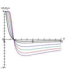
where is an analytic function of , and the equilibrium correlation is given by . In Fig. 2, we plot the equilibrium correlation as a function of the temperature for the parameters and . The bold solid curve denotes the case of the model given by eq. (2). Hereafter, we take as the unit of energy. The temperature is also scaled by .

In Fig. 2, we can observe nonmonotonic temperature dependence. The correlation at the higher-temperature side is small. To increase this amplitude, we provide a multiplied decoration bond with intermediate spins (the open circles depicted in Fig. 1(b)). Therefore, the total number of spins is . The Hamiltonian in this case is given by
| (5) |
and the effective coupling between and is given by
| (6) |
The correlation functions for various values of are also plotted in Fig. 2.
Now we study the dynamics of the correlation function
| (7) |
where is the distribution function at time . We adopt the Glauber-type kinetic Ising model[10] for the time evolution
| (8) |
with the transition probability per unit time
| (9) |
where
| (10) |
It is convenient to use the vector consisting of the probabilities of the states
| (11) |
The dynamics is expressed by
| (12) |
where is a matrix with matrix elements at the small limit of .
| (13) |
and
| (14) |

Hereafter, we adopt eq. (12) as an approximate discrete form of eq. (8). Here, we suddenly change the temperature from to and study the subsequent dynamics by iterating the time evolution operator with . We call an update by this procedure a “Monte Carlo step (MCS)”. The initial probability distribution is set to be the equilibrium one at .
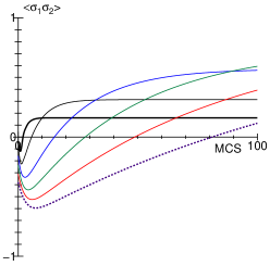
In Fig. 3, we depict the time evolution of the correlation . We find that first decreases, the amplitude increases on the negative side, it then becomes positive, and finally it reaches the equilibrium value at . This observation indicates that even if the temperature is changed suddenly to , the correlation function does not necessarily relax directly toward its new equilibrium value, but it can show nonmonotonic relaxation. We may understand that the “effective temperature” of the system decreases gradually even when the temperature of the thermal bath is changed suddenly. The correlation function, as well as other quantities, shows a similar dependence to its temperature dependence. That is, if a quantity shows a nonmonotonic temperature dependence in equilibrium, it tends to show nonmonotonic relaxation.
To understand this nonmonotonic behavior, we analyze the time evolution from the viewpoint of the eigenvalue problem of the time-evolution operator .[11] Let and be the th right eigenvector of and the eigenvalue, respectively ()
| (15) |
Here, we assume that . The state gives the equilibrium state at . The initial state (the equilibrium state at ) is expanded using as
| (16) |
After time evolutions by , the state evolves to
| (17) |
The contribution of the th mode to the correlation function is
| (18) |
The sign of can be either positive or negative, and the contribution of each mode causes a decrease or increase in corresponding to the sign of . The relaxation time of each mode is different and can be nonmonotonic. Here we demonstrate this situation taking the simplest case of .
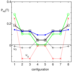
In the case of , there are 8 modes. The eigenvalues and the coefficients are plotted in Fig. 4(a). We take the initial state to be the equilibrium state at , and the contribution from some modes is zero because of the symmetry. For example, modes that are antisymmetric in exchanging sites 1 and 2 do not contribute. In the present case, only two modes and 7 contribute. The changes in and are depicted in Fig. 4(b). The contribution from the 7th mode with a short relaxation time (open diamonds) is positive and it relaxes rapidly. This causes the decrease in in the early stages. On the other hand, the contribution of the slow-relaxing mode () is negative and it causes an increase in to the equilibrium value. For larger , we found similar behavior (not shown).

It is interesting to note the characteristics of the relaxation modes. In Fig. 5, we plot the probability distribution in the phase space of the equilibrium states at , 2, and 10. The configurations denote , , , , , respectively. In configurations 1, 4, 5, and 8, the spins and have the same sign and thus there is a ferromagnetic correlation between and , and the configurations 2, 3, 6, and 7 have an antiferromagnetic correlation. We also plot the eigenvectors and at . There, we find that the fast relaxation mode has large amplitudes at configurations 4 and 5, and the reduction of this mode causes the change from to , where the probabilities of the energetically unfavorable configurations 4 and 5 are reduced, and the antiferromagnetic correlation between and slightly increases. The slow relaxation mode corresponds to the difference between and where the ferromagnetic correlation between and increases. Here we find that the relaxation modes reflect the temperature dependence of the equilibrium state. This fact corresponds to the gradual cooling of the system.
Next, we study the antiferromagnetically coupled spin cluster in a uniform magnetic field
| (19) |
where and are competing. In other words, this system has “frustration” between the magnetic coupling and the magnetic field. In Fig. 6(a), we depict the temperature dependence of the magnetization in the magnetic field . The magnetization shows nonmonotonic behavior as a function of temperature. The temperature is scaled by . The time evolution of after sudden quenching of the temperature from to 0.1 is plotted in Fig. 6(b). Here we again find the same nonmonotonic behavior.
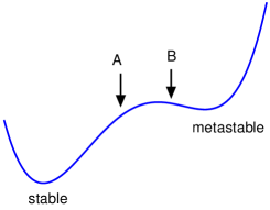
We also refer to nonmonotonic behavior in macroscopic models. If the system has a metastable state that is separated from the equilibrium state by a free energy barrier, as depicted in Fig. 7, the system can show nonmonotonic behavior. For example, if the initial state is point B, it relaxes to the metastable point in a short time, and later it relaxes to the equilibrium state via a nucleation process. This is characteristically different from the simple relaxation starting from point A. Thus, this type of difference in the relaxation has been used to detect a metastable state.[12] In the present macroscopic case, there are also two competing structures representing the metastable state and the equilibrium state.
 |
In the present study, we only investigated the cases with sudden changes in the temperature. It is also interesting to change the temperature with a finite sweep velocity. If we sweep the temperature sufficiently slowly, a quasi-static state should be realized. The sweep velocity dependence of the dynamics will be studied in the near future.
Using a lattice constructed by the decoration bond, we can study the reentrant phase transition.[8, 9] If we change the temperature suddenly from the paramagnetic region to the ferromagnetic region, we obtain very slow relaxation due to an entropy-induced screening effect.[9] Here, we find that the antiferromagnetic correlation appears for only a very short time and the nonmonotonicity does not develop. To achieve nonmonotonic behavior on a macroscopic scale, we have to construct a system where the present mechanics takes place on a coarse-grained scale. Here, the present spin should represent a coarse-grained local magnetization. In spin glasses, the frustrated configuration remains in each step of the coarse-grain magnetization process, which may be called a “hierarchical structure”. Furthermore, in real spin glasses, the spin directions in the ordered configuration are spatially random, and we need to average these over all the possible configurations. Thus, the temperature dependence of the uniform magnetization is averaged out, although the local spin correlations may show various peculiar temperature dependences. However, the hierarchical frustrated structure causes peculiar phenomena in the time dependence. As was proposed by Takayama and Hukushima, the magnetization first decreases while the short-range spin glass correlation still increases, whereas it finally increases after the correlation reaches the saturated value where the local magnetization behaves independently. This complexity causes the peculiar spin glass properties, but the present mechanism may give the basic local mechanism of these phenomena.
We would like to express our thanks to Professor Takayama for the kind explanation of the paper.[1] This work was partially supported by Grant-in-Aid for Scientific Research on Priority Areas “Physics of new quantum phases in superclean materials” (Grant No. 17071011) from MEXT, by the Next Generation Super Computer Project, Nanoscience Program from MEXT, and also by the 21st Century COE Program at the University of Tokyo “Quantum Extreme Systems and Their Symmetries” from the Ministry of Education, Culture, Sports, Science and Technology of Japan. The authors thank the Supercomputer Center, Institute for Solid State Physics, University of Tokyo for the use of the facilities.
References
- [1] H. Takayama and K. Hukushima: J. Phys. Soc. Jpn. 76 (2007) 013702.
- [2] T. Jonsson, K. Jonason, and P. Nordblad: Phys. Rev. B 59 (1999) 9402.
- [3] P. E. Jönsson and H. Takayama: J. Phys. Soc. Jpn 74 (2005) 1131.
- [4] I. Syozi: Phase Transition and Critical Phenomena, Vol. 1, Domb and Green eds. (Academic Press, New York, 1972) p.269.
- [5] S. Miyashita: Prog. Theor. Phys. 69 (1983) 714.
- [6] H. Kitatani, S. Miyashita, and M. Suzuki: J. Phys. Soc. Jpn. 55 (1986) 865.
- [7] M. Jaščur and J. Strečka: Condens. Matter Phys. 8 (2005) 869.
- [8] S. Miyashita and E. Vincent: Eur. Phys. J. B 22 (2001) 203.
- [9] S. Tanaka and S. Miyashita: Prog. Theor. Phys. Suppl. 157 (2005) 34.
- [10] R. J. Glauber: J. Math. Phys., 4 (1963) 294.
- [11] The time evolution function is symmetrized in the form . Here, is the diagonal matrix with . Let be the eigenvectors of , i.e., . The eigenvectors of are given by with the same eigenvalues. Here we must be careful about the normalization of the vector. As the eigenstate of the matrix , the eigenstates are normalized as . On the other hand, the normalization of the probability is given by (*). Although , we need to scale to satisfy the condition (*).
- [12] Y. Konishi, H. Tokoro, M. Nishino, and S. Miyashita: J. Phys. Soc. Jpn. 75 (2006) 114603.