Point process model of 1/f noise versus a sum of Lorentzians

Abstract

To be published in Phys. Rev. E (2005).

We present a simple point process model of $1/f^{\beta}$ noise, covering different values of the exponent $\beta$. The signal of the model consists of pulses or events. The interpulse, interevent, interarrival, recurrence or waiting times of the signal are described by the general Langevin equation with the multiplicative noise and stochastically diffuse in some interval resulting in the power-law distribution. Our model is free from the requirement of a wide distribution of relaxation times and from the power-law forms of the pulses. It contains only one relaxation rate and yields $1/f^{\beta}$ spectra in a wide range of frequency. We obtain explicit expressions for the power spectra and present numerical illustrations of the model. Further we analyze the relation of the point process model of $1/f$ noise with the Bernamont-Surdin-McWhorter model, representing the signals as a sum of the uncorrelated components. We show that the point process model is complementary to the model based on the sum of signals with a wide-range distribution of the relaxation times. In contrast to the Gaussian distribution of the signal intensity of the sum of the uncorrelated components, the point process exhibits asymptotically a power-law distribution of the signal intensity. The developed multiplicative point process model of $1/f^{\beta}$ noise may be used for modeling and analysis of stochastic processes in different systems with the power-law distribution of the intensity of pulsing signals.

I Introduction

$1/f$ fluctuations are widely found in nature, i.e., the power spectra $S(f)$ of a large variety of physical, biological, geophysical, traffic, financial and other systems at low frequencies $f$ have $1/f^{\beta}$ (with $0.5\lesssim\beta\lesssim 1.5$) behavior Press78 ; rev1 ; Thu97 ; Scien95 . Widespread occurrence of signals exhibiting such a behavior suggests that a generic mathematical explanation of $1/f$ noise might exist. The generic origins of two popular noises: white noise (no correlation in time, $S(f)\sim 1/f^{0}$) and Brownian noise (no correlation between increments, $S(f)\sim 1/f^{2}$) are very well known and understood. It should be noted, that the Brownian motion is the integral of white noise and that operation of integration of the signal increases the exponent by 2 while the inverse operation of differentiation decreases it by 2. Therefore, $1/f$ noise can not be obtained by simple procedure of integration or differentiation of such convenient signals. Moreover, there are no simple, even linear stochastic differential equations generating signals with $1/f$ noise. Recently we derive a stochastic nonlinear differential equation for the signal exhibiting $1/f$ noise in any desirably wide range of frequency KR04 . The physical interpretation of this highly nonlinear equation is not so clear and straightforward as that of the linear Langevin equation, generating the Brownian motion of the signal with $1/f^{2}$ spectrum. Therefore, $1/f$ noise is often represented as a sum of independent Lorentzian spectra with a wide range of relaxation times b1 . Summation or integration of the Lorentzians with the appropriate weights may yield $1/f$ noise.

Not long ago a simple analytically solvable model of $1/f$ noise has been proposed Ka98 , analyzed KM98 ; Ka2000 , and generalized KM99 . The signal in the model consists of pulses or series of events (a point process). The interpulse times of the signal stochastically diffuse about some average value. The process may be described by an autoregressive iteration with a very small relaxation. The proposed model reveals one of the possible origins of $1/f$ noise, i.e., random increments of the time interval between the pulses (the Brownian motion in the time axis), sometimes resulting in the clustering of the signal pulses Ka98 ; KM98 ; KM99 .

The power spectral density of such point process may be expressed as

$$S(f)\simeq 2\bar{I}^{2}\bar{\tau}P_{k}\left(0\right)/f.$$ (1)

Here $\bar{\tau}=\left\langle\tau_{k}\right\rangle$ is the expectation of the interpulse time $\tau_{k}=t_{k+1}-$ $t_{k}$, with $\left\{t_{k}\right\}$ being the sequence of the pulses occurrence times or arrival times $t_{k}$, whereas $P_{k}\left(\tau_{k}\right)$ is a steady state distribution density of the interpulse time $\tau_{k}$ in $k$-space and $\bar{I}$ is the average intensity of the signal

$$I\left(t\right)=\sum_{k}A_{k}\left(t-t_{k}\right).$$ (2)

Function $A_{k}\left(t-t_{k}\right)$ represents the shape of the $k$-pulse of the signal in the region of the pulse occurrence time $t_{k}$.

It is easy to show that the fluctuations and shapes of $A_{k}\left(t-t_{k}\right)$ for sharp pulses mainly influence the high frequency power spectral density. Therefore, in a low frequency region we can restrict our analysis to the noise originated from the correlations between the occurrence times $t_{k}$. Then we can simplify the signal to the point process

$$I\left(t\right)=\bar{a}\sum_{k}\delta\left(t-t_{k}\right)$$ (3)

with $\bar{a}$ being an average contribution to the signal of one pulse or one particle when it crosses the section of observation.

Point processes arise in different fields, such as physics, economics, cosmology, ecology, neurology, seismology, traffic flow, signaling and telecom networks, audio streams, and Internet (see, e.g., Thu97 ; Grun ; Earth ; tr ; p1 and references herein). The proposed point process model Ka98 ; KM98 ; KM99 can been modified and useful for the modeling and analysis of self-organized systems p2 , atmospheric variability p3 , large flares from Gamma-ray Repeaters in astronomy p4 , particles moving in viscous fluid p5 , dynamical percolation p6 , $1/f$ noise observed in cortical neurons and earthquake data p7 , financial markets GoKa03 , cognitive experiments Scien95 ; p8 , the Parkinsonian tremors p9 , and time intervals production in tapping and oscillatory motion of the hand HM2004 .

The analytically solvable model and its generalizations Ka98 ; KM98 ; Ka2000 ; KM99 contain, however, some shortage of generality, i.e., it results only in exact $1/f$ (with $\beta=1$) noise and only if $P_{k}\left(\tau_{k}\right)\simeq const$ when $\tau_{k}\rightarrow 0$. On the other hand, the numerical analysis of the generalized model with different restrictions for diffusion of the interpulse time $\tau_{k}$ reveals $1/f^{\beta}$ spectra with $1\lesssim\beta\lesssim 1.5$ KM99 .

The aims of this paper are to generalize the analytical model seeking to define the variety of time series exhibiting the power spectral density $S(f)\sim 1/f^{\beta}$ with $0.5\lesssim\beta\lesssim 2$ and to analyze the relation of the point process model with the Bernamont-Surdin-McWhorter model b1 , representing the signal as a sum of the appropriate signals with the different rates of the linear relaxation.

II Power spectral density of the point process

The point process is primarily and basically defined by the occurrence times $t_{k}$. The power spectral density of the point process (3) may be expressed as Ka98 ; KM98 ; KM99

$$S\left(f\right) = \lim\limits_{T\rightarrow\infty}\left\langle\frac{2}{T}\int\limits_{t_{i}}^{t_{f}}\int\limits_{t_{i}}^{t_{f}}I\left(t^{\prime}\right)I\left(t^{{}^{\prime\prime}}\right)e^{i\omega\left(t^{{}^{\prime\prime}}-t^{\prime}\right)}{\rm d}t^{\prime}{\rm d}t^{{}^{\prime\prime}}\right\rangle$$ (4)

$$= \lim\limits_{T\rightarrow\infty}\left\langle\frac{2\bar{a}^{2}}{T}\left|\sum_{k=k_{\min}}^{k_{\max}}e^{-i\omega t_{k}}\right|^{2}\right\rangle$$

$$= \lim\limits_{T\rightarrow\infty}\left\langle\frac{2\bar{a}^{2}}{T}\sum_{k=k_{\min}}^{k_{\max}}\sum_{q=k_{\min}-k}^{k_{\max}-k}e^{i\omega\Delta\left(k;q\right)}\right\rangle$$

where $T=t_{f}-t_{i}\gg\omega^{-1}$ is the observation time, $\omega=2\pi f$, and

$$\Delta\left(k;q\right)\equiv t_{k+q}-t_{k}=\sum_{i=k}^{k+q-1}\tau_{i}$$ (5)

is the difference between the pulses occurrence times $t_{k+q}$ and $t_{k}$. Here $k_{\min}$ and $k_{\max}$ are minimal and maximal values of index $k$ in the interval of observation $T$ and the brackets $\left\langle...\right\rangle$ denote the averaging over realizations of the process.

It should be stressed that the spectrum is related to the underlying process and not to a realization of the process r1 ; r2 . Therefore, the averaging over realizations of the process is essential. Without the averaging over the realizations we obtain the squared modulus of the Fourier transform of the data, i.e., the periodogram which is fluctuating wildly and its variance is almost independent of $T$ r1 ; r2 . For calculation of the power spectrum of the actual signal without the averaging over the realizations one should use the well-known procedures of the smoothing for spectral estimations r1 ; r2 ; Marpl ; Stoica .

Equation (4) may be rewritten as

$$S\left(f\right)=2\bar{a}^{2}\bar{\nu}+\lim\limits_{T\rightarrow\infty}\left\langle\frac{4\bar{a}^{2}}{T}\sum_{q=1}^{N}\sum_{k=k_{\min}}^{k_{\max}-q}\cos\left[\omega\Delta\left(k;q\right)\right]\right\rangle$$ (6)

where $N=k_{\max}-k_{\min}$ and

$$\bar{\nu}=\frac{1}{\bar{\tau}}=\left\langle\lim\limits_{T\rightarrow\infty}\frac{N+1}{T}\right\rangle$$

is the mean number of pulses per unit time. The first term in the right-hand-site of Eq. (6) represents the shot noise,

$$S_{{\rm shot}}\left(f\right)=2\bar{a}^{2}\bar{\nu}=2\bar{a}\bar{I},$$ (7)

with $\bar{I}=\bar{a}\bar{\nu}$ being the average signal.

Eqs. (4)-(7) may be modified as

$$S\left(f\right)=2\bar{a}^{2}\sum\limits_{q=-N}^{N}\left(\bar{\nu}-\frac{\left|q\right|}{T}\right)\chi_{\Delta\left(q\right)}\left(\omega\right)$$ (8)

and used for evaluation of the power spectral density of the non-stationary process or for the process of finite duration, as well. Here

$$\chi_{\Delta\left(q\right)}\left(\omega\right)=\overline{\left\langle e^{i\omega\Delta\left(q\right)}\right\rangle}=\int\limits_{-\infty}^{+\infty}e^{i\omega\Delta\left(q\right)}\Psi_{q}\left(\Delta\left(q\right)\right)d\Delta\left(q\right)$$ (9)

is the characteristic function of the distribution density $\Psi_{q}\left(\Delta\left(q\right)\right)$ of $\Delta\left(q\right)$, a definition $\Delta\left(q\right)=-\Delta\left(-q\right)=\Delta\left(k;q\right)$ is introduced, and the brackets $\overline{\left\langle\ldots\right\rangle}$ denote the averaging over realizations of the process and over the time (index $k$) KM98 ; KM99 . For the non-stationary process or process of the finite duration one should use the real distribution $\Psi_{q}\left(\Delta\left(q\right)\right)$ with the finite interval of the variation of $\Delta\left(q\right)$ or calculate the power spectra directly according to Eq. (4).

When the second sum of Eq. (8) in the limit $T\rightarrow\infty$, due to the decrease of the characteristic function $\chi_{\Delta\left(q\right)}\left(\omega\right)$ for finite $\omega$ and large $q$, approaches to zero,

$$\lim\limits_{T\rightarrow\infty}\frac{1}{T}\sum\limits_{q=-N}^{N}\left|q\right|\chi_{\Delta\left(q\right)}\left(\omega\right)\rightarrow 0,$$

we have from Eq. (8) the power spectrum in the form

$$S\left(f\right)=\lim\limits_{T\rightarrow\infty}\left\langle\frac{2\bar{a}^{2}}{T}\sum\limits_{k,q}{e}^{i\omega\Delta\left(k;q\right)}\right\rangle=2\bar{I}^{2}\bar{\tau}\sum\limits_{q=-N}^{N}\chi_{\Delta\left(q\right)}\left(\omega\right).$$ (10)

III Stochastic multiplicative point process

According to the above analysis, the power spectrum of the point process signal is completely described by the set of the interpulse intervals $\tau_{k}=t_{k+1}-$ $t_{k}$. Moreover, the low frequency noise is defined by the statistical properties of the signal at large-time-scale, i.e., by the fluctuations of the time difference $\Delta\left(k;q\right)$ at large $q$, determined by the slow dynamics of the average interpulse interval $\tau_{k}\left(q\right)=\Delta\left(k;q\right)/q$ between the occurrence of pulses $k$ and $k+q$. In such a case quite generally the dependence of the interpulse time $\tau_{k}$ on the occurrence number $k$ may be described by the general Langevin equation with the drift coefficient $d\left(\tau_{k}\right)$ and a multiplicative noise $b\left(\tau_{k}\right)\xi\left(k\right)$,

$$\frac{d\tau_{k}}{dk}=d\left(\tau_{k}\right)+b\left(\tau_{k}\right)\xi\left(k\right).$$ (11)

Here we interpret $k$ as continuous variable while the white Gaussian noise $\xi\left(k\right)$ satisfies the standard condition

$$\left\langle\xi\left(k\right)\xi\left(k^{\prime}\right)\right\rangle=\delta\left(k-k^{\prime}\right)$$

with the brackets $\left\langle...\right\rangle$ denoting the averaging over the realizations of the process. Equation (11) we understand in Ito interpretation.

Perturbative solution of Eq. (11) in the vicinity of $\tau_{k}$ yields

$$\tau_{k+j}\simeq\tau_{k}+d\left(\tau_{k}\right)j+b\left(\tau_{k}\right)\int\limits_{k}^{k+j}\xi\left(l\right)dl,$$ (12)

$$\Delta\left(k;q\right)=\sum_{i=k}^{k+q-1}\tau_{i}\simeq\int\limits_{0}^{q}\tau_{k+j}dj\simeq\tau_{k}q+d\left(\tau_{k}\right)\frac{q^{2}}{2}+b\left(\tau_{k}\right)\int\limits_{0}^{q}dj\int\limits_{k}^{k+j}\xi\left(l\right)dl.$$ (13)

After integration by parts we have

$$\Delta\left(k;q\right)=\tau_{k}q+d\left(\tau_{k}\right)\frac{q^{2}}{2}+b\left(\tau_{k}\right)\int\limits_{k}^{k+q}\left(k+q-l\right)\xi\left(l\right)dl,$$ (14)

$$\left\langle\Delta\left(k;q\right)\right\rangle=\tau_{k}q+d\left(\tau_{k}\right)\frac{q^{2}}{2}.$$ (15)

Analogously, in the same approximation we can obtain and the variance $\sigma_{\Delta}^{2}(k;q)=\left\langle\Delta\left(k;q\right)^{2}\right\rangle-\left\langle\Delta\left(k;q\right)\right\rangle^{2}$ of the time difference $\Delta\left(k;q\right)$,

$$\sigma_{\Delta}^{2}(k;q)=b^{2}\left(\tau_{k}\right)\frac{q^{3}}{3}.$$ (16)

III.1 Power spectral density

Substituting Eqs. (14) and (15) into Eq. (10) and replacing the averaging over $k$ by the averaging over the distribution of the interpulse times $\tau_{k}$ we have the power spectrum

$$S\left(f\right) = 4\bar{I}^{2}\bar{\tau}\int\limits_{0}^{\infty}d\tau_{k}P_{k}\left(\tau_{k}\right)\mathop{\mathrm{Re}}\int\limits_{0}^{\infty}dq\exp\left\{i\omega\left[\tau_{k}q+d\left(\tau_{k}\right)\frac{q^{2}}{2}\right]\right\}$$ (17)

$$= 2\bar{I}^{2}\frac{\bar{\tau}}{\sqrt{\pi}f}\int\limits_{0}^{\infty}P_{k}\left(\tau_{k}\right)\mathop{\mathrm{Re}}\left[{e}^{-i\left(x-\frac{\pi}{4}\right)}\mathop{\mathrm{erfc}}\sqrt{-ix}\right]\frac{\sqrt{x}}{\tau_{k}}d\tau_{k}$$

where $x=\pi f\tau_{k}^{2}/d\left(\tau_{k}\right)$.

The replacement of the averaging over $k$ and over realizations of the process by the averaging over the distribution of the interpulse times $\tau_{k}$, $P_{k}\left(\tau_{k}\right)$, is possible when the process is ergodic. Ergodicity is usually a common feature of the stationary process described by the general Langevin equation Gar85 . Therefore, we will consider the stationary processes of diffusion of the interpulse time $\tau_{k}$ described by Eq. (11) and restricted in the finite interval the motion. Such restrictions may be introduced as some additional conditions to the stochastic equation. The similar restrictions, however, may be fulfilled by introducing some additional terms into Eq. (11), corresponding to the diffusion in some “potential well”, as in paper KR04 .

Approach (17) is the improvement of the simplest model of the pure $1/f$ noise Ka98 ; KM98 taking into account the second, drift, term $d\left(\tau_{k}\right)q^{2}/2$ in expression for $\Delta\left(k;q\right)$. Note, that for $d\left(\tau_{k}\right)\rightarrow 0$ from Eq. (17) we recover the known result (1).

According to Eqs. (1), (4) and (17) the small interpulse times and the clustering of the pulses make the greatest contribution to $1/f^{\beta}$ noise. The power-law spectral density is very often related with the power-law behavior of other characteristics of the signal, such as autocorrelation function, probability densities and other statistics, and with the fractality of the signals, in general Thu97 ; b8 ; Mand97 ; Mand99 ; b11 ; Heavy03 ; b10 . Therefore, we investigate the power-law dependences of the drift coefficient and of the distribution density on the time $\tau_{k}$ in some interval of the small interpulse times, i.e.,

$$d\left(\tau_{k}\right)=\gamma\tau_{k}^{\delta},\quad P_{k}\left(\tau_{k}\right)=C\tau_{k}^{\alpha},\quad\tau_{\min}\leq\tau_{k}\leq\tau_{\max}$$ (18)

where the coefficient $\gamma$ represents the rate of the signal’s nonlinear relaxation and $C$ has to be defined from the normalization.

The power-law distribution of the interpulse, interevent, interarrival, recurrence or waiting time is observable in different systems from physics, astronomy and seismology to the Internet, financial markets and neural spikes (see, e.g., Thu97 ; p1 ; p2 ; r3 and references herein).

One of the most direct applications of the model described by Eq. (18), perhaps, is for the modeling of the computer network traffic p1 with the spreading of the packets of the requested files in the Internet traffic and exhibiting the power-law distribution of the inter-packet time. The modeling of these processes is under way.

Because of the divergence of the power-law distribution and requirement of the stationarity of the process the stochastic diffusion may be realized over a certain range of the variable $\tau_{k}$ only. Therefore, we restrict the diffusion of $\tau_{k}$ in the interval $[\tau_{\min},\tau_{\max}]$ with the appropriate boundary conditions. Then the steady state solution of the stationary Fokker-Planck equation with a zero flow corresponding to Eq. (11) is Gar85

$$P_{k}\left(\tau_{k}\right)=\frac{C}{b^{2}\left(\tau_{k}\right)}\exp\left\{2\int\limits_{\tau_{\min}}^{\tau_{k}}\frac{d\left(\tau\right)}{b^{2}\left(\tau\right)}d\tau\right\}.$$ (19)

For the particular power-law coefficients $d\left(\tau_{k}\right)$ and $b\left(\tau_{k}\right)$ (see, e.g., Eq.(26)) we can obtain the power-law stationary distribution density (18).

Then equations (17) and (18) yield the power spectra with different slopes $\beta$, i.e.,

$$S\left(f\right)=\frac{2\bar{I}^{2}}{\sqrt{\pi}\left(2-\delta\right)f}\left(\frac{f_{0}}{f}\right)^{\frac{\alpha}{2-\delta}}I_{\kappa}\left(x_{\min},x_{\max}\right),$$ (20)

$$I_{\kappa}\left(x_{\min},x_{\max}\right)=\mathop{\mathrm{Re}}\int\limits_{x_{\min}}^{x_{\max}}{e}^{-i\left(x-\frac{\pi}{4}\right)}\mathop{\mathrm{erfc}}\left(\sqrt{-ix}\right)x^{\kappa}dx.$$ (21)

Here $\kappa=\frac{\alpha}{2-\delta}-\frac{1}{2}$, $x_{\min}=f/f_{2}$, $x_{\max}=f/f_{1}$,

$$f_{0}=\frac{\gamma}{\pi}\left(C\bar{\tau}\right)^{\frac{2-\delta}{\alpha}},\quad f_{1}=\frac{\gamma}{\pi\tau_{\max}^{2-\delta}},\quad f_{2}=\frac{\gamma}{\pi\tau_{\min}^{2-\delta}}.$$ (22)

Note that $f_{0}$ is indefinite when $\alpha\rightarrow 0$, however, $f_{0}^{\frac{\alpha}{2-\delta}}$ is definite and converges to $C\bar{\tau}$ in this limit.

We note the special cases of the power spectral density (20).

(i) $f_{1}\ll f\ll f_{2}$, $-1<\kappa<1/2$,

$$S\left(f\right)=\frac{\Gamma\left(1+\kappa\right)\bar{I}^{2}}{\sqrt{\pi}\left(2-\delta\right)\cos\left[\left(\kappa/2+1/4\right)\pi\right]f}\left(\frac{f_{0}}{f}\right)^{\kappa+\frac{1}{2}},$$ (23)

i.e., $S\left(f\right)\sim 1/f^{1+\frac{\alpha}{2-\delta}}$ and $S\left(f\right)\sim 1/f$ for $\alpha=0$, in accordance with Eq. (1).

(ii) $f\ll f_{1}$, $\kappa>-1$,

$$S\left(f\right)=\frac{\bar{I}^{2}}{\left(1+\alpha-\delta/2\right)}\left(\frac{f_{0}}{f_{1}}\right)^{\frac{\alpha}{2-\delta}}\sqrt{\frac{2}{\pi f_{1}f}},$$ (24)

i.e., for very low frequencies $S\left(f\right)\sim 1/\sqrt{f}$.

(iii) $f\gg f_{2}$, $\kappa<1/2$,

$$S\left(f\right)=\frac{\bar{I}^{2}}{\sqrt{\pi}\left(2-\alpha-\delta\right)}\left(\frac{f_{0}}{f_{2}}\right)^{\frac{\alpha}{2-\delta}}\frac{f_{2}}{f^{2}},$$ (25)

i.e., for high frequencies $S\left(f\right)\sim 1/f^{2}$.

For very high frequencies $f\gg\tau_{\max}^{-1}$, however, we can not replace the summation in Eq. (10) by the integration. Then from Eqs. (6) or (10) one gets the shot noise $S\left(f\right)=2\bar{a}\bar{I}$, Eq. (7).

Equations (20) and (23)-(25) reveal that the proposed model of the stochastic multiplicative point process may result in the power-law spectra over several decades of low frequencies with the slope $\beta$ between $0.5$ and $2$.

The simplest and well-known process generating the power-law probability distribution function for $\tau_{k}$ is a multiplicative stochastic process with $b\left(\tau_{k}\right)=\sigma\tau_{k}^{\mu}$ and $\delta=2\mu-1$, written as Go02

$$\tau_{k+1}=\tau_{k}+\gamma\tau_{k}^{2\mu-1}+\sigma\tau_{k}^{\mu}\varepsilon_{k}.$$ (26)

Here $\gamma$ represents the relaxation of the signal, while $\tau_{k}$ fluctuates due to the perturbation by normally distributed uncorrelated random variables $\varepsilon_{k}$ with a zero expectation and unit variance and $\sigma$ is a standard deviation of the white noise. According to Eq. (19) the steady state solution of the stationary Fokker-Planck equation with a zero flow, corresponding to Eq. (26), gives the power-law probability density function for $\tau_{k}$ in the $k$-space

$$P_{k}\left(\tau_{k}\right)=\frac{1+\alpha}{\tau_{\max}^{1+\alpha}-\tau_{\min}^{1+\alpha}}\tau_{k}^{\alpha},\quad\alpha=\frac{2\gamma}{\sigma^{2}}-2\mu.$$ (27)

The power spectrum for the intermediate $f$, $f_{1}\ll f\ll f_{2}$, according to Eq. (23) is

$$S(f)=\frac{\left(2+\alpha\right)\left(\beta-1\right)\bar{a}^{2}\Gamma\left(\beta-1/2\right)}{\sqrt{\pi}\alpha\left(\tau_{\max}^{2+\alpha}-\tau_{\min}^{2+\alpha}\right)\sin\left(\pi\ \beta/2\right)}\left(\frac{\gamma}{\pi}\right)^{\beta-1}\frac{1}{f^{\beta}}$$ (28)

where

$$\beta=1+\frac{\alpha}{3-2\mu},\quad\frac{1}{2}<\beta<2.$$ (29)

For $\mu=1$ we have a completely multiplicative point process when the stochastic change of the interpulse time is proportional to itself. Multiplicativity is an essential feature of the financial time series, economics, some natural and physical processes Sa00 .

Another case of interest is with $\mu=1/2$, when the Langevin equation in the actual time takes the form

$$\frac{d\tau}{dt}=\gamma\frac{1}{\tau}+\sigma\xi\left(t\right),$$ (30)

i.e., the Brownian motion of the interpulse time with the linear relaxation of the signal $I\simeq\bar{a}/\tau$.

Figure 1: Power spectral density (4) vs frequency of the signal generated by Eqs. (3) and (26). Numerical simulations are averaged over 10 realizations of $N=10^{6}$ pulse sequences with the parameters $\bar{a}=1$, $\mu=1/2$, $\sigma=0.02$ and different relaxations of the signal $\gamma$. We restrict the diffusion of the interpulse time in the interval $\tau_{\min}=10^{-6}$, $\tau_{\max}=1$ with the reflective boundary condition at $\tau_{\min}$ and transition to the white noise, $\tau_{k+1}=\tau_{\max}+\sigma\varepsilon_{k}$, for $\tau_{k}>\tau_{\max}$. The straight lines represent the analytical results according to Eq. (28).

Figure 2: The same as in Fig. 1 but for $\mu=1$, $\sigma=0.05$ and different parameters $\gamma$.

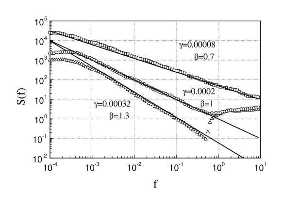
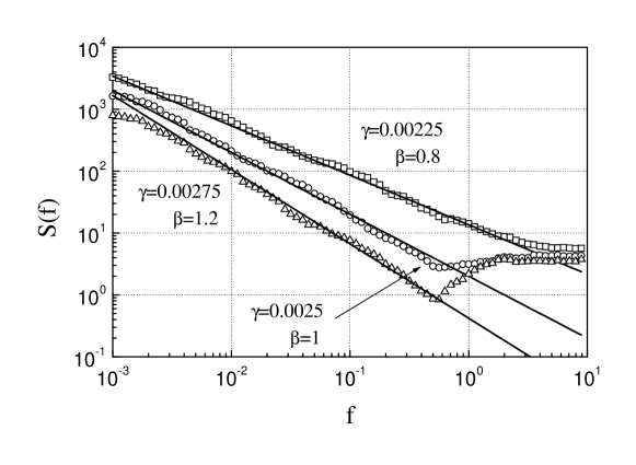
Figures 1 and 2 represent the spectral densities (4) with the different slopes $\beta$ of the signals generated numerically according to Eqs. (3) and (26) for the different parameters of the model. We see that the simple iterative equation (26) with the multiplicative noise produces the signals with the power spectral density of different slopes, depending on the parameters of the model. The agreement of the numerical results with the approximate theory is quite good.

It should be noted that the low frequency noise is insensitive to the small additional fluctuations of the particular occurrence times $t_{k}$. Therefore, we can interpret that Eqs. (11), (26) and (30) describe the slow diffusive motion of the average interpulse time, superimposed by some additional randomness.

On the other hand, the numerical investigations have shown that the proposed model is stable with respect to variation of dynamics of the interpulse time $\tau_{k}$. The substitution of the reflecting boundaries for $\tau_{k}$ by an appropriate confining potential as in Ref. KR04 does not change the result.

III.2 Distribution density of the signal intensity

The origin for appearance of $1/f$ fluctuations in the point process model described by Eqs. (2)-(30) is related with the slow, Brownian fluctuations of the interpulse time $\tau_{k}$ as a function of the pulse number $k$, when the average interpulse time $\tau_{k}(q)$ is a slowly fluctuating function of the arguments $k$ and $q$. In such a case transition from the occurrence number $k$ to the actual time $t$ according to the relation $dt=\tau_{k}dk$ yields the probability distribution density $P_{t}(\tau_{k})$ of $\tau_{k}$ in the actual time $t$,

$$P_{t}(\tau_{k})=P_{k}(\tau_{k})\tau_{k}/\bar{\tau}.$$ (31)

The signal averaged over the time interval $\tau_{k}$ according to Eq. (3) is $I=\bar{a}/\tau_{k}$. Therefore, the distribution density of the intensity of the point process (3) averaged over the time interval $\tau_{k}$ is

$$P(I)=\frac{\bar{a}\bar{I}}{I^{3}}P_{k}\left(\frac{\bar{a}}{I}\right).$$ (32)

If $P_{k}(\tau_{k})\simeq const$ when $\tau_{k}\to 0$ (the condition for the exhibition for the pure $1/f$ noise in the point process model) the distribution density of the signal is

$$P(I)\sim I^{-3}.$$ (33)

For the generalized multiplicative processes (3), (11), and (18) we have from Eqs. (27) and (32) the distribution density of the signal intensity

$$P(I)=\frac{\lambda-1}{\tau_{\max}^{\lambda-1}-\tau_{\min}^{\lambda-1}}\frac{\bar{a}^{\lambda-1}}{I^{\lambda}},\;\lambda=3+\alpha.$$ (34)

The power-law distribution of the signals is observable in a large variety of systems ranging from earthquakes to the financial time series Thu97 ; Earth ; GoKa03 ; b8 ; Mand97 ; Mand99 ; b11 ; Heavy03 ; b10 ; Go02 ; Gop98 .

One of the simplest models generating the Brownian fluctuations of the interpulse time $\tau_{k}$ is an autoregressive model Ka98 ; KM98 ; KM99 with random increments and linear relaxation of the interpulse time, i.e., the model described by the iterative equation

$$\tau_{k+1}=\tau_{k}-\gamma(\tau_{k}-\bar{\tau})+\sigma\varepsilon_{k}.$$ (35)

Here $\bar{\tau}$ is the average interpulse time, $\gamma$ is the rate of the linear relaxation, $\{\varepsilon_{k}\}$ denotes the sequence of uncorrelated normally distributed random variables with zero expectation and a unit variance and $\sigma$ is the standard deviation of this white noise. The model (3), (10), and (35) then results in the power spectral density KM98

$$S(f)=\bar{I}^{2}\frac{\alpha_{H}}{f},\;\alpha_{H}=\frac{2}{\sqrt{\pi}}Ke^{-K^{2}},\;K=\frac{\bar{\tau}\sqrt{\gamma}}{\sigma}.$$ (36)

The distribution density of the intensity of the signal according to Eqs. (19) and (32) then is

$$P(I)=\frac{K\bar{I}^{2}}{\sqrt{\pi}I^{3}}\exp\left\{-\frac{\gamma\bar{a}^{2}}{\sigma^{2}}\left(\frac{1}{\bar{I}}-\frac{1}{I}\right)^{2}\right\}.$$ (37)

Restricting the diffusion of the interpulse time $\tau_{k}$ by the reflective boundary condition at $\tau_{min}>0$ and for $\tau_{min}\to 0$ we have the truncated distribution density of the signal intensity

$$P_{r}(I)=\frac{2K\bar{I}^{2}}{\sqrt{\pi}\left[1+\mathop{\mathrm{erf}}\left(K\right)\right]}\exp\left\{-K^{2}\left(1-\frac{\bar{I}}{I}\right)^{2}\right\}\frac{1}{I^{3}},\;I>0.$$ (38)

In the asymptotic $I\gg\bar{I}$ and $I\gg 2K^{2}\bar{I}$ from Eq. (38) we have

$$P_{r}(I)\simeq\alpha_{H}^{r}\frac{\bar{I}^{2}}{I^{3}}\sim\frac{1}{I^{3}},$$ (39)

i.e., the power-law distribution density of the signal. Here

$$\alpha_{H}^{r}=\frac{\alpha_{H}}{1+\mathop{\mathrm{erf}}\left(K\right)}.$$ (40)

The restriction of motion of $\tau_{k}$ by the reflective boundary condition at $\tau_{k}=0$ reduces the effective (average) value of $P_{k}\left(0\right)=\frac{1}{2}\left[P_{k}\left(\tau_{k}\rightarrow+0\right)+P_{k}\left(\tau_{k}\rightarrow-0\right)\right]$ in Eq. (1) and, consequently, the power spectral density approximately 2 times in comparison with the theoretical result (36) obtained without the restriction, because $P_{k}\left(\tau_{k}\rightarrow-0\right)=0$ for the restricted motion. More exactly, in such a case the power spectral density may be expressed by Eq. (36) with $\alpha_{H}^{r}$ instead of $\alpha_{H}$, i.e.,

$$S_{r}(f)=\bar{I}^{2}\frac{\alpha_{H}^{r}}{f}.$$ (41)

III.3 Correlation function of the point process

Correlation function $C(s)$ of the point process (3) may be expressed as

$$C(s)=\left\langle\frac{\bar{a}^{2}}{T}\sum_{k,q}\delta(t_{k+q}-t_{k}-s)\right\rangle=\bar{I}\bar{a}\sum_{q}\int\limits_{-\infty}^{+\infty}\Psi_{q}\left(\Delta\left(q\right)\right)\delta(\Delta(q)-s)d\Delta\left(q\right)=\bar{I}\bar{a}\sum_{q}\Psi_{q}\left(s\right)$$ (42)

where the brackets $\langle\ldots\rangle$ denote the averaging over the realizations of the process and over time (index $k$) as well. Such averaging coincides with the averaging over the distribution of the time difference $\Delta(q)$, $\Psi_{q}\left(\Delta\left(q\right)\right)$.

From Eq. (42) for the approximation

$$\Delta(k;q)\equiv t_{k+q}-t_{k}=\sum_{l=k+1}^{k+q}\tau_{l}\simeq\tau(q)q,\;q\geq 0$$ (43)

we have the expression for the correlation function in the simplest approximation KM99

$$C(s)\simeq\bar{I}\bar{a}\sum_{q}\int\limits_{\tau_{\min}}^{\tau_{\max}}P_{k}(\tau_{k})\delta(\tau_{k}q-s)d\tau_{k}=\bar{I}\bar{a}\delta(s)+\bar{I}\bar{a}\sum_{q\not=0}P_{k}\left(\frac{s}{q}\right)\frac{1}{|q|}.$$ (44)

Replacing the summation in Eq. (44) by the integration we have the approximate expression for the correlation function of the point processes (3) and (11) or (35)

$$C(s)\simeq\bar{I}\bar{a}\int\limits_{0}^{\infty}P_{k}\left(\frac{s}{q}\right)\frac{dq}{q},\;s\geq 0,\;C(-s)=C(s).$$ (45)

IV Signal as a sum of uncorrelated components

As it was already mentioned above, $1/f$ noise is often modeled as the sum of the Lorentzian spectra with the appropriate weights of a wide range distribution of the relaxation times $\tau^{rel}$. It should be noted that the summation of the spectra is allowed only if the processes with different relaxation times are isolated one from another b1 ; b5 . For the construction of the signal $I(t)$ with $1/f$ noise spectrum from the stochastic equations with a wide range distribution of the relaxation times (and rates $\gamma_{l}=1/\tau^{rel}_{l}$) one should express the signal as a sum of $N$ uncorrelated components Ka2000

$$I(t)=\sum_{l=1}^{N}I_{l}(t)$$ (46)

where every component $I_{l}$ satisfies the stochastic differential equation

$$\dot{I}_{l}=-\gamma_{l}(I_{l}-\bar{I}_{l})+\sigma_{l}\xi_{l}(t).$$ (47)

Here $\bar{I}_{l}$ is the average value of the signal component $I_{l}$ , $\xi_{l}(t)$ is the $\delta$-correlated white noise, $\langle\xi_{l}(t)\xi_{l^{\prime}}(t^{\prime})\rangle=\delta_{l,l^{\prime}}\delta(t-t^{\prime})$, and $\sigma_{l}$ is the intensity (standard deviation) of the white noise.

The distribution density $P(I_{l})$ of the component $I_{l}$ is Gaussian

$$P(I_{l})=\sqrt{\frac{\gamma_{l}}{\pi}}\frac{1}{\sigma_{l}}\exp\left\{-\frac{\gamma_{l}}{\sigma_{l}^{2}}\left(I_{l}-\bar{I}_{l}\right)^{2}\right\}.$$ (48)

The distribution density $P(I)$ of the signal $I(t)$, Eq. (46), expressed as a sum of uncorrelated Gaussian components, is Gaussian as well,

$$P(I)=\frac{1}{\sqrt{2\pi}\sigma}\exp\left\{-\frac{\left(I-\bar{I}\right)^{2}}{2\sigma^{2}}\right\},$$ (49)

with the average value $\bar{I}$ and the variance $\sigma^{2}$ expressed as

$$\bar{I}=\sum_{l}\bar{I}_{l},\;\sigma^{2}=\sum_{l}\frac{\sigma_{l}^{2}}{2\gamma_{l}}.$$ (50)

Therefore, the Bernamont-Surdin-McWhorter model based on the sum of signals with a wide range distribution of the relaxation times always results in the Gaussian distribution of the signal intensity. However, not all signals exhibiting $1/f$ noise are Gaussian rev1 . Some of them are non-Gaussian, exhibiting power-law distribution or even fractal Thu97 ; b8 ; Mand97 ; Mand99 ; b11 ; Heavy03 ; b10 .

Eqs. (46) and (47) result in the expression for the correlation function of the signal (46),

$$C(s)=\sum_{l}\frac{\sigma_{l}^{2}}{2\gamma_{l}}e^{-\gamma_{l}s},\;s\geq 0.$$ (51)

The correlation function (51) yields the power spectrum

$$S(f)=\sum_{l}\frac{2\sigma_{l}^{2}}{\gamma_{l}^{2}+\omega^{2}},\;\omega=2\pi f.$$ (52)

Introducing the distribution of the relaxation rates, $g(\gamma)$, we can replace the summation in Eqs. (46) and (50)-(52) by the integration and express the power spectrum of the signal (46) as

$$S(f)=\int\limits_{\gamma_{\min}}^{\gamma_{\max}}\frac{2\sigma^{2}(\gamma)g(\gamma)}{\gamma^{2}+\omega^{2}}d\gamma=\frac{1}{\pi f}\int\limits_{y_{\min}}^{y_{\max}}\frac{\sigma^{2}(\omega y)g(\omega y)}{1+y^{2}}dy.$$ (53)

Here $\gamma_{\min}$ and $\gamma_{\max}$ are minimal and maximal values of the relaxation rate, respectively.

IV.1 Signals with the pure $1/f$ power spectrum

Eq. (53) yields the pure $1/f$ power spectrum only in the case when $\sigma^{2}(\omega y)g(\omega y)=A=const$. In such a case the correlation function (51) may be expressed as

$$C(s)=\frac{A}{2}\int\limits_{\gamma_{\min}}^{\gamma_{\max}}e^{-\gamma s}\frac{d\gamma}{\gamma}=\frac{A}{2}\int\limits_{\tau_{\min}^{rel}}^{\tau_{\max}^{rel}}e^{-s/\tau^{rel}}\frac{d\tau^{rel}}{\tau^{rel}}$$ (54)

while the power spectrum (53) yields

$$S(f)=\frac{A}{\pi f}\left[\arctan\left(\frac{\gamma_{\max}}{\omega}\right)-\arctan\left(\frac{\gamma_{\min}}{\omega}\right)\right]\simeq\frac{A}{2f},\;\gamma_{\min}\ll\omega\ll\gamma_{\max}.$$ (55)

For the signal expressed not as a sum (46) but as an average of $N$ uncorrelated components,

$$I_{a}(t)=\frac{1}{N}\sum_{l=1}^{N}I_{l}(t),$$ (56)

all characteristics (48)-(55) are similar, except that the average value $\bar{I_{a}}$ of the averaged signal (56) is $N$ times smaller than that according to Eq. (50), while the expressions for the correlation function $C(s)$, Eqs. (51) and (54), for the power spectrum $S(f)$, Eqs. (52), (53), and (55), and for the variance $\sigma_{a}^{2}$, Eq. (50), should be divided by $N^{2}$, i.e.,

$$\bar{I_{a}}=\frac{1}{N}\sum_{l}\bar{I}_{l},\;\sigma_{a}^{2}=\frac{1}{N^{2}}\sum_{l}\frac{\sigma_{l}^{2}}{2\gamma_{l}},$$ (57)

$$S_{a}(f)\simeq\frac{A}{2N^{2}f},$$ (58)

$$C_{a}(s)=\frac{1}{2N^{2}}\int\limits_{\gamma_{\min}}^{\gamma_{\max}}\frac{e^{-\gamma s}}{\gamma}{\sigma^{2}\left(\gamma\right)}g(\gamma)d\gamma.$$ (59)

When replacing the summation in Eqs. (46), (50)-(53) and (56)-(59) by the integration, the distribution density of the relaxation rates, $g\left(\gamma\right)$, should be normalized to the number of uncorrelated components $N$,

$$\int\limits_{\gamma_{\min}}^{\gamma_{\max}}g(\gamma)d\gamma=N.$$ (60)

We see the similarity of expressions (45) and (59) for the correlation function of the point process model and that of the sum of signals with different relaxation rates, respectively. In general, however, different distributions $P_{k}(\tau_{k})$ of the interpulse time $\tau_{k}$ when $P_{k}(0)\not=0$, e.g., exponential, Gaussian and continuous distributions, with the slowly fluctuating interpulse time $\tau_{k}$ may result in $1/f$ noise. Therefore, the point process model is, in some sense, more general than the model based on the sum of the Lorentzian spectra.

Figure 3: Power spectra: (a) numerically calculated for the average signal (56) from $N=10$ components (47) with $\bar{I}=20$, $\sigma_{l}^{2}(\gamma_{l})g(\gamma_{l})=const$ and uniform distribution of $\lg\gamma_{l}$ of $\gamma_{l}$ values in the interval $10^{-4}-10^{0}$, i.e., with $g\left(\gamma_{l}\right)\sim\gamma_{l}^{-1}$, $\sigma^{2}_{l}\left(\gamma_{l}\right)\sim\gamma_{l}$, and $\sigma_{1}\left(\gamma_{1}\right)=0.1$, open circles, in comparison with theoretical results (58), straight line; (b) for the point process (3), (4), and (35) with $\bar{a}=1$, $\bar{\tau}=1$, $\sigma=0.01$, and $\gamma=0.0001$ averaged over 10 realizations of $10^{5}$ pulse sequences, open circles, in comparison with the theoretical results according to Eq. (41), straight line. (c) and (d) numerically calculated distribution densities of the corresponding signals, open circles, in comparison with the theoretical results (49), (57), and (38), solid lines, respectively.

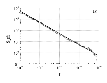
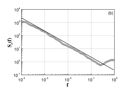
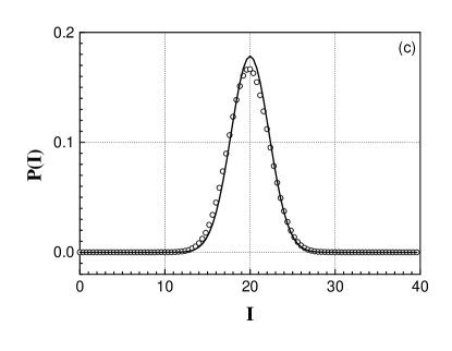
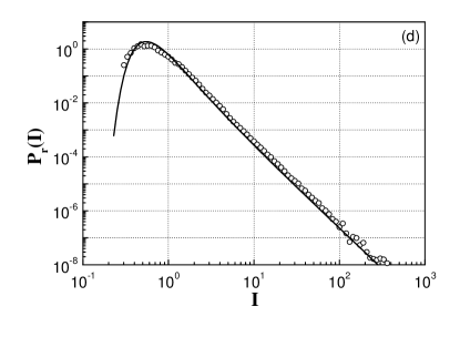
In Figure 3 the examples of the pure $1/f$ power spectra for the average (56) of signals (47) generated for different relaxation rates $\gamma_{l}$ and with the corresponding intensities of the white noise $\sigma_{l}^{2}$ and those of the autoregressive point process (3), (4), and (35) are presented together with the distribution densities of the corresponding signals. We see the similarity of the spectra but very different distributions of the intensity of the signals: the signal of the sum of the Lorentzians is Gaussian while that of the point process is approximately of the power-law type, asymptotically $P(I)\sim I^{-3}$.

IV.2 Signals with the power spectral density of different slopes $\beta$

Using the sum of different Lorentzian signals we can generate not only a signal with the pure $1/f$ spectrum but the signal with any predefined slope $\beta$ of $1/f^{\beta}$ power spectral density, as well. Indeed, let us investigate the case when

$$\sigma^{2}(\gamma)g(\gamma)=A\gamma^{\eta},$$ (61)

where $A$ and $\eta$ are some parameters. Substitution of Eq. (61) into Eq. (53) yields the power spectral density

$$S(f)=\frac{A}{\pi f}\int\limits_{\gamma_{\min}/\omega}^{\gamma_{\max}/\omega}\frac{(\omega y)^{\eta}}{1+y^{2}}dy\\ =\frac{A}{\omega^{1-\eta}}\left\{\left[\frac{\gamma_{\max}}{\omega}\right]^{\eta+1}\Phi\left(-\left[\frac{\gamma_{\max}}{\omega}\right]^{2},1,\frac{\eta+1}{2}\right)\right.\\ \left.-\left[\frac{\gamma_{\min}}{\omega}\right]^{\eta+1}\Phi\left(-\left[\frac{\gamma_{\min}}{\omega}\right]^{2},1,\frac{\eta+1}{2}\right)\right\}$$ (62)

where $\Phi(z,s,a)$ is a Lerch’s Phi transcendent. In the limit when $\gamma_{\min}\to 0$ and $\gamma_{\max}\to\infty$ we can approximate the power spectral density (62) as

$$S(f)\simeq\frac{\left(2\pi\right)^{\eta}A}{2\cos\left(\pi\eta/2\right)}\frac{1}{f^{1-\eta}},$$ (63)

i.e., we have the generalization of the result (55).

For the average signal (56) we have

$$S_{a}(f)\simeq\frac{\left(2\pi\right)^{\eta}A}{2N^{2}\cos\left(\pi\eta/2\right)}\frac{1}{f^{1-\eta}}.$$ (64)

In order to obtain an arbitrary $\beta$ of the $1/f^{\beta}$ power spectral density we should choose in Eq. (61) $\eta=1-\beta$.

The distribution density $P_{a}(I_{a})$ of the average signal $I_{a}(t)$ is Gaussian

$$P_{a}(I_{a})=\frac{1}{\sqrt{2\pi}\sigma_{a}}e^{-\frac{(I-\bar{I}_{a})^{2}}{2\sigma^{2}_{a}}}$$ (65)

with the variance $\sigma_{a}^{2}$ expressed as

$$\sigma_{a}^{2}=\frac{1}{2N^{2}}\int\limits_{\gamma_{\min}}^{\gamma_{\max}}\frac{\sigma^{2}(\gamma)g(\gamma)}{\gamma}d\gamma=\frac{A\left(\gamma_{\max}^{\eta}-\gamma_{\min}^{\eta}\right)}{2N^{2}\eta}.$$ (66)

The correlation function in such a case according to Eq. (59) is

$$C_{a}(s)=\frac{A}{2N^{2}}\int\limits_{\gamma_{\min}}^{\gamma_{\max}}e^{-\gamma s}\gamma^{\eta-1}d\gamma=\frac{A}{2N^{2}s^{\eta}}\left[\Gamma\left(\eta,\gamma_{\min}s\right)-\Gamma\left(\eta,\gamma_{\max}s\right)\right]$$ (67)

where $\Gamma\left(a,z\right)$ is the incomplete gamma function.

Figure 4: Power spectra: (a) numerically calculated for signal (47), (56) and (61) from 10 components with $\bar{I}=20$, $A=100$, $\eta=-0.25$, open circles, and $\eta=0.25$, open squares, in comparison with theoretical results (64), straight line; (b) for the point process (3), (4) and (26) with the parameters $\bar{a}=1$, $\mu=0.5$, $\sigma=0.02$, and $\gamma=0.0001$, open squares, and $\gamma=0.0003$, open circles, averaged over 10 realizations of $10^{6}$ pulse sequences in comparison with the theoretical results (28), straight lines. (c) and (d) numerically calculated distribution densities of the corresponding signals in comparison with the theoretical results (65), (66), and (34), respectively, solid lines.

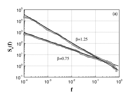
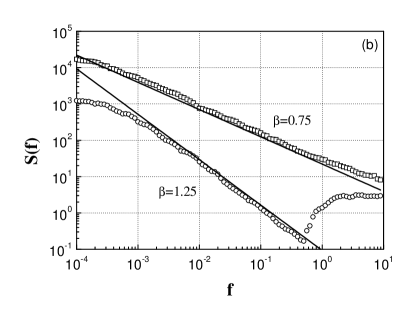
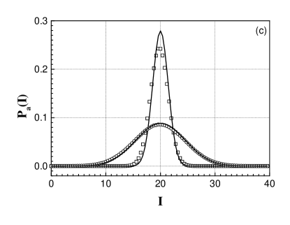
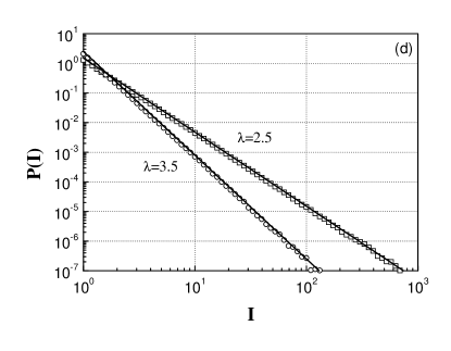
Figure 4 demonstrates the possibility to generate stochastic signals exhibiting similar $1/f^{\beta}$ power spectral densities with different slopes $\beta$ by the summation of signals with different relaxation rates and according to the multiplicative point process model. The distribution densities of the corresponding signals are, however, completely different.

V Conclusions

The generalized multiplicative point processes (3), (11), (18), and (26) may generate time series exhibiting the power spectral density $S(f)\sim 1/f^{\beta}$ with $0.5\lesssim\beta\lesssim 2$, Eqs. (17), (23), and (28), i.e., with the slope observable in a large variety of systems. Such spectral density is caused by the stochastic diffusion of the interpulse time, resulting in the power-law distribution. The power-law distribution of the interpulse, interevent, interarrival, recurrence or waiting times is observed in different systems from physics, astronomy and seismology to the Internet, financial markets, neural spikes, and human cognition.

Furthermore, the power-law distribution of the interpulse time results in the power-law distribution of the stochastic signal, $P(I)\sim I^{-\lambda}$ with $2\lesssim\lambda\lesssim 4$, i.e., the phenomenon observable in a large variety of processes, from earthquakes to the financial time series, as well. The proposed model relates and connects the power-law autocorrelation and spectral density with the power-law distribution of the signal intensity into the consistent theoretical approach. The generated time series of the model are fractal since they exhibit jointly the power-law probability distribution and the power-law autocorrelation of the signal.

In addition, we have analyzed the relation of the point process model with the Bernamont-Surdin-McWhorter model of $1/f$ noise, representing the signal as a sum of the appropriate signals with the different rates of the linear relaxation. From the performed analysis we can conclude that the multiplicative point process model of $1/f$ noise when the signal consisting of pulses with a stochastic motion of the interpulse time is more general and complementary to the model based on the sum of signals with a wide-range distribution of the relaxation times. In contrast to the Gaussian distribution of the intensity of sum of the uncorrelated components, the point process model generating $1/f$ noise exhibits the power-law distribution of the intensity of the signal. Moreover, it is free from the requirement of a wide-range distribution of the relaxation times. Obviously, the multiplicative point process model of $1/f^{\beta}$ noise may be used for modeling and analysis of stochastic processes in different systems exhibiting the pulsing signals.

Acknowledgments

We acknowledge support by the Lithuanian State and Studies Foundation.

References

- (1) J. B. Johnson, Phys. Rev. 26, 71 (1925); W. Schottky, Phys. Rev. 28, 74 (1926); D. W. Allan, Proc. IEEE 54, 221 (1966); C. W. J. Granger, Econometrica 34, 150 (1966); R. F. Voss and J. Clarke, Nature (London) 258, 317 (1975); W. H. Press, Comments Astrophys. 7, 103 (1978); M. Gardner, Sci Am. 238, 16 (1978); A. Lawrence, M. G. Watson, K. A. Pounds, and M. Elvis, Nature (London) 325, 694 (1987).
- (2) F. N. Hooge, T. G. M. Kleinpenning and L. K. J. Vadamme, Rep. Prog. Phys. 44, 479 (1981); P. Dutta and P. M. Horn, Rev. Mod. Phys. 53, 497 (1981); S. M. Kogan, Usp. Fiz. Nauk 145, 285 (1985) [Sov. Phys. Usp. 28, 170 (1985)]; M. B. Weissman, Rev. Mod. Phys. 60, 537 (1988); C. M. Van Vliet, Solid State Electron. 34, 1 (1991); G. P. Zhigal’skii, Usp. Fiz. Nauk 167, 623 (1997) [Phys.-Usp. 40, 599 (1997)]; E. Milotti, arXiv: physics/0204033 (2002); H. Wong, Microel. Reliab. 43, 585 (2003).
- (3) S. Thurner, S. B. Lowen, M. C. Feurstein, C. Heneghan, H. G. Feichtinger, and M. C. Teich, Fractals 5, 565 (1997).
- (4) D. L. Gilden, T. Thornton, and M. W. Mallon, Science 267, 1837 (1995).
- (5) B. Kaulakys and J. Ruseckas, Phys. Rev. E 70, 020101(R) (2004); cond-mat/0408507.
- (6) J. Bernamont, Ann. Physik 7, 71 (1937); M. Surdin, J. Phys. Radium (Serie 7) 10, 188 (1939); F. K. du Pré, Phys. Rev. 78, 615 (1950); A. Van der Ziel, Physica 16, 359 (1950); A. L. McWhorter, in Semiconductor Surface Physics, ed. R. H. Kingston, (University of Pennsylvania, Philadelphia, 1957), p. 207; V. Palenskis, Lit. Fiz. Sb. 30, 107 (1990) [Lith. Phys. J. 30(2), 1 (1990)]; F. N. Hooge, in Proc. 14th Int. Conf. on Noise in Physical Systems and 1/f Fluctuations, Leuven, Belgium, 14-18 July 1997, edited by C. Claeys and E. Simoen (World Scientific, Singapore, 1997), p. 3.
- (7) B. Kaulakys, arXiv: adap-org/9806004 (1998).
- (8) B. Kaulakys and T. Meškauskas, Phys. Rev. E 58, 7013 (1998); adap-org/9812003; B. Kaulakys, Phys. Lett. A 257, 37 (1999); adap-org/9907008.
- (9) B. Kaulakys, Lith. J. Phys. 40, 281 (2000).
- (10) B. Kaulakys and T. Meškauskas, Nonlin. Anal.: Mod. Contr. (Vilnius) 4, 87 (1999); B. Kaulakys and T. Meškauskas, Microel. Reliab. 40, 1781 (2000); cond-mat/0303603; B. Kaulakys, Microel. Reliab. 40, 1787 (2000); cond-mat/0305067.
- (11) K. L. Schick and A. A. Verveen, Nature (London) 251, 599 (1974); F. Gruneis, Physica A 123, 149 (1984); F. Gruneis and H.-J. Baiter, Physica A 136, 432 (1986); F. Gruneis and T. Musha, Jpn. J. Appl. Phys. 25, 1504 (1986); T. Musha, Jpn. J. Appl. Phys. 26, 2022 (1987); F. Gruneis, M. Nakao, and M. Yamamoto, Biolog. Cybern. 62, 407 (1990); F. Gruneis, M. Nakao, Y. Mizutani, M. Yamamoto, M. Meesmann, and T. Musha, Biolog. Cybern. 68, 193 (1993); F. Gruneis, Fluct. Noise Lett. 1, R119 (2001); F. Gruneis, Fluct. Noise Lett. 4, L413 (2004).
- (12) H. R. Bittner, P. Tosi, C. Braun, M. Meesmann, and K. D. Kniffki, Geolog. Rundschau 85, 110 (1996); R. Console and M. Murru, J. Geophys. Res. 106, 8699 (2001); L. Telesca, V. Cuomo, and V. Lapenna, Fluct. Noise Lett. 2, L357 (2002); J. M. Halley and P. Inchausti, Fluct. Noise Lett. 4, R1 (2004); M. Lindman, K. Jonsdottir, R. Roberts, B. Lund, and R. Bodvarsson, Phys. Rev. Lett. 94, 108501 (2005).
- (13) T. Musha and H. Higuchi, Jap. J. Appl. Phys. 15, 1271 (1976); X. Zhang, G. Hu, Phys. Rev. E 52, 4664 (1995); M.Y. Choi and H.Y. Lee , Phys. Rev. E 52, 5979 (1995).
- (14) I. Csabai, J. Phys. A 27, L417 (1994); W. Willinger, M. S. Taqqu, R. Sherman, and D. V. Wilson, IEEE/ACM Trans. Networking, 5, 71 (1997); I. Kaj and I. Marsh, In: Quality of Service in Multiservice IP Networks, ed. M. Ajmone Marsan, G. Corazza. M. Listanti, A. Roveri (Springer-Verlag, Heidelberg, 2003), Lecture Notes in Computer Science 2601, p. 35; A. J. Field, U. Harder, and P. G. Harrison, IEE Proceedings-Communications 151, 355 (2004); S. Cohen, M. S. Taqqu, Methodol. Comput. Appl. Probabil. 6 363 (2004); L. A. N. Amaral, A. Diaz-Guilera, A. A. Moreira, A. L. Goldberger, and L. A. Lipsitz, Proc. Natl. Acad. Sci. USA 101, 15551 (2004).
- (15) J. Davidsen and H. G. Schuster, Phys. Rev. E 62, 6111 (2000); J. Davidsen and M. Paczuski, Phys. Rev. E 66, 050101(R) (2002); Y. Kamitani, H. Suyari, and I. Matsuba, Electron. Communic. Jap. Pt.III 87, 72 (2004).
- (16) J. I. Yano, K. Fraedrich, and R. Blender, J. Climate 14, 3608 (2001); W Muller, R. Blender, and K. Fraedrich, Nonlin. Process. Geophys. 9, 37 (2002); W. W. Tung, M. W. Moncrieff, and J. B. Gao, J. Climate 17, 2736 (2004); J. I. Yano, R. Blender, C. D. Zhang, and K. Fraedrich, Quart. J. Royal Meteor. Soc. 130, 1697 (2004); K. Fraedrich, U. Luksch, and R. Blender, Phys. Rev. E 70, 037301 (2004).
- (17) C. Guidorzi, F. Frontera, E. Montanari, M. Feroci, L. Amati, E. Costa, and M. Orlandini, Astron. Astrophys. 416, 297 (2004).
- (18) M. Agu, H. Akabane, and T. Saito, J. Phys. Soc. Jap. 70, 2798 (2001).
- (19) M. Celasco and R. Eggenhoffner, Eur. Phys. J. 23, 415 (2001).
- (20) J. Davidsen and H. G. Schuster, Phys. Rev. E 65, 026120 (2002).
- (21) V. Gontis, Lith. J. Phys. 41, 551 (2001); arXiv: cond-mat/0201514 (2002); V. Gontis and B. Kaulakys, Proc. 17th Intern. Conf. on Noise and Fluctuations, edited by J. Sikula (Prague, August 18-22, 2003) p. 622; V. Gontis, B. Kaulakys, M. Alaburda, and J. Ruseckas, Sol. St. Phenom. 97-98, 65 (2004); V. Gontis and B. Kaulakys, Physica A 343, 505 (2004); cond-mat/0303089; V. Gontis and B. Kaulakys, Physica A 344, 128 (2004); cond-mat/0412723.
- (22) A. Coza and V. V. Morariu, Physica A 320, 449 (2003); E. -J. Wagenmakers, S. Farrell, and R. Ratcliff, Psychonomic Bulletin & Review 11, 579 (2004).
- (23) J. B. Gao, Medic. & Biolog. Engineer. & Comput. 42, 345 (2004).
- (24) D. Delignieres, L. Lemoine, and K. Torre, Human Movement Science 23, 87 (2004).
- (25) M. B. Priestley, Spectral Analysis and Time Series (Academic Press, San Diego, 1981).
- (26) J. Timmer and M. Konig, Astron. Astrophys. 300, 707 (1995).
- (27) S. L. Marpl, Jr., Digital Spectral Analysis with Applications (Prentice-Hall, New Jersey, 1987).
- (28) P. Stoica and R. L. Moses, Introduction to Spectral Analysis (Prentice-Hall, New Jersey, 1997).
- (29) C.W. Gardiner, Handbook of Stochastic Methods for Physics, Chemistry and Natural Sciences (Springer-Verlag, Berlin, 1985).
- (30) B. B. Mandelbrot, J. Business 36, 394 (1963); I. McHardy and B. Czerny, Nature (London) 325, 696 (1987); G. W. Wornell, Proc. IEEE 81, 1428 (1993); H. Scher, G. Margolin, R. Metzler, J. Klafter, and B. Berkowitz, Geophys. Res. Lett. 29, 1061 (2002); P. Bak, K. Christensen, L. Danon, and T. Scanlon, Phys. Rev. Lett. 88, 178501 (2002); L. Giraitis, P. Kokoszka, R. Leipus, and G. Teyssiere, Acta Applicandae Mathematicae 78, 285 (2003).
- (31) B. B. Mandelbrot, Fractals and Scaling in Finance (Springer, New York 1997).
- (32) B. B. Mandelbrot, Multifractals and Noise: Wild Self-Affinity in Physics (Springer, New York 1999).
- (33) R. N. Mantegna, H. E. Stanley, An Introduction to Econophysics: Correlations and Complexity in Finance (Cambridge University Press, Cambridge, 2000).
- (34) S. T. Rachev (Editor), Handbook of Heavy Tailed Distributions in Finance (Elsevier B.V., 2003).
- (35) X. Gabaix, P. Gopikrishnan, V. Plerou, and E. Stanley, Nature (London) 423, 267 (2003).
- (36) S. B. Lowen and M. C. Teich, IEEE Trans. Inform. Theory 39, 1669 (1993); M. Usher, M. Stemmler, and Z. Olami, Phys. Rev. Lett. 74, 326 (1995); M. Takayasu, H. Takayasu, and T. Sato, Physica A 233, 824 (1996); M. S. Wheatland, Astrophys. J. 536, L109 (2000); J. W. Kirchner, X. Feng, and C. Neal, Nature (London) 403, 524 (2000); E. Scalas, Physica A 287, 468 (2000); F. Lepreti, V. Carbone, and P. Veltri, Astrophys. J. 555, L133 (2001); P. Richmond, Eur. Phys. J. 20, 523 (2001); L. Sabatelli, S. Keating, J. Dudley, and P. Richmond, Eur. Phys. J. 27, 273 (2002); A. Erramilli, M. Roughan, D. Veitch, W. Willinger, Proc. IEEE 90, 800 (2002); S. Abe and N. Suzuki, Eurohys. Lett. 61, 852 (2003); P. L. Conti, A. Lijoi, and F. Ruggeri, Appl. Stochastic Models Bus. Ind. 20, 305 (2004); F. Selcuk, Physica A 333, 306 (2004); T. Kaizoji and M. Kaizoji, Physica A 336, 563 (2004); A. Corral, Phys. Rev. Lett. 92, 108501 (2004); A.-H. Sato, Phys. Rev. E 69, 047101 (2004); M. E. J. Newman, arXiv: cond-mat/0412004; S. M. D. Queiros, C. Anteneodo, C. Tsallis, arXiv: physics/0503024.
- (37) V. Gontis, Nonlin. Anal.: Mod. Contr. (Vilnius) 7, 43 (2002); arXiv: cond-mat/0211317 (2002).
- (38) A.-H. Sato, H. Takayasu, and Y. Sawada, Phys. Rev. E 61, 1081 (2000); Z. F. Huang and S. Solomon, Physica A 306, 412 (2002).
- (39) P. Gopikrishnan, M. Meyer, L. A. N. Amaral, and H. E. Stanley, Eur. Phys. J. B 3, 139 (1998); W. J. Reed and B. D. Hughes, Phys. Rev. E 66, 067103 (2002); N. Scafetta and B. J. West, Phys. Rev. Lett. 92, 138501 (2004); C. B. Yang, J. Phys. A: Math. Gen. 37, L523 (2004); L. A. N. Amaral, D. J. B. Soares, L. R. da Silva, L. S. Lucena, M. Saito, H. Kumano, N. Aoyagi, and Y. Yamamoto, Europhys. Lett. 66, 448 (2004); A. Fujihara, T. Ohtsuki, and H. Yamamoto, Phys. Rev. E 70, 031106 (2004).
- (40) F. N. Hooge, IEEE Trans. Electron. Dev. 41, 1926 (1994); F. N. Hooge, Physica B 239, 223 (1997).