Comment on “Hausdorff Dimension of Critical Fluctuations in Abelian Gauge Theories”

In their Letter Hove , Hove, Mo, and Sudbø derive a simple connection between the anomalous scaling dimension, $\eta$, of the U(1) universality class order parameter, $\phi({\bf x})$, and the Hausdorff dimension, $D_{H}$, of critical loops:

$$\eta+D_{H}=2\;.$$ (1)

In the loop representation, the correlator $G({\bf r})=\langle\phi({\bf r})\phi^{*}(0)\rangle\,\propto\,r^{-(d-2+\eta)}$ describes the distribution of the end-points in open loops. For definiteness, one may think of the high-temperature-expansion loops for the lattice $|\phi|^{4}$-model.

The analysis of Ref. Hove might seem absolutely compelling, being just a translation of the hyperscaling hypothesis into the loop language: At the critical point there should be about one loop of diameter $r$ per volume element $r^{d}$ Williams . Nevertheless, given the result $\eta=0.0380(4)$ of Ref. Campostrini , the relation (1) is in strong contradiction with the value $D_{H}=1.7655(20)$ which we obtained for the 3D $|\phi|^{4}$-model with suppressed leading corrections to scaling Campostrini (and also—with a bit less accuracy—for the standard bond-current model Wallin , and its special version with excluded loop overlaps and self-crossings). The simulations were done with the Worm algorithm Worm .

The hidden flaw in the treatment of Ref. Hove is as follows. When introducing the self-similar expression

$$P({\bf r};N)\;\propto\;N^{-\rho}\,F(r/N^{\Delta})\;,~{}~{}~{}\Delta=1/D_{H}\;$$ (2)

for the probability to find the ends of an open loop of length $N$ being distance ${\bf r}$ away from each other, which is then used to establish the connection between the open and closed loops, the authors take for granted that $F(0)$ is finite. While looking innocent, this is an arbitrary assumption, since the self-similar form (2) is valid only for $r\gg a$, where $a$ is a microscopic cutoff (e.g., the lattice period). Strictly speaking, a closed loop of length $N$ corresponds to $F(a/N^{\Delta})$ rather than to $F(0)$, and one has to work with the generic asymptotic form

$$F(x)\,\propto\,x^{\theta}~{}~{}~{}~{}~{}\mbox{at}~{}~{}~{}~{}~{}x\ll 1\;,$$ (3)

with some exponent $\theta$. With Eq. (3), the hyperscaling argument yields $\rho=(d-\theta)/D_{H}$, and from $G(r)\propto\int dNP({\bf r};N)$ one then obtains

$$\eta+D_{H}=2-\theta\;.$$ (4)

Using high-precision data for $\eta$ and $D_{H}$ mentioned above, we find $\theta=0.1965(20)$.

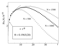
It is instructive to explicitly verify Eq. (3) by simulating $P(r;N)$. In Fig. 1 we present results of such a simulation for the $|\phi|^{4}$-model. We plot the value of $P(r,N)N^{d\Delta}$ as a function of $r$ for three different values of $N$. In view of the self-similarity of $P(r,N)$, the qualitative difference between the cases of $\theta\neq 0$ and $\theta=0$ is readily seen. In the former case, curves for different values of $N$ should merge for $r/N^{\Delta}\ll 1$—and they do in Fig. 1. In the latter case, as $r\to 0$ one should see a fan of curves with essentially different slopes and a common origin at $r=0$.

Figure 1: Distribution of open loops over radii for three different values of $N$. The Worm algorithm simulation Worm was done for the loop representation (high-temperature expansion) of the 3D lattice $|\phi|^{4}$-model with $L=192^{3}$ sites at the special critical point with suppressed leading corrections to scaling Campostrini .

One important implication of Eq. (4) in the absence of additional relation between $D_{H}$, $\eta$ and $\theta$, is that the anomalous scaling dimension can not be deduced from simulations of closed loops which determine $D_{H}$ only.

We are grateful to A. Kuklov, Z. Tešanović, and G. Williams for numerous discussions. This work was supported by the National Science Foundation under Grant DMR-0071767.
Nikolay Prokof’ev and Boris Svistunov,
Department of Physics, University of Massachusetts, Amherst, MA 01003.

PACS numbers: 05.70.Jk, 64.60.Ak, 05.70.Fh

References

- (1) J. Hove, S. Mo, and A. Sudbø, Phys. Rev. Lett. 85, 2368 (2000).
- (2) G.A. Williams, Phys. Rev. Lett. 82, 1201 (1999).
- (3) M. Campostrini et al., Phys. Rev. B, 63, 214503 (2001).
- (4) M. Wallin et al., Phys. Rev. B 49, 12115 (1994).
- (5) N. Prokof’ev and B. Svistunov, Phys. Rev. Lett. 87, 160601 (2001).