Noise activated granular dynamics

Abstract

We study the behavior of two particles moving in a bistable potential, colliding inelastically with each other and driven by a stochastic heat bath. The system has the tendency to clusterize, placing the particles in the same well at low drivings, and to fill all of the available space at high temperatures. We show that the hopping over the potential barrier occurs following the Arrhenius rate, where the heat bath temperature is replaced by the granular temperature. Moreover, within the clusterized “phase” one encounters two different scenarios: for moderate inelasticity, the jumps from one well to the other involve one particle at a time, whereas for strong inelasticity the two particles hop simultaneously.

Granular gases gases , i.e. assemblies of inelastic particles losing a little kinetic energy at each collision, exhibit a variety of complex behaviors, such as clustering goldhirsch , spontaneous formation of vortices bal , lack of energy equipartition Ioepug , non-Maxwellian velocity distributions Nogauss , and so on, which provide new challenges to statistical mechanics. Analogies between standard condensed matter and granular matter remain a valuable route to improve our knowledge of the latter jaeger . As an instance, we mention the analogy between the granular temperature, $T_{G}$, defined as the average kinetic energy per grain, and the temperature of molecular gases. It has been observed that the equality of the granular temperatures of two granular gases is not the condition for thermal equilibrium between them Ioepug . This is not too surprising since it reflects the non-equilibrium nature of granular systems. Nevertheless, one can ask whether $T_{G}$ possesses other useful properties of the thermodynamic temperature, such as that of controlling the rates of activated processes and the direction of energy fluxes. The answer is relevant in the construction of the hydrodynamics of granular systems.

The present work is inspired by the experiment probing the behavior of vibrated sand in a vertical box made up of two identical compartments communicating through a small orifice located at a certain height. One observes that for vigorous shaking the two halves are equally populated, whereas below a critical driving intensity the symmetry is broken experiment . The existing theoretical explanations are based on hydrodynamic descriptions. According to Refs. Eggers ; Brey ; Lohse , the behavior can be captured by a phenomenological mesoscopic flux model, depending on a parameter which is a function of the inelasticity, the driving intensity and the number of particles. One assumes the existence of a stationary state and, focusing on slow variables, neglects the role of temporal and spatial fluctuations.

Our treatment, instead, represents a shift from the hydrodynamic to the statistical mechanical level, in which quantities such as temperature and density fluctuations are obtained in terms of the microscopic coordinates of the particles and their interactions. In a simplified model, we relate the crossover from the equally populated phase to a broken symmetry phase to the existence of two different kinds of thermally activated processes. This is a strong indication that the kinetic temperature is a parameter characterizing, not only velocity fluctuations, but also the activation dynamics across energy barriers.

Futhermore, the simplicity of the model allows us to make explicit the dependence of the kinetic temperature on the relevant parameters of the model.

Our model is closely connected to that, proposed over sixty years ago by H.A. Kramers Kramers ; Hangi , describing a reaction occuring via a thermally activated barrier crossing. We consider two inelastic hard rods (the simplest granular gas) bound to move on a line in the presence of a bistable external potential $U(x)=-ax^{2}/2+bx^{4}/4$, (mimicking the compartimentalized box). The particles are coupled to a bath which exerts upon them a velocity dependent friction and a random force. In the absence of collisions the particles evolve according to:

$$M\frac{d^{2}x_{i}}{dt^{2}}=-M\gamma\frac{dx_{i}}{dt}-U^{\prime}(x_{i})+\xi_{i}(t)$$ (1)

where, prime indicates the spatial derivative, $x_{i}$ ($i=1,2)$ represents the position of particles and $\gamma$ is a friction coefficient. The Gaussian noise $\xi_{i}(t)$, with $<\xi_{i}(t)>=0$ and $<\xi_{i}(t)\xi_{j}(s)>=2MK_{b}\gamma T_{b}\delta_{ij}\delta(t-s)$, describes the exchange of energy with the surroundings tradition schematized by a heat-bath of temperature $T_{b}$. In the following we set $M=1$, $K_{B}=1$, $a=1.5$, $b=0.05$ and $\gamma=0.1$. The relevant parameters are: the positions of minima $x_{min}=\pm\sqrt{a/b}=L/2$, the location of the maximum, $x_{max}=0$, and the energy barrier, $\Delta U=a^{2}/4b=11.25$, together with the curvatures $\omega_{min}^{2}=U^{\prime\prime}(x_{min})=2a$ and $\omega_{max}^{2}=-U^{\prime\prime}(x_{max})=a$.

Upon taking into account collisions, the velocities of particles change instantaneously when their separation $x_{2}-x_{1}$ equals the hard core diameter, $d=1$, according to the rule:

$$v_{i}^{\prime}=v_{i}-\frac{1+r}{2}(v_{i}-v_{j})$$ (2)

where $0\leq r\leq 1$ is a restitution coefficient and $i\neq j=1,2$. Let us recall that in the non-interacting case (no collisions), each particle on the average sojourns a time given by

$$\tau=A\exp(\Delta U/T_{b}),$$ (3)

where the prefactor $A$ has been calculated by many authors since the work of Kramers Hangi .

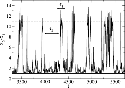
The basic phenomenology of the model is illustrated in Fig. 1. The relative distance, $y=x_{2}-x_{1}$, between particles fluctuates in time showing time intervals of average lifetime $\tau_{2}$, when they are confined to the same well ($y\sim d$) alternated with intervals, of average lifetime $\tau_{1}$, when they sojourn in separate wells ($y\sim L$). Thus, the system behaviour shows the existence of two different time scales $\tau_{1}$ and $\tau_{2}$ employed to characterize two regimes.

Figure 1: Relative distance $x_{2}-x_{1}$ as a function of time for a system with $r=0.9$ and $T_{b}=4.0$. The solid line indicates the diameter of the rods, the dashed marks the well separation $L\simeq 10.95$.

We shall see that, as the driving intensity, $T_{b}$, or inelasticity, $r$, are varied, the system undergoes a crossover from the regime in which particles are far apart most of the time (i.e. $\tau_{1}>\tau_{2}$), to a clusterized regime characterized by $\tau_{1}<\tau_{2}$. Moreover, we shall show that the dependence of $\tau_{2}$ and $\tau_{1}$ on the model parameters can be captured by a simple extension of formula (3), replacing $T_{b}$ by the two different kinetic temperatures

$$T_{2} = \lim_{t\to\infty}\frac{1}{2t_{2}}\int_{0}^{t}ds\bigg{(}v^{2}_{1}(s)+v^{2}_{2}(s)\bigg{)}\Theta[x_{1}(s)x_{2}(s)]$$ (4)

$$T_{1} = \lim_{t\to\infty}\frac{1}{2t_{1}}\int_{0}^{t}ds\bigg{(}v^{2}_{1}(s)+v^{2}_{2}(s)\bigg{)}\Theta[-x_{1}(s)x_{2}(s)]$$ (5)

where $t_{1}$ and $t_{2}$ are the times the particles spend, during $[0,t]$, in different wells or in the same one respectively. The temperature $T_{2}$ represents the velocity variance conditioned to the fact that the two particles belong to the same well, whereas $T_{1}$ is the same quantity when these move in different wells.

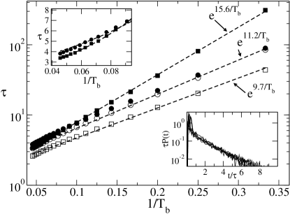
Two physical effects are present: the hard core repulsion and the inelasticity of collisions. For the sake of clarity, let us begin the dicussion with the elastic system ($r=1$). In this case, we deal with an equilibrium system - the measured $T_{2}$ and $T_{1}$ coincide with the heat bath temperature $T_{b}$ distribuz - and therefore, we expect that the most probable configuration minimizes the free energy. This configuration is constituted by a single particle in each well, and corresponds to the condition $\tau_{1}>\tau_{2}$. The results of simulations, shown in Fig. 2, verify this scenario. How do we quantify these escape times? As displayed in Fig. 2, $\tau_{2}$ and $\tau_{1}$ still follow the Arrhenius exponential behavior of Eq. (3), however, with a suitable paremeter renormalization:

$$\tau_{k}\approx\exp\big{[}\frac{W_{k}}{T_{k}}\big{]},$$ (6)

where $k=(1,2)$ indicates single or double occupation, $W_{1}=\Delta U$ and $W_{2}=\Delta U-\delta U<\Delta U$. The correction $\delta U$ takes into account the effect of the excluded volume repulsion: when two grains belong to the same well their center of mass lies higher than if they were in separate wells. This determines a reduction $\delta U=a(d/2)^{2}+b/4(d/2)^{4}$ of the effective energy barrier and makes $\tau_{2}<\tau_{1}$. This is a typical correlation effect, because the repulsion renders less likely, with respect to the non interacting case, the double occupancy of a well. The smaller the ratio between the well width and the particle diameter, the stronger the reduction of the escape time Tarazona .

Figure 2: Arrhenius plot of mean escape times $\tau$. Open symbols refer to elastic case: the escape time is $\tau_{1}$ (circles) when a well is singly occupied, $\tau_{2}$ (squares) when a well is doubly occupied. Full symbols, instead, correspond to the inelastic system ($r=0.9$). Linear behaviour indicates the validity of Kramers theory with renormalized parameters and the slopes agree with values obtained from Eq. (6). Upper inset: enlargement of the crossover region. Lower inset: Data collapse of distribution of escape times for different temperatures. The arguments of the exponentials (dashed lines) in the same figure have been obtained by applying formula (6). The overall agreement between the above prediction and the values of $\tau_{1}$ and $\tau_{2}$ obtained by simulation is rather good.

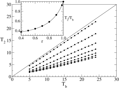
The above scenario changes in the presence of inelasticity ($r<1$) because dissipation tends to promote the double occupation of a well. Thus, upon lowering the temperature $T_{b}$, we expect a crossover from the regime, where the double occupancy of a well is unfavoured (i.e. $\tau_{2}<\tau_{1}$), to the regime, where particles spend most of the time together in the same well i.e. $\tau_{2}>\tau_{1}$. In Fig. 2, for inelasticity $r=0.9$, this crossover is observed and occurs at $T_{b}\simeq 10.0$ (upper inset). This behavior is the analogue of that reported by several authors Eggers ; Brey . The origin of the crossover lies on the fact that, in the inelastic system, temperatures $T_{2}$ and $T_{1}$ are no more equal to $T_{b}$ and furthermore $T_{2}<T_{1}$. Thus, the mean lifetime of the clusterized and non clusterized regimes can be still described by expressions (6), but now the temperature difference competes with the excluded volume correction, eventually leading to $\tau_{2}>\tau_{1}$. A simple argument can be used to estimate the shift of $T_{2}$ from $T_{b}$. For moderate driving intensity, $T_{1}$ is nearly equal to $T_{b}$, while $T_{2}$ is lower than $T_{b}$ by a factor which depends on the inelasticity. In Fig. 3 we show these temperatures as functions of $T_{b}$. It can be observed in Fig.  3 that $T_{2}$ varies linearly with $T_{b}$ and its slope is a decreasing function of the inelasticity $(1-r)$. A good estimate of temperature $T_{2}$ can be obtained by considering the two particles in a single harmonic well $V(x)=\omega^{2}_{min}x^{2}/2$. Balancing the power dissipated by collisions $-(1-r^{2})\nu\overline{(v_{2}-v_{1})^{2}}/4$ and viscous damping ($-2\gamma T_{2}$) with the power supplied by the external source ($2\gamma T_{b}$) we arrive to the expression:

$$T_{2}=\frac{T_{b}}{1+\frac{\nu}{4\gamma}(1-r^{2})}$$ (7)

where the collision frequency $\nu$ is estimated as $\omega_{min}/\pi$ (the factor $2$ stems from the excluded volume effect). We have assumed that the precollisional relative velocity $\overline{(v_{2}-v_{1})^{2}}\simeq(<v_{1}^{2}>+<v_{2}^{2}>)=2T_{2}$. An improved value of $T_{2}$ results when using the value of $\nu$ obtained from the simulation. The dependence of the formula on the restitution coefficient is shown in the inset of Fig. 3.

In the lower inset of Fig. 2 we plot the probability distributions of escape times $\tau_{1}$ and $\tau_{2}$ for several simulations. All the distributions are characterized by a peak at the origin and an exponential tail. When rescaled to have the same average, all the tails collapse to a single curve. Such exponential tails are typical of the original Kramers model for thermally activated barrier crossing.

Figure 3: Plot of the temperature $T_{2}$ vs. $T_{b}$ for various choices of the elasticity parameter $r$. From top to bottom the curves indicate $r=0.98,0.9,0.8,0.7,0.6,0.5,0.4$. As $r$ grows toward the value $1$ the lines approach the diagonal (solid line) where $T_{2}=T_{b}$. The inset shows the ratio $T_{2}/T_{b}$ obtained by the slopes of $T_{2}$ vs. $T_{b}$ for the same values of $r$. The continuous line indicates the theoretical estimate given by formula (7).

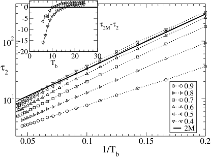
A new non trivial phenomenon occurs at low temperature and small restitution coefficient. The escapes from a doubly occupied well become correlated, i.e. the transition takes place as a collective motion of the two particles. In other words, when the inelasticity is strong the relative motion of the two particles, due to repeated collisions, becomes frozen and they tend to form a “molecule”. It is easy to show (within an harmonic treatment of the potential) that the noise acting on the center of mass coordinate corresponds to a reduced heat bath temperature $T_{b}/2$. We computed the exit time $\tau_{m}$ for the “molecule” and compared it with the characteristic times $\tau_{2}$ for several values of the inelasticity. As shown in Fig. 4, when the driving temperature decreases, $\tau_{2}$ corresponding to a strongly inelastic system ($r=0.5$) exceeds $\tau_{m}$. This is the signature that the most probable evolution of a doubly occupied state involves the simultaneous hopping of the two particles in the adjacent well, without breaking the pair. This freezing of the internal motion, is related to the problem of the dynamics of two randomly accelerated particles on a line considerd in Refs. Bray ; Burkhardt , or equivalently, to the problem of a single particle moving on the half line ($x>0$) in the presence of an inelastic (impenetrable) wall. The authors predicted that at fixed driving intensity and for $r$ below a critical value, $r=r_{c}$, the particle localises at the wall. We argue that the localization mechanism is identical to that leading to the formation of the “molecule” in our model.

Figure 4: Arrhenius plot of the mean escape times $\tau_{2}$ versus $1/T_{b}$ for several values of $r$. Thick solid line indicates the escape time $\tau_{m}$ of single particle of mass $2M$ corresponding to simultaneous jumps. At about $T_{b}=10$ and $r=0.5$ we observe a crossover between $\tau_{2}$ and $\tau_{m}$ signalling the formation of a stable molecule. The inset shows the difference $\tau_{m}-\tau_{2}$ vs. $T_{b}$ to pinpoint the crossover where $\tau_{m}\simeq\tau_{2}$

In summary, whereas previous studies on compartimentalized systems were based on coarse grained descriptions of granular gases, our approach focuses on the statistical description of particle motions by means of a characterization of their stochastic fluctuations. The basic phenomenology illustrated above, suggests that after a suitable redefinition of parameters ($T_{b}$ replaced by $T_{2}$ and $\Delta U$ by $W_{2}$) the present problem can be mapped onto that of a single particle hopping between two wells at different temperatures $T_{1}$ and $T_{2}$. We have shown how $T_{2}$ decreases with the inelasticity. The local granular temperature is the relevant control parameter in determining the direction of the energy flux (particles flow from hot places to cold places). The activation rates, $\tau_{2}^{-1}$ and $\tau_{1}^{-1}$ display an Arrhenius dependence on the temperatures $T_{1}$ and $T_{2}$, respectively. However, as $r$ decreases further, a deeper scrutiny reveals a more complex scenario. The model displays a further “transition” at even low temperatures because the two rods form a “bound” pair as a result of extremely frequent collisions. The escape from the wells can occur only “in tandem”.

As a natural extension of the present model, due to the continuous interest on transport properties on rough surfaces, compartimentalized systems and ratchets, one could examine the dynamics of an ensemble of grains in a larger number of wells. This would allow to determine explicitly the variation of the granular temperature and of the transition rates with the occupation number of the wells. The latter are key ingredients in hydrodynamic descriptions.

We are in debt to G. Jug for his suggestions and remarks. We acknowledge the support of the Cofin MIUR “Fisica Statistica di Sistemi Classici e Quantistici”.

References

- (1) Granular Gases, vol. 564 of Lectures Notes in Physics, T. Pöschel and S. Luding editors, Berlin Heidelberg, Springer-Verlag (2001).
- (2) I. Goldhirsch and G. Zanetti, Phys. Rev. Lett. 70 1619 (1993).
- (3) A. Baldassarri, U. Marini Bettolo Marconi and A.Puglisi, Phys. Rev.E, 65, 051301 (2002).
- (4) U. Marini Bettolo Marconi and A.Puglisi Phys. Rev. E 66, 011301 (2002).
- (5) A.Kudrolli and J. Henry Phys. Rev. E 62, R1489 (2000).
- (6) H.M. Jaeger, S.R. Nagel and R.P. Behringer, Rev. Mod. Phys. 68, 1259 (1996) and references therein.
- (7) H.J. Schlichting and V. Nordmeier, Math. Naturwiss. Unterr., 49, 323 (1996) (in German).
- (8) J. Eggers, Phys. Rev. Lett. 83, 5322 (1999).
- (9) J. Javier Brey, F. Moreno, R. García-Rojo, and M. J. Ruiz-Montero, Phys. Rev. E 65, 011305 (2002).
- (10) D. van der Meer, K. van der Weele, and D. Lohse, Phys. Rev. Lett. 88, 174302 (2002).
- (11) H. A. Kramers, Physica (Utrecht) 7, 284 (1940).
- (12) P. Hänngi, P. Talkner, M. Borkovec, Rev. Mod.Phys. 62, 251 (1990).
- (13) The external drive is modeled via a stochastic force. See A. Puglisi, V. Loreto, U. M. B. Marconi, A. Petri, and A. Vulpiani, Phys. Rev. Lett. 81, 3848 (1998); A. Puglisi, V. Loreto, U. M. B. Marconi, and A. Vulpiani, Phys. Rev. E 59, 5582 (1999).
- (14) We checked numerically that the velocity distributions for the elastic system were gaussians of variance .
- (15) U. Marini Bettolo Marconi and P.Tarazona, J.Chem.Phys. 110, 8032 (1999).
- (16) S. J. Cornell, M. R. Swift, and A. J. Bray, Phys. Rev. Lett. 81, 1142 (1998).
- (17) T.W. Burkhardt, Phys. Rev. E 63, 011111 (2001).