CCD photometry and new models of 5 minor planets

Abstract

We present new $R$ filtered CCD observations of 5 faint and moderately faint asteroids carried out between October, 1998 and January, 1999. The achieved accuracy is between 0.01–0.03 mag, depending mainly on the target brightness. The obtained sinodic periods and amplitudes: 683 Lanzia – $4\aas@@fstack{h}6\pm 0\aas@@fstack{h}2$, 0.13 mag; 725 Amanda – $>3\aas@@fstack{h}0$, $\geq$0.40 mag; 852 Wladilena – $4\aas@@fstack{h}62\pm 0\aas@@fstack{h}01$, 0.32 mag (December, 1998) and 0.27 mag (January, 1999); 1627 Ivar – $4\aas@@fstack{h}80\pm 0\aas@@fstack{h}01$, 0.77 mag (December, 1998) and 0.92 mag (January, 1999). The Near Earth Object 1998 PG unambiguously showed doubly-periodic lightcurve, suggesting the possibility of a relatively fast precession (P₁=1$\aas@@fstack{h}$3, P₂=5$\aas@@fstack{h}$3).

Collecting all data from the literature, we determined new models for 3 minor planets. The resulting spin vectors and triaxial ellipsoids have been calculated by an amplitude-method. Sidereal periods and senses of rotation were calculated for two asteroids (683 and 1627) by a modified epoch-method. The results are: 683 – $\lambda_{p}=15/195\pm 25^{\circ}$, $\beta_{p}=52\pm 15^{\circ}$, $a/b=1.15\pm 0.05$, $b/c=1.05\pm 0.05$, P_sid=0$\aas@@fstack{d}$1964156$\pm$0$\aas@@fstack{d}$0000001, retrograde; 852 – $\lambda_{p}=30/210\pm 20^{\circ}$, $\beta_{p}=30\pm 10^{\circ}$, $a/b=2.3\pm 0.3$, $b/c=1.2\pm 0.2$; 1627 – $\lambda_{p}=145/325\pm 8^{\circ}$, $\beta_{p}=34\pm 6^{\circ}$, $a/b=2.0\pm 0.1$, $b/c=1.09\pm 0.05$, P_sid=0$\aas@@fstack{d}$1999154$\pm$0$\aas@@fstack{d}$0000003, retrograde. The obtained shape of 1627 is in good agreement with radar images by Ostro et al. (1990).

1 Introduction

Ground-based modelling of the shape and the rotation of the minor planets requires high precision and long-term photometric observations. With the advent of the CCD era it has become possible to study much fainter minor planets than previously. The photometric methods of modelling are based on multi-opposition lightcurves of full phase coverage obtained at very different longitudes (De Angelis 1993, Detal et al. 1994, Szabó et al. 1999). Another important aspect is to detect possible collisional effects, e.g. multiperiodic lightcurves due to binarity or precession, as they may yield insights into the recent solar system evolution.

We started a long-term observational project addressed to photometric monitoring of selected minor planets. The observing programme consists of asteroids with available multi-opposition lightcurves enabling application of different photometric methods in order to model their shape and rotation. First results of this project have already been published in Sárneczky et al. (1999) and Szabó et al. (1999). The main aim of this paper is to present new CCD observations carried out between October, 1998 and January, 1999 and models for 3 minor planets. Observations, their limitations and applied methods are discussed in Sect. 2, while Sect. 3 deals with the detailed observational results.

2 Observations and modelling methods

We carried out $R_{C}$ filtered CCD observations at Piszkéstető Station of Konkoly Observatory on ten nights from October, 1998 to January, 1999. The data were obtained using the 60/90/180 cm Schmidt-telescope equipped with a Photometrics AT200 CCD camera (1536x1024 KAF 1600 MCII coated CCD chip). The projected sky area is 29’x18’ which corresponds to an angular resolution of 1$\aas@@fstack{\prime\prime}$1/pixel.

The exposure times were limited by two factors: firstly, the asteroids were not allowed to move more than the FWHM of the stellar profiles (varying from night to night) and secondly, the signal-to-noise (SN) ratio had to be at least 10. This latter parameter was estimated by comparing the peak pixel values with the sky background during the observations. The journal of observations is summarized in Table 1.

Table 1: The journal of observations. ($r$ – geocentric distance; $\Delta$ – heliocentric distance; $\lambda$ – ecliptic longitude; $\beta$ – ecliptic latitude; $\alpha$ – solar phase angle; aspect data are referred to 2000.0)

Date	RA	Decl.	$r$(AU)	$\Delta$(AU)	$\lambda$	$\beta$	$\alpha$
683 Lanzia
1998 12 14/15	00 12.78	+19 58.9	3.25	2.82	20	18	17
1998 12 16/17	00 13.78	+19 49.5	3.25	2.84	20	18	17
725 Amanda
1999 01 26/27	06 31.61	+27 13.5	2.34	1.44	110	24	12
852 Wladilena
1998 12 12/13	11 40.37	+27 28.2	2.98	2.71	163	23	19
1998 12 14/15	11 41.67	+27 31.9	2.98	2.68	163	23	19
1998 12 16/17	11 42.89	+27 36.2	2.98	2.65	163	23	19
1999 01 24/25	11 47.52	+30 52.9	2.95	2.18	170	19	14
1627 Ivar
1998 12 14/15	05 03.41	+10 30.4	2.22	1.26	76	$-$12	6
1998 12 15/16	05 02.00	+10 32.6	2.23	1.26	76	$-$12	6
1998 12 16/17	05 00.62	+10 34.9	2.23	1.27	76	$-$12	7
1999 01 22/23	04 30.95	+13 09.2	2.35	1.65	85	$-$13	20
1998 PG
1998 10 23/24	23 47.69	+09 15.0	1.23	0.26	2	9	25
1998 10 26/27	23 55.11	+08 26.9	1.23	0.27	2	7	25
1998 10 27/28	23 57.63	+08 11.6	1.23	0.27	2	7	26

The image reduction was done with standard IRAF routines. The relatively high electronic noises and low angular resolution did not permit the use of psf-photometry and that is why a simple aperture photometry was performed with the IRAF task noao.digiphot.apphot.qphot. Unfortunately other filters were not available during the observing run and consequently we could obtain only instrumental differential $R$ magnitudes in respect to closely separated comparison stars. The precision was estimated with the rms scatter of the comp.$-$check magnitudes (tipically 0.01–0.03 mag).

We have also investigated the possible colour effects in neglecting standard photometric transformations. We made an $R$ filtered 60-seconds CCD image of open cluster M67 on December 14, 1998. This cluster contains a widely used sequence of photometric standard stars (Schild 1983). We determined the instrumental magnitude differences in respect to star No. 81 in Schild (1983), which various colour indices are close to zero ($(B-V)=-0.098$, $(V-R)_{C}=-0.047$ mag). The studied standards were stars No. 106, 108, 117, 124, 127, 128, 129, 130, 134 and 135, following Schild’s notation. We plotted the resulting differences ($\Delta R_{ins}-\Delta R_{std}$) vs. $(B-V)$ and $(V-R)_{C}$ in Fig. 1. For a wide colour range they do not differ more than 0.1 mag, while the colour dependence is quite weak. Therefore, the obtained instrumental $R$-amplitudes of minor planet lightcurves are very close to the standard ones, allowing reliable comparison with other measurements.

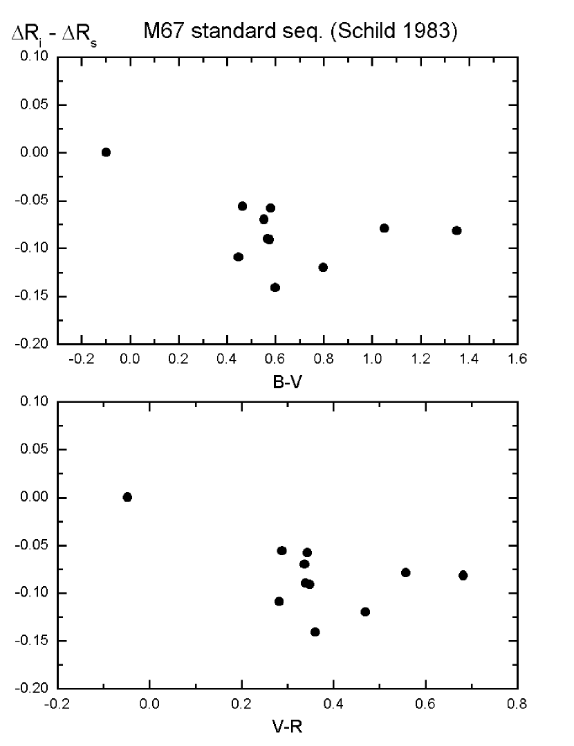
Figure 1: The colour dependence of instrumental minus standard magnitude differences for selected photometric standard stars in M67.

The presented magnitudes throughout the paper are based on magnitudes of the comparison stars taken from the Guide Star Catalogue (GSC) (Table 2). Therefore, their absolute values are fairly uncertain (at level of $\pm$0.2–0.3 mag). Fortunately it does not affect the other photometric parameters needed in the minor planet studies, such as the amplitude, time of extrema, or photometric period. The final step in the data reduction was the correction for the light time. Composite diagrams were calculated using APC11 by Jokiel (1990) and are also light time corrected. Times of zero phase are included in the individual remarks.

Table 2: The comparison stars. The typical uncertainty in the magnitude values is as large as $\pm$0.2-0.3 mag.

Date	Comp.	$m$(GSC)
683 Lanzia
1998 12 14	GSC 1182 337	15.3
1998 12 16	GSC 1182 85	14.4
725 Amanda
1999 01 26	GSC 1887 1325	12.3
852 Wladilena
1998 12 12	GSC 1984 2286	12.7
1998 12 14	GSC 1984 2516	12.0
1998 12 16	GSC 1984 2496	13.8
1999 01 24	GSC 2524 1778	12.6
1627 Ivar
1998 12 12	GSC 702 759	12.6
1998 12 14	GSC 689 1331	12.8
1998 12 16	GSC 689 2101	12.6
1999 01 22	GSC 681 519	13.7
1998 PG
1998 10 23	GSC 1170 1119	14.2
1998 10 24	GSC 1171 632	14.3
1998 10 26	GSC 1171 1424	14.5

Two methods were applied for modelling. The first is the well-known amplitude-method described, e.g., by Magnusson (1989) and Michałowski (1993). For this the amplitude information is used to determine the spin vector and the shape. An important point is that the observed $A(\alpha)$ amplitudes at solar phase $\alpha$ should be reduced to zero phase ($A(0^{\circ})$), if possible, by a simple linear transformation in form of $A(\alpha)=A(0^{\circ})(1+m\alpha)$. $m$ is a parameter, which has to be determined individually and that can be difficult, or even impossible if there are insufficient observations (Zappala et al. 1990).

The other possibility is to examine the times of light extrema (“epoch-methods”, “E-methods”). In this paper a modified version was used, which gives the sense of the rotation unambiguously. The pole coordinates can be also estimated independently. Further details can be found in Szabó et al. (1999) and Szabó et al. (in prep.), here we give only a brief description.

The initial idea is that the prograde and retrograde rotation can be distinguished by following the virtual shifts of moments of light extrema (e.g. times of minima). From a geocentric point of view, a full revolution around the Earth causes one extra rotational cycle to be added (retrograde rotation) or subtracted (prograde rotation) to the observed number of rotational cycles during that period. The virtual shifts increase or decrease monotonically and their cumulative change is exactly one period over one revolution. Therefore, plotting the observed minus calculated (O$-$C) times of minima versus the geocentric longitude, we get a monotone function ascending or descending by the value of the period. The definition of the observed O$-$C is as follows:

$$O-C=T_{\rm min}-(E_{\rm 0}+N\cdot P_{\rm sid})\equiv\langle{\Delta T\over P_{\rm sid}}\rangle P_{\rm sid}$$ (1)

where $T_{\rm min}$ means the observed time of minimum, $E_{\rm 0}$ is the epoch, while the $N$ integer number denotes the cycles (e.g. the number of rotation) of $P_{\rm sid}$ period between the observed extremum and the epoch. ${\Delta T}$ means the time interval between $T_{\rm min}$ and $E_{\rm 0}$, and $\langle\rangle$ denotes fractional part. The theoretical O$-$C curve depends on the pole coordinates:

$$O-C^{\prime}:={O-C\over P_{\rm sid}}={1\over\pi}{\rm arctan}{{\rm tan}(\Lambda-\lambda_{p})\over{\rm sin}(\beta_{p}-B)}$$ (2)

where $\Lambda$ and $B$ denote geocentric longitude and latitude; ${\lambda{\rm p}}$ and ${\beta{\rm p}}$ are the pole coordinates.

The main difference between the classical E-methods and this O$-$C’ method is that time dependence is transformed into the geocentric longitude domain. Because of the system’s basic symmetries, the O$-$C’ diagrams are calculated for a half revolution and with the half sidereal period. The fitting procedure consists of altering $P_{sid}$ until the observed times of minima do not give a monotone O$-$C’ diagram showing an increase or decrease of exactly 1. Fitting a theoretical curve (Eq. 2) to the observed points, the pole coordinates can be also estimated.

3 Discussion

683 Lanzia

This minor planet was discovered by M. Wolf in Heidelberg, on July 23, 1909. It was observed in the 1979, 1982, 1983-1984, 1987 oppositions (Carlsson & Lagerkvist 1981, Weidenschilling et al. 1990). Carlsson & Lagerkvist (1981) determined a rotation period of 4$\aas@@fstack{h}$322 and an amplitude of 0.14 mag. On the other hand, Weidenschilling et al. (1990) measured a period of 4$\aas@@fstack{h}$37 with an amplitude of 0.12 mag.

Our observations in 1998 suggest a period of 4$\aas@@fstack{h}$6$\pm$0$\aas@@fstack{h}$2 with an amplitude of 0.13$\pm$0.01. Composite diagrams calculated with previously published periods between 4$\aas@@fstack{h}$3-4$\aas@@fstack{h}$4 have much larger scatter. The light-time corrected composite diagram is presented in Fig. 2. The zero phase is JD 2451162.3169.

Based on earlier data (see Table 3), a new model has been determined with amplitude method. The observed amplitudes vs. ecliptic longitudes with the fit are plotted in Fig. 3. The resulting triaxial ellipsoid has the following parameters: a/b=1.15$\pm$0.07, b/c=1.05$\pm$0.05, while the spin vector’s coordinates are $\lambda_{p}=15/195\pm 25^{\circ}$, $\beta_{p}=52\pm 15^{\circ}$, respectively. We could not reduce the observed amplitudes to zero solar phase, since the actual value of $m$ parameter (e.g. Zappala et al. 1990) could not be estimated by the data sequence or asteroid classification. Also we have to note that a mixture of $V$ and $R$ amplitudes was used, thus the model should be considered as an approximate one. The O$-$C’ model has also been determined (Fig. 4). For reducing the errors, lightcurves obtained between October, 1983 and February, 1984, were composed and one time of minimum was determined from this composite lightcurve. The resulting sidereal period is $P_{sid}$=0$\aas@@fstack{d}$1964156$\pm$0$\aas@@fstack{d}$0000001 with retrograde rotation.

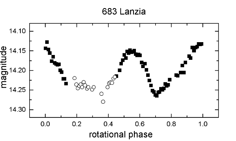
Figure 2: The composite $R$ lightcurve of 683 (symbols: solid squares – December 14; open circles – December 16).

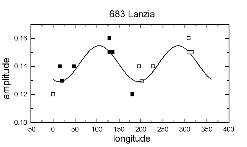
Figure 3: The observed amplitudes vs. longitudes with the determined fit for 683 Lanzia

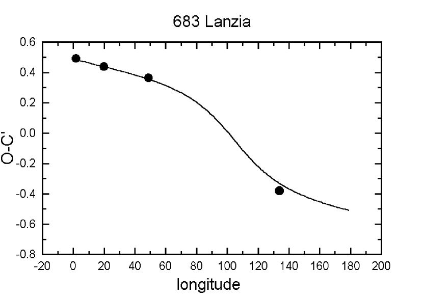
Figure 4: The observed O$-$C’ values fitted with the model for 683 Lanzia

Table 3: Published photometries of 683 Lanzia

Date	$\lambda$	$\beta$	$\alpha$	A	tmin	ref.
1979 03 19,20	182	$-$27	9	0$\aas@@fstack{m}$12	43963.452	(1)
1982 12 16	49	9	11	0.14	45319.591	(2)
1983 10 12,13	130	$-$9	18	0.15	45650.871	(2)
1983 11 15	137	$-$13	19	0.15	45650.871	(2)
1984 02 21	129	$-$23	10	0.16	45650.871	(2)
1987 10 19	16	23	7	0.12	47118.538	(2)
1998 12 14,16	20	18	17	0.13	51162.275	p.p.

References: (1) – Carlsson & Lagerkvist 1981; (2) – Weidenschilling et al. 1990

725 Amanda

It was discovered by J. Palisa in Vienna, on October 21, 1911. To our knowledge, the only one photometry of 725 in the literature is that of Di Martino et al. (1994) carried out in 1985. They determined a sinodic period of 3$\aas@@fstack{h}$749 associated with a full variation of 0.3 mag. Our observations do not exclude that period, as they suggest a possible value around 4 hours. Unfortunately the data cover only 3 hours, thus we could not draw a firm conclusion. The observations were made under fairly unfavourable conditions, which is illustrated with the comp–check curve bearing a relatively high scatter (about $\pm$0.03 mag). It is presented together with the observed lightcurve in Fig. 5.

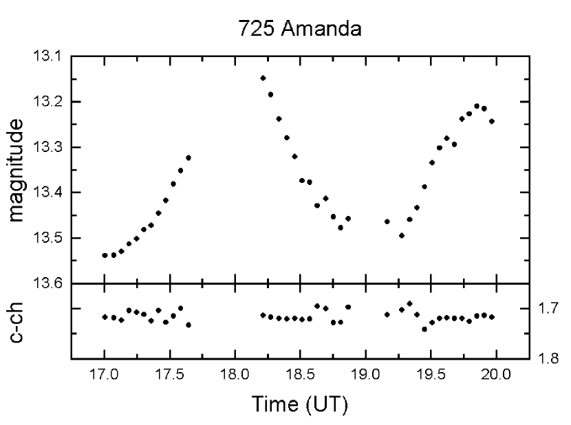
Figure 5: The R lightcurve of 725 on January 26, 1999.

852 Wladilena

This asteroid was discovered by S. Belyavskij in Simeis, on April 2, 1916. Its earlier photometric observations were carried out in 1977, 1982 and 1993 (Tedesco 1979, Di Martino & Cacciatori 1984, De Angelis & Mottola 1995). The observed light variation in 1998 had an amplitude of 0.32 mag, while the period was 4$\aas@@fstack{h}$62$\pm$0$\aas@@fstack{h}$01. This is in very good agreement with results by De Angelis & Mottola (1995), who found a period value of 4$\aas@@fstack{h}$613. The light time corrected composite diagram is presented in Fig. 6. The zero phase is at 2451160.5904. The lightcurve has remarkable asymmetries – the brighter maximum is rather sharp, its hump is exactly two times shorter than the other one. There are also small amplitude, short-period humps on the longer descending branch. These phenomena can be more or less identified in the previous measurements too. That is why we carried out a second observing run on January 24, 1999. We wanted to check the reality of these irregularities. The lightcurve revealed the same asymmetries as those of observed one month earlier (Fig. 7). This may refer to a shape with sharp asymmetries, e.g. something similar to a jagged tenpin.

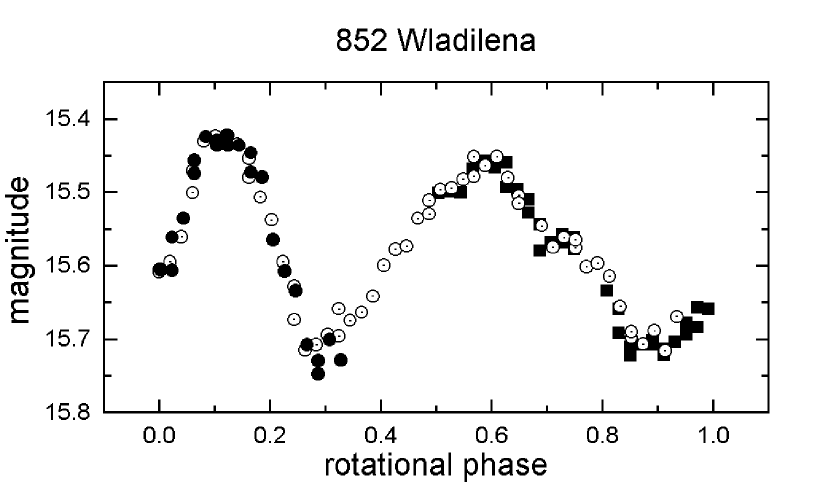
Figure 6: The composite R lightcurve of 852 (symbols: solid circles – December 12; dotted circles – December 14; solid squares – December 16).

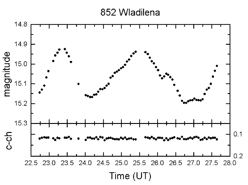
Figure 7: The R lightcurve of 852 on January 24, 1999

We have tried to determine a new model using the earlier data summarized in Table 4. Unfortunately, the measurements have such a distribution along the longitude that reliable modelling is difficult. This is shown in Fig. 8, where the observed amplitudes vs. ecliptic longitudes are plotted with an approximate fit. The resulting parameters are as follows: a/b=2.3$\pm$0.3, b/c=1.2$\pm$0.2, $\lambda_{p}=30/210\pm 20^{\circ}$, $\beta_{p}=30\pm 10^{\circ}$. The pole coordinates are in considerable agreement with those of by De Angelis & Mottola (1995), who determined two possible solutions: (1) $\lambda_{p}=53\pm 6^{\circ}$, $\beta_{p}=24\pm 20^{\circ}$ and (2) $\lambda_{p}=235\pm 6^{\circ}$, $\beta_{p}=21\pm 20^{\circ}$.

Table 4: Published photometries of 852 Wladilena

Date	$\lambda$	$\beta$	$\alpha$	A	ref.
1977 02 14	139	31	10	1$\aas@@fstack{m}$12	(1)
1982 10 18	6	$-$10	10	0.37	(2)
1993 11 8,10	33	$-$8	3	0.23	(3)
1998 12 12-16	163	23	19	0.32	p.p.
1999 01 24	170	19	14	0.27	p.p.

References: (1) – Tedesco 1979; (2) – Di Martino & Cacciatori 1984; (3) De Angelis & Mottola 1995

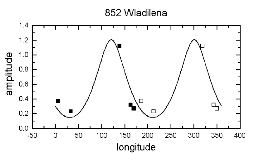
Figure 8: The observed amplitudes vs. longitudes with the determined fit for 852 Wladilena

1627 Ivar

This Earth-approaching asteroid was discovered by E. Hertzsprung in Johannesburg, on September 25, 1929. There are four photometric observations in the literature (Hahn et al. 1989, Velichko et al. 1990, Hoffmann & Geyer 1990, Chernova et al. 1995) and one radar measurement by Ostro et al. (1990). The previously determined periods scatter around 4$\aas@@fstack{h}$8, thus our resulting 4$\aas@@fstack{h}$80$\pm$0.01 is in perfect agreement with earlier results. The amplitude changed significantly over a period of one month, as it was 0.77 mag and 0.92 mag in December, 1998 and January, 1999, respectively. The composite lightcurve is presented in Fig. 9, while the single lightcurve obtained in January is plotted in Fig. 10.

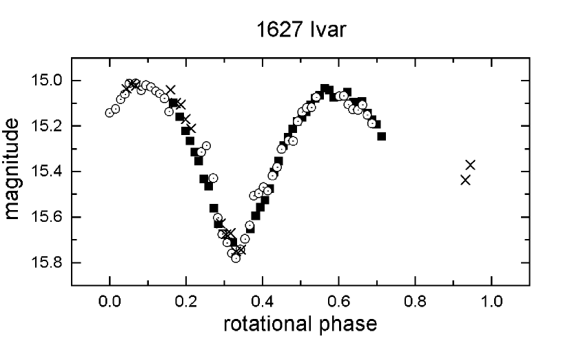
Figure 9: The composite $R$ lightcurve of 1627 (symbols: solid squares – December 14; dotted circles – December 15; crosses – December 16).

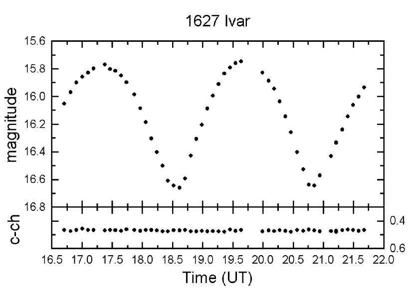
Figure 10: The $R$ lightcurve of 1627 on January 22, 1999

Table 5: Published photometries of 1627 Ivar

Date	$\lambda$	$\beta$	$\alpha$	A	tmin	ref.
1985 06 13	317	29	48	0$\aas@@fstack{m}$35	46226.750	(1)
1985 08 31	15	$-$21	32	0.55	46258.703	(1)
1985 10 16	4	$-$23	20	0.63	46287.184	(1)
1989 05 01-23	203	25	20	1.0	47647.402	(2)
1989 06 15-23	201	21	51	1.12	47647.402	(2)
1989 07 14-19	213	14	60	1.45	47721.565	(2)
1990 05 11-14	204	25	24	1.08	48029.439	(3,4)
1998 12 14,16	76	$-$12	79	0.77	51162.295	p.p.
1999 01 26	87	$-$13	18	0.92	51201.171	p.p.

References: (1) – Hahn et al. 1989; (2) – Chernova et al. 1995; (3) – Velichko et al. 1990; (4) Hoffmann & Geyer 1990

A new amplitude model has been determined after collecting all available data (Table 5). The observed amplitudes were reduced to zero solar phase. First of all, the $m$ parameter was derived from our measurements. The observed amplitudes in December, 1998 and in January, 1998 were compared. As the longitudes differ by only 10^∘, and the difference between the corresponding phases is quite high (13^∘), the amplitude change can be mostly associated with the phase change. The result is $m=0.018$. We have also corrected other amplitudes to zero solar phase and fitted the amplitude variations along the longitude. The corresponding parameters are: a/b=2.0$\pm$0.1, b/c=1.09$\pm$0.05, $\lambda_{p}=145/325\pm 8^{\circ}$, $\beta_{p}=34\pm 6^{\circ}$. The reduced amplitudes with the determined fit is presented in Fig. 11. The reliability of this model was tested by a direct comparison with radar images of Ostro et al. (1990). This is shown in Fig. 12, where we used Fig. 5 taken from Ostro et al. (1990) with kind permission of the first author. The similarity is evident.

The O$-$C’ method was used to determine the sidereal period and the sense of the rotation. The results are P_sid=0$\aas@@fstack{d}$1999154$\pm$0$\aas@@fstack{d}$0000003, retrograde rotation with $\lambda_{p}=143\pm 8^{\circ}$, $\beta_{p}=-37\pm 6^{\circ}$ pole coordinates. The agreement between the poles obtained by different methods is very good. The sidereal period agrees well with results of Lupishko et al. (1986) – 0$\aas@@fstack{d}$19991, prograde –, but the senses are in contradiction. The fitted O$-$C’ diagram is presented in Fig. 13.

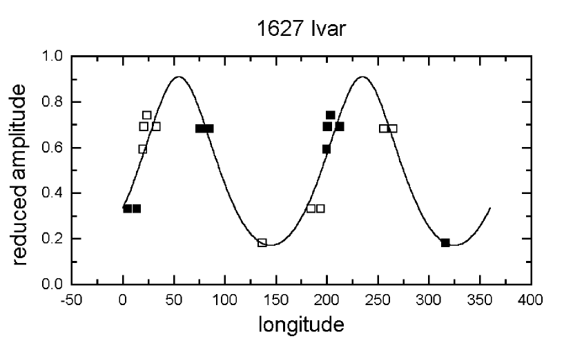
Figure 11: The reduced amplitudes vs. longitudes with the determined fit for 1627 Ivar

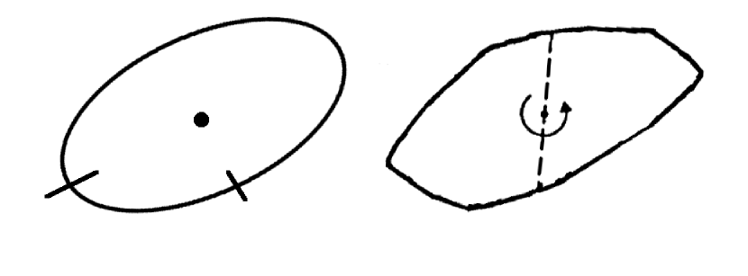
Figure 12: A pole-on view of the photometric model (left) and radar profile (right) of 1627 Ivar. The small ticks correspond to the uncertainties of the fit.

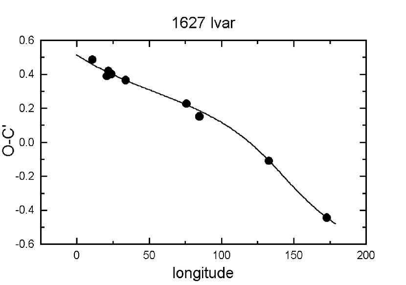
Figure 13: The observed O$-$C’ values fitted with the model for 1627 Ivar

1998 PG

The Near Earth Object (NEO) 1998 PG was discovered by the LONEOS project in Flagstaff, on August 3, 1998. We observed about 80 days after the discovery, in October, 1998. We found complex, strongly scattering lightcurves (two of them are shown in Figs. 14–15), which did not show any usual regularity. Therefore, we performed a conventional frequency analysis by calculating Discrete Fourier Transform (DFT) of the whole dataset (Fig. 16). Data obtained on October 27 are too noisy, thus we excluded them from the period determination.

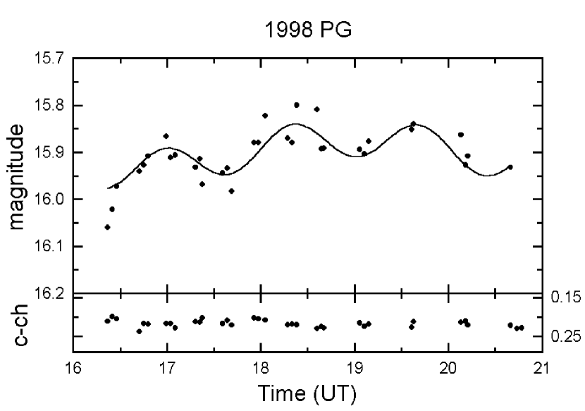
Figure 14: The observed and fitted $R$ lightcurves of 1998 PG on October 23, 1998

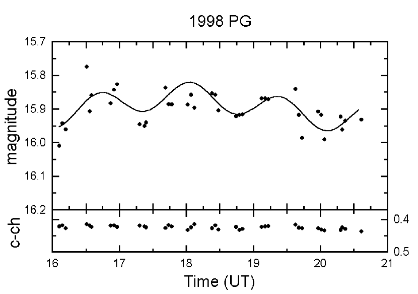
Figure 15: The same as in Fig. 14 on October 26, 1998

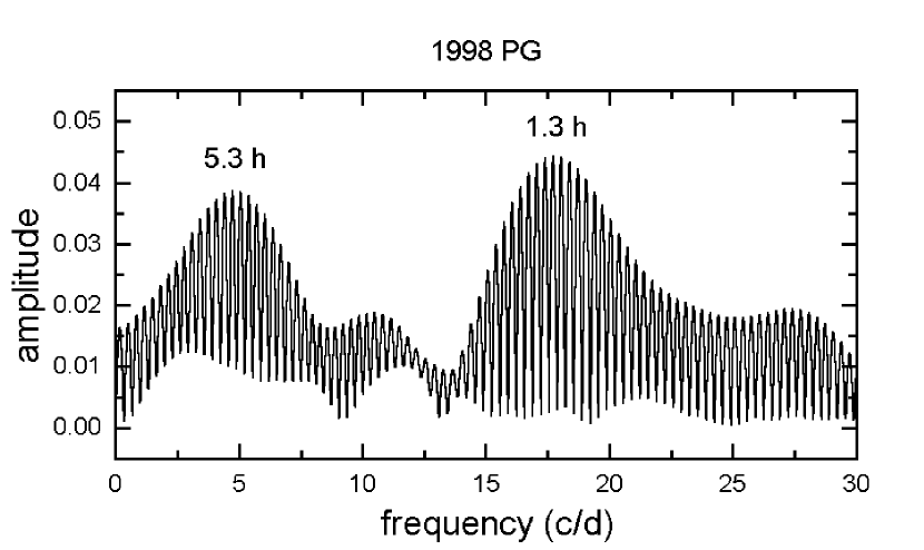
Figure 16: Fourier spectrum of 1998 PG.

The determined periods are 1$\aas@@fstack{h}$3 and 5$\aas@@fstack{h}$3, although these values have large uncertainties (about 10–15%). Assuming that the shorter period is due to rotation, we get a rotational period of 2$\aas@@fstack{h}$6. We note that our period values do not contradict those obtained by P. Pravec and his collaborators, who found $P_{rot}$=2$\aas@@fstack{h}$517 and $P_{2}\approx$ 7$\aas@@fstack{h}$0 (Pravec 1998, personal communication). The reason for doubly periodic lighcurve can be precession and/or binarity. The observed rate of multiperiodic lightcurves among NEOs is quite high (see, e.g., Pravec 1999), but the underlying physical processes can only be identified with more detailed observations than we have on 1998 PG. Therefore, we conclude that we may have found evidence for precession in 1998 PG, but other explanations cannot be excluded.

We summarize the resulting sinodic periods, amplitudes and models in Table 6.

Table 6: The determined periods, amplitudes, spin vectors and shapes.

Asteroid	P${}_{sin}(h)$	P${}_{sid}(d)$	A (mag)	$\lambda_{p}$	$\beta_{p}$	a/b	b/c	method
683	4.6		0.13	15/195$\pm$25	52$\pm$15	1.15$\pm$0.05	1.05$\pm$0.05	A
		0$\aas@@fstack{d}$1964156 R						O$-$C
725	$\geq$3		$\geq$0.4	–	–	–	–	A
852	4.62		0.32, 0.27	30/210$\pm$20	30$\pm$10	2.3$\pm$0.3	1.2$\pm$0.2	A
1627	4.80		0.77, 0.92	145/325$\pm$8	34$\pm$6	2.0$\pm$0.1	1.09$\pm$0.05	A
		0$\aas@@fstack{d}$1999154 R		143	$-$37			O$-$C
1998 PG	2.6		0.09					Fourier
—	5.3		0.08					Fourier

- (1) Carlsson M., Lagerkvist C.I., 1981, A&AS 45, 1
- (2) Chernova G.P., Kiselev N.N., Krugley Yu.N. et al., 1995, AJ 110, 1875
- (3) De Angelis G., 1993, P&SS 41, 285
- (4) De Angelis G., Mottola S., 1995, P&SS 43, 1013
- (5) Detal A., Hainaut O., Pospieszalska-Surdej A. et al., 1994, A&A 281, 269
- (6) Di Martini M., Cacciatori S., 1984, Icarus 60, 75
- (7) Di Martino M., Dotto E., Barucci M.A. et al., 1994, Icarus 109, 210
- (8) Hahn G., Magnusson P., Harris A.W. et al., 1989, Icarus 78, 363
- (9) Hoffmann M., Geyer E.H., 1990, AcA 40, 389
- (10) Jokiel R., 1990, Astronomical Observatory of Adam Mickiewicz University, Poznan
- (11) Lupishko D.F., Velichko F.P., Shevchenko V.G., 1986, KFNT, 2, 5, 39
- (12) Magnusson P., 1989, in: Asteroids II, University of Arizona Press, p.1180
- (13) Michałowski T., 1993, Icarus 106, 563
- (14) Ostro S. J., Campbell D. B., Hine A. A. et al., 1990, AJ 99, 2012
- (15) Pravec P., 1999, http://sunkl.asu.cas.cz/~ppravec/
- (16) Sárneczky K., Szabó Gy., Kiss L.L., 1999, A&AS 137, 363
- (17) Szabó Gy., Sárneczky K., Kiss L.L., 1999a, Contrib. Skalnate Pleso Obs. 28, in press
- (18) Schild R.E., 1983, PASP 95, 1021
- (19) Tedesco E.F., 1979, Ph.D. dissertation, New Mexico State University
- (20) Velichko F.P., Krugly Y.N., Lupishko D.F., Mohamed R.A., 1990, Astron. Tsirk. No.1546, 39
- (21) Weidenschilling S.J., Chapman C.R., Davis D.R. et al., 1990, Icarus 86, 402
- (22) Zappala V., Cellino A., Barucci A.M. et al., 1990, A&A 231, 548