Multiperiodicity in semiregular variables
Abstract
We present a detailed period analysis for 93 red semiregular variables by means of Fourier and wavelet analyses of long-term visual observations carried out by amateur astronomers. The results of this analysis yield insights into the mode structure of semiregular variables and help to clarify the relationship between them and Mira variables.
After collecting all available data from various international databases (AFOEV, VSOLJ, HAA/VSS and AAVSO) we test the accuracy and reliability of data. We compare the averaged and noise-filtered visual light curves with simultaneous photoelectric V-measurements, the effect of the length versus the relatively low signal-to-noise ratio is illustrated by period analysis of artificial data, while binning effects are tested by comparing results of frequency analyses of the unbinned and averaged light curves.
The overwhelming majority of the stars studied show multiperiodic behaviour. We found two significant periods in 44 variables, while there are definite signs of three periods in 12 stars. 29 stars turned out to be monoperiodic with small instabilities in the period. Since this study deals with the general trends, we wanted to find only the most dominant periods.
The distribution of periods and period ratios is examined through the use of the and plots. Three significant and two less obvious sequences are present which could be explained as the direct consequence of different pulsational modes. This hypothesis is supported by the results for multiperiodic variables with three periods. Finally, these space methods are illustrated by several interesting case studies that show the best examples of different special phenomena such as long-term amplitude modulation, amplitude decrease and mode switching.
Key Words.:
stars: pulsation – stars: AGB – stars: individual: TX Dra – stars: individual: V UMi – stars: individual: V Boo – stars: individual: RU Cyg – stars: individual: Y Per – stars: individual: RY UMa1 Introduction
Mira and semiregular variables (SRV’s) are pulsating low and intermediate mass red giants located on the asymptotic giant branch (AGB). The importance of these variables is highlighted by the fact that they are primary sources for the enrichment of interstellar medium via mass loss. The observed pulsational behaviour may lead to a better understanding of inner physical processes having crucial effects on stellar evolution.
The classification scheme according to the General Catalog of Variable Stars (GCVS) is based only on the amplitude and regularity of the visual variation. SRV’s have amplitudes smaller than 2.5 mag in V, while typical periods range from 25 to hundreds of days. Their basic properties (classification, temperature, luminosity, space distribution, important spectral features) were studied in general by Kerschbaum & Hron (1992), Jura & Kleinmann (1992), Kerschbaum & Hron (1994), Lebzelter et al. (1995), Kerschbaum & Hron (1996), Kerschbaum et al. (1996), Hron et al. (1997). Although they are usually treated separately from Mira-type variables, there has been increasing evidence of a closer relationship between the two types of variables. Kerschbaum & Hron (1992, 1994) claimed that some semiregulars are more closely related to Miras than the pure classification suggests. Szatmáry et al. (1996) found V Boo to have dramatically decreasing amplitude over decades of time mimicing evolution from the Mira to the semiregular state. A similar phenomenon was found by Bedding et al. (1998) for R Dor, which implies that certain groups of semiregulars may belong to a subset of Mira variables. Bedding & Zijlstra (1998) reached similar conclusion based on HIPPARCOS period-luminosity relations for Mira and semiregular variables.
The mode of pulsation in SRV’s raised many questions during the last decades. A detailed review is given by Percy & Polano (1998), who showed that the presence of higher overtone pulsation is suggested by the observations (up to the third and fourth overtone). Wood et al. (1998) presented 5 different period-luminosity sequences for the LMC red variables based on the MACHO photometric database, concluding similarly to Percy & Polano (1998) that even third and fourth overtones could be the dominant excited modes. Bedding et al. (1998) claim that the observed mode switching in R Dor occurs between the first and the third overtone. All of these studies support the idea that fundamental plus first overtone pulsation in SRV’s is an oversimplified assumption and the complex light variations may be due to many simultaneously excited modes.
As has been mentioned above, the typical time scale of SRV’s can be hundreds of days, and consequently there are very few high-quality photometric observations (photographic or photoelectric) in the literature. Although micro-lensing projects (MACHO, EROS, OGLE) yielded many theoretical constraints on stellar pulsation interpretations (see Welch 1998 for a review), the majority of SRV’s need much longer (a few decades, at least) continuous time-series of observations. First results concerning red variables in the LMC have already appeared from the MACHO group (Cook et al. 1997, Minitti et al. 1998, Alves et al. 1998, Wood et al. 1998), but periodicities in SRV’s in our own Galaxy deserve further study. Fortunately, a large fraction of bright SRV’s have been observed visually by amateur astronomers all around the world. There exist 50–70 years long data series which are perfectly usable for studying periodicities in the light curves (see e.g. Percy et al. 1993, Mattei et al. 1998, Andronov 1998).
The main aims of this study are to present a detailed light curve analysis for 93 SRV’s based on long-term visual observations and to demonstrate the general trends and the most interesting phenomena we found in the analysed sample. The paper is organised as follows. Observations are discussed and tested in Sect. 2., while Sect. 3. deals with the results of period analysis, especially with multiperiodicity as a consequence of multimode pulsation. Interesting special cases (triple periodicity, long-term amplitude decrease and amplitude modulation) are briefly summarized in Sect. 4.
| GCVS | IRAS | Type | Period | Sp. type | GCVS | IRAS | Type | Period | Sp. type |
|---|---|---|---|---|---|---|---|---|---|
| O-rich | Y UMa | 12380+5607 | SRb | 168 | M7II-III: | ||||
| RU And | – | SRa | 238 | M5e-M6e | Z UMa | 11538+5808 | SRb | 196 | M5IIIe |
| RV And | 02078+4842 | SRa | 171 | M4e | RY UMa | 12180+6135 | SRb | 310 | M2-M3IIIe |
| V Aqr | 20443+0215 | SRa | 244 | M6e | ST UMa | 11251+4527 | SRb | 110 | M4-M5III |
| S Aql | 20093+1528 | SRa | 146 | M3e-M5.5e | R UMi | 16306+7223 | SRb | 326 | M7IIIe |
| GY Aql | 194740744 | SR | 204 | M6III:e-M8 | V UMi | 13377+7433 | SRb | 72 | M5IIIab |
| T Ari | 02455+1718 | SRa | 317 | M6e-M8e | SW Vir | 131140232 | SRb | 150 | M7III |
| RS Aur | – | SRa | 170 | M4e-M6e | RU Vul | – | SRa | 174 | M3e-M4e |
| U Boo | 14520+1753 | SRb | 201 | M4e | |||||
| V Boo | 14277+3904 | SRa | 258 | M6e | C-rich | ||||
| RV Boo | 14371+3245 | SRb | 137 | M5e-M7e | ST And | 23362+3529 | SRa | 328 | C4,3e-C6,4e |
| RS Cam | 08439+7908 | SRb | 89 | M4III | VX And | 00172+4425 | SRa | 369 | C4,5 |
| RR Cam | 05294+7225 | SRa | 124 | M6 | AQ And | 00248+3518 | SR | 346 | C5,4 |
| RY Cam | 04261+6420 | SRb | 136 | M3III | V Aql | 190170545 | SRb | 353 | C5,4-C6,4 |
| RT Cnc | 08555+1102 | SRb | 60 | M5III | S Aur | 05238+3406 | SR | 590 | C4-5 |
| V CVn | 13172+4547 | SRa | 192 | M4e-M6eIIIa: | UU Aur | 06331+3829 | SRb | 234 | C5,3-C7,4 |
| SV Cas | 23365+5159 | SRa | 265 | M6,5 | S Cam | 05356+6846 | SRa | 327 | C7,3e |
| AA Cas | 01163+5604 | Lb | M6III | U Cam | 03374+6229 | SRb | C3,9-C6,4e | ||
| SS Cep | 03415+8010 | SRb | 90 | M5III | ST Cam | 04459+6804 | SRb | 300 | C5,4 |
| DM Cep | 22073+7231 | Lb | M4 | T Cnc | 08538+2002 | SRb | 482 | C3,8-C5,5 | |
| RS CrB | 15566+3609 | SRa | 322 | M7 | X Cnc | 08525+1725 | SRb | 195 | C5,4 |
| W Cyg | 21341+4508 | SRb | 131 | M4e-M6eIII | Y CVn | 12427+4542 | SRb | 157 | C5,4J |
| RU Cyg | 21389+5405 | SRa | 233 | M6e-M8e | RT Cap | 201412128 | SRb | 393 | C6,4 |
| RZ Cyg | 20502+4709 | SRa | 276 | M7,0-M8,2ea | WZ Cas | 23587+6004 | SRb | 186 | C9,2 |
| TZ Cyg | 19147+5004 | Lb | M6 | RS Cyg | 20115+3834 | SRa | 417 | C8,2e | |
| AB Cyg | – | SRb | 520 | M4IIIe | RV Cyg | 21412+3747 | SRb | 263 | C6,4e |
| AF Cyg | 19287+4602 | SRb | 93 | M5e-M7 | TT Cyg | 19390+3229 | SRb | 118 | C5,4e |
| U Del | 20431+1754 | SRb | 110 | M5II-III | AW Cyg | 19272+4556 | SRb | 340 | C4,5 |
| CT Del | 20270+0943 | Lb | M7 | V460 Cyg | 21399+3516 | SRb | 180 | C6,4 | |
| CZ Del | 20312+0920 | SRb | 123 | M5 | RY Dra | 12544+6615 | SRb: | 200 | C4,5 |
| EU Del | 20356+1805 | SRb | 60 | M6,4III | UX Dra | 19233+7627 | SRa: | 168 | C7,3 |
| S Dra | 16418+5459 | SRb | 136 | M7 | RR Her | 16028+5038 | SRb | 240 | C5,7e-C8,1e |
| TX Dra | 16342+6034 | SRb | 78 | M4e-M5 | U Hya | 103501307 | SRb | 450 | C6,5 |
| AH Dra | 16473+5753 | SRb | 158 | M7 | V Hya | 104912059 | SRa | 531 | C6,3e-C7,5e |
| SW Gem | 06564+2606 | SRa | 680 | M5III | W Ori | 05028+0106 | SRb | 212 | C5,4 |
| X Her | 16011+4722 | SRb | 95 | M6e | Y Per | 03242+4400 | M | 249 | C4,3e |
| ST Her | 15492+4837 | SRb | 148 | M6-7IIIas | SY Per | 04127+5030 | SRa | 474 | C6,4e |
| UW Her | 17126+3625 | SRb | 104 | M5e | S Sct | 184760758 | SRb | 148 | C6,4 |
| g Her | 16269+4159 | SRb | 89 | M6III | Y Tau | 05426+2046 | SRb | 242 | C6.5,4e |
| RT Hya | 082720609 | SRb | 290 | M6e-M8e | SS Vir | 12226+0102 | SRa | 364 | C6,3e |
| RY Leo | 10015+1413 | SRb | 155 | M2e | |||||
| U LMi | 09516+3619 | SRa | 272 | M6e | Uncertain | ||||
| RX Lep | 050901155 | SRb | 60 | M6,2III | T Cen | 133883320 | SRa | 90 | K0:e-M4II:e |
| SV Lyn | 08003+3629 | SRb | 70 | M5III | AI Cyg | 20297+3221 | SRb | 197 | M6-M7 |
| X Mon | 065480859 | SRa | 156 | M1eIII-M6ep | GY Cyg | – | SRb | 300 | M7p |
| BQ Ori | 05540+2250 | SR | 110 | M5IIIe-M8III | V930 Cyg | 19371+3021 | Lb | ||
| UZ Per | 03170+3150 | SRb | 927 | M5II-III | RS Gem | 06584+3035 | SRb | 140 | M3-M8 |
| Ser | 15341+1515 | SRb | 100 | M6IIb-IIIa | RX UMa | 09100+6728 | SRb | 195 | M5 |
| W Tau | 04250+1555 | SRb | 265 | M4-M6.5 | |||||
| V UMa | 09047+5118 | SRb | 208 | M5-M6 |
2 Observations
The bulk of the analysed data were taken from three international databases of visual observations. These belong to the Association Francaise des Observateurs d’Etoiles Variables (AFOEV111ftp://cdsarc.u-strasbg.fr/pub/afoev), the Variable Star Observers’ League in Japan (VSOLJ222http://www.kusastro.kyoto-u.ac.jp/vsnet/gcvs) and the Hungarian Astronomical Association – Variable Star Section (HAA/VSS333http://www.mcse.hu/vcssz/data). The compiled visual estimates are stored at publicly available web-sites as Julian Date + magnitude files. A smaller fraction of data originated from the American Association of Variable Star Observers (AAVSO International Database which includes HAA/VSS, and part of AFOEV and VSOLJ observations).
The main selection criterion in choosing the sample was the length and the continuity of the light curves. In order to reach high resolution in the frequency domain, we usually kept only those stars with at least 10 years of continuous data. This is equivalent to a frequency resolution (time-1) of cycles/day. In most cases the length of the analysed data is about 50 years, and occasionally it is 70–80 years. The final sample containing 93 semiregular variables is summarized in Table 1, with the main information taken from the GCVS. Y Per (classified as a Mira star in the GCVS) was included because of its recently observed semiregular nature (see Sect. 4.2.). A few Lb-type variables are also included, as their classification is a quite uncertain issue; recent studies of Kerschbaum et al. (1996) and Kerschbaum & Olofsson (1998) pointed out the close similarity of selected Lb’s and SRV’s based on the infrared and mass-loss properties.
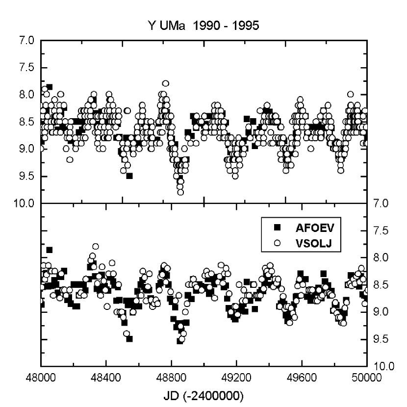
There are two steps in the data handling that precede before the period analysis: (1) data averaging using 10-day bins, and (2) merging of observations of different origin. We performed a few simple tests to decide whether merging should precede or follow the averaging. We plotted the different original light curves together for the best observed stars and found that the systematic differences did not exceed the level of the scatter in the data. One example can be seen in Fig. 1, where we have plotted the French and Japanese data for Y UMa (type SRb). The error of an individual point is estimated to be about mag. The two curves are very similar, which suggests that the comparison sequences define a well determined system of visual magnitudes. A similar conclusion was drawn for the majority of the stars in our sample, so we simply merged the available data before calculating the averaged curves. We could possibly reach somewhat better precision by introducing personal corrections for the most active observers, but as other tests have shown, the length of data is much more important in determining periodicities – which is our main goal – than is the accuracy of the individual measurements (see below). A thorough review of the homogeneity of visual photometry is given by Sterken & Manfroid (1992).
The averaging procedure consisted of taking 10-day bins and calculating the mean value from the individual points. Since the typical time scale of the period in our sample of semiregular variables is about one hundred days, this binning procedure does not smooth out significant detail in the light variations. A rough estimate of the resulting improvement in precision is as follows. As we mentioned earlier, the error of an individual observation is about mag. For a given 10-day bin with 10 points within it, the standard error of the mean value will be mag. The amount of data and their distribution in our sample in most cases permit such precision to be realized. Extremely deviant points differing from the mean value by more than were rejected in the original data during a close visual inspection of all light curves.
2.1 Tests of the quality and usability
Three tests were made to check the reliability and usability of the resulting mean light curves. The first was comparison with available simultaneous photoelectric V-measurements. Although the spectral response function of the human eye differs from the Johnson V filter, there were and continiue to be several attempts to find calibrations of transformations. Zissell (1998) modified the zeropoint of the conversion formula proposed by Stanton (1981) and gave the following relation:
According to the available photoelectric observations of semiregular variables, in most cases their colour changes with much smaller amplitude than V brightness does, thus it is a straightforward simplifying assumption that there is a constant shift between the photoelectric V and visual light curves. This is, of course, true only at a level of about 0.1 mag, which is in the range of the scatter of the visual data.
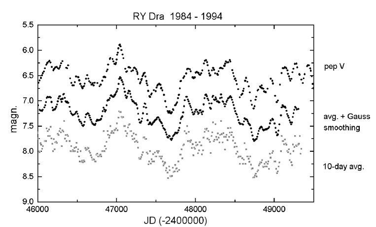
A direct comparison is shown in Fig. 2, where we compare visual data for RY Dra with simultaneous photoelectric V measurements carried out at Grinnel College. The top curve is the photoelectric one, while the bottom curve is the corresponding 10-day mean of visual data. The middle curve is a noise filtered version of the lower curve, where noise filtering was done by a simple Gaussian smoothing with 8 days FWHM. Note that while the visual curves were shifted in a vertical direction for clarity, the distance between the smoothed visual and the photoelectric curve is the real difference caused by the colour effects. The observed average shift of 0.60 mag is in good agreement with the predicted 0.57 mag by Eq. 1 ( for RY Dra). The agreement between the visual and photoelectric curves are very good, even the smallest humps and bumps, of 0.1 mag are clearly visible in the visual data. A similar conclusion can be drawn using Hipparcos Tycho V data (ESA 1997444http://astro.estec.esa.nl/Hipparcos): visual observations define light curves that are very similar to the photoelectric ones. We have to note, that the Gaussian data smoothing was applied only here because of its illustrative power, our main analyses were based on the 10-day binned light curves only.
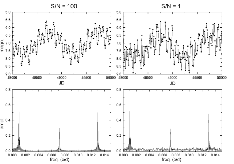
Another test was performed as a numerical simulation in order to study the effect of the length of the data set versus the signal-to-noise ratio (S/N). We generated artificial time-series by adding three monoperiodic signals with very similar periods and amplitudes to those observed in real variables (e.g. A mag, P days, A mag, P days, A mag, P days). Additional white noise was added to get artificial S/N values of 100 and 1, respectively. The “observed” time ranged from JD 2435000 to 2451000. We calculated the Discrete Fourier Transforms (DFT) for both datasets and the results are shown in Fig. 3.
It is obvious that the period (and amplitude) determination is almost completely independent of the S/N ratio if the time-series is long enough. This can be explained by the fact that the applied noise is independent of the current brightness and consequently these two quantities are also independent in the frequency domain. Real observations come from many different observers who made their estimates independently, therefore the observational noise is uncorrelated. We have extensively explored this question and our conclusion is that the analysed time-series fulfill all requirements for accurate period analysis. This result is similar to that of Szatmáry & Vinkó (1992). We have to note that the independence of noise and observations can be assumed only for bright semiregulars with amplitudes that are not too large. For Mira variables, which can become quite faint at minimum light, the data obtained by observers using small telescopes will have more scatter near the minima in the light curves.
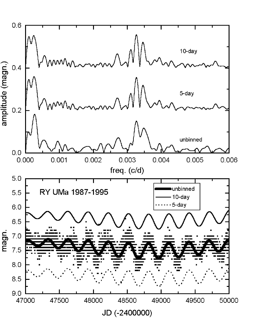
Following the referee’s note on using the averaged data, we have performed a third test addressed to the effects of the binning. The most important effect is the decrease of amplitude due to the binning, while the resulting frequencies may differ a bit, too. We explored this question by analysing the unbinned, 5-day and 10-day mean light curves.
| unbinned | 5-day | 10-day | |
|---|---|---|---|
| f0 | 0.000104 | 0.000100 | 0.000100 |
| A0 | 0.119 | 0.146 | 0.152 |
| f1 | 0.000272 | 0.000252 | 0.000248 |
| A1 | 0.178 | 0.170 | 0.165 |
| f2 | 0.003276 | 0.003276 | 0.003271 |
| A2 | 0.145 | 0.153 | 0.156 |
| f3 | 0.003500 | 0.003480 | 0.003480 |
| A3 | 0.119 | 0.108 | 0.113 |
The results of this test are briefly summarized in Fig. 4 with those of obtained for RY UMa (type SRb). We plotted three different Fourier-spectra calculated from the binned and original, unbinned data. The principal peaks have slightly different frequencies and amplitudes (Table 2), but the four-component fits (bottom panel in Fig. 4) do not differ significantly. This suggests that the differences are mainly due to the uncertainty of the whole analysis caused by the noisy data and not particularly due to the averaging. We conclude that the averaging procedure does not introduce significant alias structures, if the light curves are densely covered by many independent observations. We obtained similar results even for stars with periods of about 100 days (e.g. TX Dra) suggesting that data binning does not affect too seriously the calculated periods. The amplitudes have, of course, larger uncertainties, but as they may have cycle-to-cycle changes, this aspect is beyond our present scope.
3 Period analysis
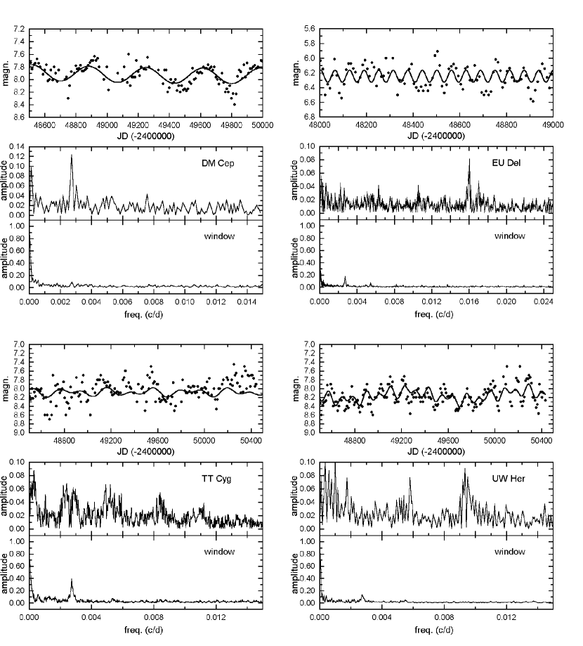
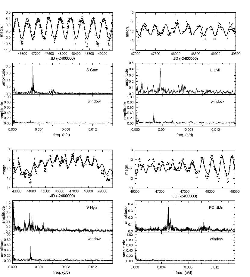
We calculated Discrete Fourier Transforms (DFT) of the merged and averaged time-series. The frequency ranged from 0 to 0.025 cycles/day, while the frequency step was chosen as c/d. The code used was Period98 (Sperl 1998555http://dsn.astro.univie.ac.at/period98). A few sample power spectra are presented in Figs. 5-6 and Sect. 4.
| Star | P (GCVS) | P | |||
|---|---|---|---|---|---|
| RV And | 10.0 | 22300 | 171 | 165(5) | 0.30 |
| S Aql | 10.5 | 25800 | 146 | 143(3) | 0.98 |
| GY Aql | 12.3 | 3000 | 204 | 464(4) | 2.35 |
| T Ari | 9.5 | 33000 | 317 | 320(3) | 0.91 |
| S Aur | 11.2 | 18800 | 590 | 596(6) | 0.61 |
| U Boo | 11.2 | 23300 | 201 | 204(3) | 0.62 |
| RV Boo | 8.5 | 7000 | 137 | 144(2) | 0.09 |
| S Cam | 9.3 | 28000 | 327 | 327(1) | 0.81 |
| RY Cam | 8.4 | 8500 | 136 | 134(1) | 0.16 |
| T Cnc | 9.0 | 12400 | 482 | 488(4) | 0.34 |
| RT Cap | 7.5 | 24000 | 393 | 400(4) | 0.31 |
| T Cen | 7.0 | 12400 | 90 | 91(1) | 0.62 |
| DM Cep | 7.9 | 6500 | – | 367(3) | 0.12 |
| RS CrB | 7.5 | 12400 | 322 | 331(1) | 0.19 |
| AI Cyg | 9.0 | 3000 | 197 | 146(2) | 0.18 |
| GY Cyg | 10.6 | 8000 | 300 | 143(1) | 0.13 |
| V460 Cyg | 6.5 | 6400 | 180 | 160(10) | 0.08 |
| V930 Cyg | 12.5 | 2000 | – | 247(3) | 0.72 |
| EU Del | 6.2 | 11000 | 60 | 62(1) | 0.08 |
| SW Gem | 8.8 | 11800 | 680 | 700(10) | 0.10 |
| RR Her | 9.0 | 27800 | 240 | 250(10) | 0.54 |
| RT Hya | 8.1 | 12400 | 290 | 255(3) | 0.20 |
| U Hya | 5.3 | 27800 | 450 | 791(5) | 0.06 |
| X Mon | 8.4 | 26600 | 156 | 148(7) | 0.59 |
| SY Per | 10.7 | 5000 | 474 | 477(9) | 0.89 |
| UZ Per | 8.7 | 4000 | 927 | 850(10) | 0.25 |
| W Tau | 10.4 | 24800 | 265 | 243(3) | 0.27 |
| V UMa | 10.4 | 12400 | 208 | 198(2) | 0.19 |
| SS Vir | 8.3 | 25500 | 364 | 361(1) | 0.81 |
There are some episodes in the light variation of RV And, S Aql and U Boo caused by possible mode switching (Cadmus et al. 1991).
We did not try to extract as many periods as possible from the power spectra because the excited frequencies in semiregular variables are not stable over time (see, e.g., Mattei et al. 1998). The DFT may contain many misleading peaks because of the cycle-to-cycle variations. These changes make impossible to fit simple sums of sines. Our approach was to accept only the most dominant periods which were tested by whitening, cleaning and alias filtering. One-year alias peaks occur for many stars, while in some cases cross production terms are present as well (e.g. ). We did an iterative period determination allowed by Period98 (Sperl 1998), in which we checked the consistency of the fitted harmonics and the light curve itself after every step. The frequency identification was a quite difficult task in certain stars (e.g. TT Cyg, TZ Cyg and other low-amplitude variables), mainly because of the long-term changes in the mean brightness. They may cause fairly high false peaks in the low-frequency region which have to be subtracted and neglected in searching for pulsational periods. This involves some additional uncertainty which can be hardly avoided. The instabilities of the excited frequencies may cause multiple peaks scattering around local average values in the Fourier spectra, therefore, in some cases (TT Cyg, X Her, TZ Cyg, SW Gem, U Hya, S Sct, SW Vir) we could only estimate the periods and amplitudes with help of a paralel comparison of the multiple structures of the DFT and the observed cyclic changes in the light curves. The determined “periods” in the quoted stars should be rather considered as characteristic times of variations instead of real periods.
The resulting periodicities can be summarized as follows. Among the 93 semiregulars, we have found 29 purely monoperiodic stars, 56 stars with unambiguous multiperiodic behaviour (44 bi- and 12 triperiodic), and 8 stars which turned out to be rather irregular (meaning that we did not find any peak higher than the calculated noise level for those variables). We present the main observational properties (average brightness, length of analysed data in days) as well as the calculated periods and their amplitudes in Tables 3–5. The period uncertainty was estimated from the width of the peaks in the spectra at 90% of maximum. One star, RS Cam, apparently has a fourth period ( days, mag.) as well. The amplitude values have more uncertainty than do the periods because of the instability of the periods. This issue was studied by wavelet analysis (see Sect. 4 for examples), which is a useful tool for studying temporal variations in the frequency content (see, e.g., Bedding et al. 1998, Barthés & Mattei 1997, Szatmáry et al. 1996, Foster 1996, Gál & Szatmáry 1995a, Szatmáry et al. 1994, Kolláth & Szeidl 1993, Szatmáry & Vinkó 1992). Therefore, the amplitude values listed in Tables 3–5 only serve to indicate the approximate relative strengths of the corresponding periods.
| Star | P (GCVS) | ||||||
|---|---|---|---|---|---|---|---|
| ST And | 10.0 | 5300 | 328 | 338(2) | 1.15 | 181(1) | 0.20 |
| VX And | 8.5 | 5800 | 369 | 904(5) | 0.16 | 375(2) | 0.27 |
| AQ And | 8.6 | 8200 | 346 | 346(1) | 0.15 | 169(1) | 0.18 |
| V Aqr | 8.7 | 22800 | 244 | 689(5) | 0.25 | 241(2) | 0.35 |
| V Aql | 7.4 | 28300 | 353 | 400(50) | 0.10 | 215(1) | 0.11 |
| RS Aur | 10.0 | 22300 | 170 | 173(1) | 0.29 | 168(1) | 0.23 |
| UU Aur | 5.7 | 21800 | 234 | 441(2) | 0.15 | 235(2) | 0.09 |
| V Boo | 8.7 | 27800 | 258 | 257(1) | 0.86 | 137(1) | 0.19 |
| RR Cam | 10.5 | 12400 | 124 | 223(2) | 0.09 | 124(1) | 0.10 |
| V CVn | 7.5 | 26400 | 192 | 194(1) | 0.42 | 186(1) | 0.13 |
| SV Cas | 8.6 | 25000 | 265 | 460(4) | 0.48 | 262(2) | 0.32 |
| WZ Cas | 7.2 | 11000 | 186 | 373(1) | 0.16 | 187(1) | 0.09 |
| SS Cep | 7.3 | 27000 | 90 | 340(10) | 0.07 | 100(5) | 0.05 |
| W Cyg | 6.2 | 33400 | 131 | 240(5) | 0.05 | 130(5) | 0.14 |
| RS Cyg | 8.0 | 27800 | 417 | 422(4) | 0.48 | 211(2) | 0.20 |
| RU Cyg | 8.5 | 26800 | 233 | 441(1) | 0.16 | 234(1) | 0.96 |
| RZ Cyg | 11.8 | 28800 | 276 | 537(2) | 0.63 | 271(4) | 0.86 |
| TT Cyg | 8.0 | 25500 | 118 | 390(10) | 0.03 | 188(5) | 0.03 |
| TZ Cyg | 10.8 | 9500 | – | 138(1) | 0.06 | 79(1) | 0.05 |
| AB Cyg | 7.9 | 25400 | 520 | 513(2) | 0.17 | 429(2) | 0.07 |
| AW Cyg | 8.9 | 22300 | 340 | 3700(50) | 0.10 | 387(3) | 0.10 |
| U Del | 7.0 | 29800 | 110 | 1146(10) | 0.21 | 580(5) | 0.05 |
| S Dra | 8.9 | 26600 | 136 | 311(1) | 0.12 | 172(2) | 0.12 |
| RY Dra | 7.0 | 8800 | 200 | 1150(20) | 0.20 | 300(10) | 0.10 |
| UX Dra | 6.7 | 8000 | 168 | 317(2) | 0.08 | 176(1) | 0.10 |
| AH Dra | 7.8 | 8600 | 158 | 189(1) | 0.25 | 107(1) | 0.12 |
| RS Gem | 10.6 | 12400 | 140 | 271(1) | 0.25 | 148(1) | 0.22 |
| X Her | 6.7 | 33500 | 95 | 178(5) | 0.05 | 102(5) | 0.03 |
| ST Her | 7.9 | 25000 | 148 | 263(2) | 0.08 | 149(1) | 0.08 |
| g Her | 5.1 | 9000 | 89 | 887(5) | 0.20 | 90(1) | 0.07 |
| V Hya | 9.1 | 32600 | 531 | 6400(50) | 1.22 | 531(3) | 0.66 |
| RY Leo | 10.2 | 22000 | 155 | 160(1) | 0.40 | 145(1) | 0.28 |
| U LMi | 11.8 | 10000 | 272 | 272(2) | 0.45 | 144(1) | 0.16 |
| W Ori | 6.5 | 33300 | 212 | 2390(20) | 0.15 | 208(1) | 0.08 |
| BQ Ori | 7.9 | 26000 | 110 | 240(6) | 0.14 | 127(2) | 0.10 |
| Y Per | 9.4 | 24000 | 249 | 245(1) | 0.36 | 127(1) | 0.16 |
| S Sct | 7.3 | 22400 | 148 | 269(5) | 0.08 | 149(2) | 0.10 |
| Ser | 6.7 | 5800 | 100 | 1240(10) | 0.10 | 111(1) | 0.09 |
| Y Tau | 7.4 | 27000 | 242 | 461(2) | 0.18 | 242(1) | 0.18 |
| Z UMa | 7.8 | 31000 | 196 | 195(1) | 0.33 | 100(1) | 0.05 |
| RY UMa | 7.3 | 9800 | 310 | 305(1) | 0.16 | 287(1) | 0.11 |
| ST UMa | 6.8 | 26000 | 110 | 5300(20) | 0.11 | 615(6) | 0.09 |
| R UMi | 9.7 | 28000 | 326 | 325(1) | 0.42 | 170(1) | 0.11 |
| RU Vul | 9.3 | 19500 | 174 | 369(2) | 0.13 | 136(1) | 0.11 |
| Star | P (GCVS) | ||||||||
|---|---|---|---|---|---|---|---|---|---|
| U Cam | 8.2 | 26800 | – | 2800(100) | 0.13 | 400(30) | 0.09 | 220(5) | 0.09 |
| RS Cam | 8.7 | 25000 | 89 | 966(10) | 0.17 | 160(1) | 0.15 | 90(1) | 0.12 |
| ST Cam | 7.3 | 28000 | 300 | 1580(10) | 0.10 | 372(3) | 0.12 | 202(2) | 0.08 |
| X Cnc | 6.7 | 25800 | 195 | 1870(10) | 0.08 | 350(3) | 0.08 | 193(1) | 0.09 |
| Y CVn | 5.7 | 28500 | 157 | 3000(100) | 0.08 | 273(3) | 0.06 | 160(2) | 0.05 |
| AF Cyg | 7.2 | 26600 | 93 | 921(10) | 0.08 | 163(1) | 0.11 | 93(1) | 0.11 |
| TX Dra | 7.6 | 26800 | 78 | 706(2) | 0.10 | 137(1) | 0.06 | 77(3) | 0.07 |
| UW Her | 8.1 | 8600 | 104 | 1000(10) | 0.09 | 172(1) | 0.08 | 107(1) | 0.09 |
| Y UMa | 8.6 | 32000 | 168 | 324(1) | 0.16 | 315(1) | 0.09 | 164(2) | 0.06 |
| RX UMa | 10.6 | 33200 | 195 | 201(1) | 0.37 | 189(1) | 0.26 | 98(0.5) | 0.16 |
| V UMi | 8.1 | 29000 | 72 | 737(10) | 0.06 | 126(2) | 0.04 | 73(0.5) | 0.06 |
| SW Vir | 7.6 | 8500 | 150 | 1700(50) | 0.15 | 164(1) | 0.13 | 154(1) | 0.20 |
3.1 Discussion of the multiperiodic nature
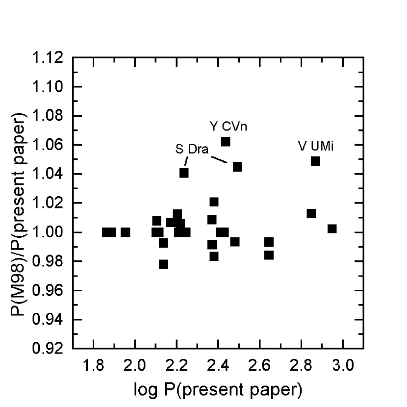
Mattei et al. (1998, hereafter M98) found 30 semiregular variables with two periods. Our periods for the 16 common stars are in very good agreement. This is also true for the two triply periodic variables, V UMi and TX Dra. Since the semiregulars have quite noisy light curves due to the intrinsic short-timescale structure, it is worth comparing the independently determined periodicities by plotting period ratios against our periods (Fig. 7). The significantly deviant points are those of V UMi, Y CVn and S Dra. This can be explained by the instability of the periods and the different length of the analysed data in M98. The time span of the dataset studied here is more than twice that of M98. Because the period and amplitude may be changing over time, the results obtained with datasets covering different time spans will be different. Thus, we conclude that the applied period determination and alias filtering give consistent results with the earlier independent study.
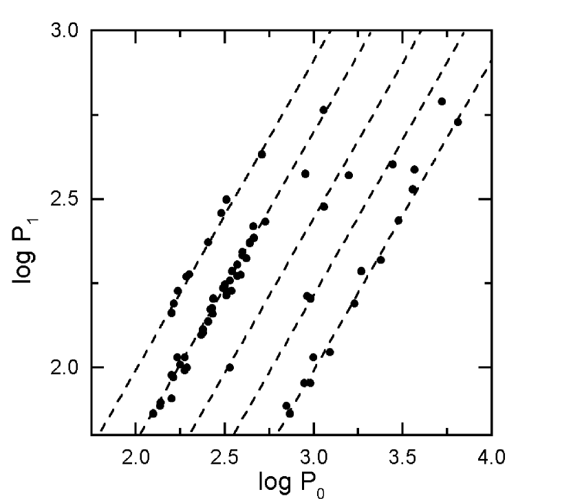
In order to examine the general distribution of the periods, we made pairs of periods in 56 multiperiodic variables. This was done in triply periodic stars by sorting the periods and choosing the two neighbouring values. Shorter periods against the longer ones are plotted in Fig. 8. Three sequences are clearly present while two others are suggested. All of them are marked by dashed lines that were drawn by fitting a least-squares linear trend to the most populated sequence and shifting that line to match the other sequences. It is very interesting how parallel these ridges of data points are. One would expect such a separation between stars pulsating in different modes (i.e., for the same “longer” period value different “shorter” periods correspond), assuming that the periodicities are due to pulsation.
Since pulsation theory usually uses period ratios to predict the modes, we plotted the Petersen diagram (period ratios vs. periods) in Fig. 9. The most populated region contains stars with period ratios between 1.80 and 2.00, while the other sequences are those of with ratios of around 10–12, 6.0, 3.60–3.90 and 1.02–1.10. Mattei et al. (1998) pointed out that in their sample 63% (19 of 30) of the multiperiodic stars have period ratios between 1.80 and 2.00. Our larger sample supports this statistic, as 39 of 56 stars (70%) have period ratios of around . The dashed lines in Fig. 9 were fitted by the same procedure as in Fig. 8.
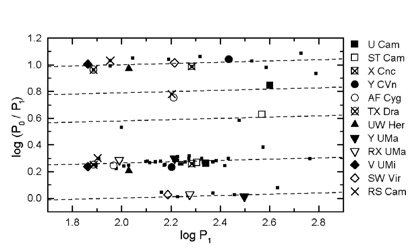
The other period ratios are interesting, too. The lowest sequence is that of stars with period ratios somewhat higher than 1. This means two closely separated periods, assuming that the close peaks are not due to small changes of one period. We have checked the original light curves and found very clear examples for beating (e.g. RU And, RX UMa). On the other hand, some stars should be considered as monoperiodic variables with slightly and randomly changing period. Unfortunately, it is very difficult to distinguish between these possibilities. The upper sequence in Fig. 9 is populated by stars with period ratios of around 10. This is a well-known period ratio for semiregulars (e.g. Houk 1963, Wood 1976, Percy & Polano 1998). The intermediate ratios were not discussed in the earlier papers, although they are present in their observational analyses to a smaller extent (see Fig. 6 in M98).
The assumption of a few simultaneously excited modes can be tested by the triply-periodic variables. If their period ratios fall on the sequences defined by the doubly periodic stars that would support the assumption. Fig. 9 shows those stars separately. The main sequences are evidently well covered by the triply-periodic semiregulars only, too. Most recently, Bedding et al. (1998) have studied the mode switching in R Dor () concluding that it probably pulsates in the first and third overtones. Furthermore, they suggest that all stars with similar period ratios pulsate in these modes. Wood et al. (1998) presented multiple structures in a diagram similar to Fig. 8 for the LMC red variables, and also suggested higher modes than fundamental and first overtone.
Although Figs. 8–9 supports the idea that the segregation is a consequence of the presence of many modes of pulsation, other possible explanations could not be excluded. Older models by Fox & Wood (1982) predict high period ratios (6–10) for masses as high as 6–8 , while the periods of fundamental and first overtone radial modes have ratios of about 2 in many theoretical models (e.g. Ostlie & Cox 1986, Fox & Wood 1982). On the other hand, quasi-periodic cycles might be caused by physical mechanisms other than pulsation (e.g. duplicity, distorted stellar shapes, rotation – Barnbaum et al. 1995, dust-shell dynamics – Höfner et al. 1995). Nevertheless, we can claim that: i) a significant percentage of semiregular stars show multiperiodic behaviour; ii) there is supporting evidence provided by the triply periodic variables that the segregation in Figs. 8–9 is due to different modes of pulsation.
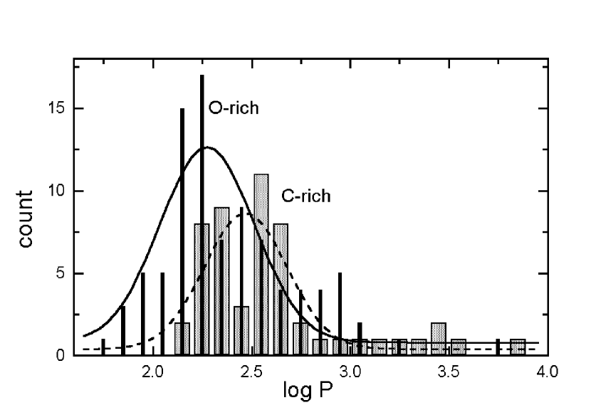
We have tried to find correlations among the periods, the period ratios, and several main physical properties, such as the infrared JHKL’M colours (Kerschbaum & Hron 1994), galactic latitude, and mass-loss rates (Loup et al. 1993). No correlation was found among these parameters. We have also tried to find a distinction between the C-rich and O-rich variables, but the photometric parameters studied did not allow to determine such a discrimination. Nevertheless, we plotted the period distribution of the two types of stars in Fig. 10. This diagram is strongly biased by the effects of the sample selection, as noted by the referee: long-period O-rich stars would have on the average larger amplitudes (due to the O-rich opacity sources, such as VO, TiO), and would be classified as Miras and consequently not enter the sample. Visual C-rich stars with small amplitudes have on the average higher luminosities and therefore longer periods. The simple Gaussian fits marked by the solid and dashed lines were used to estimate the maximum and the spread of the distributions (186 and 295 days for O-rich and C-rich stars, respectively; the FWHM is 0.440.07 dex for both fits).
4 Special cases
This section deals with examples illustrating our analysis procedure and the application of wavelet analysis. The stars mentioned below as well all other stars will be investigated in more details in a subsequent paper. Here we briefly outline only what we found especially interesting. The examples cover triple periodicity (TX Dra and V UMi), amplitude modulation (RY UMa) and long-term amplitude decrease (V Boo, RU Cyg and Y Per).
4.1 TX Draconis & V Ursae Minoris
The clearest examples of triple periodicity are TX Dra and V UMi. In many respects they are twins in their pulsational characteristics. The dominant modes of TX Dra and V UMi have periods of 77 days and 73 days, respectively. The other periods are also very similar: 706 and 137 days for TX Dra versus 737 and 126 days for V UMi. This result is in perfect agreement with that of Mattei et al. (1998), except for the longest period in V UMi. This can be explained by the instability of this period which caused a double peak around 750 days in the Fourier spectrum with slightly differing amplitudes. These peaks correspond exactly to our 73710 days and M98’s 773 days periods. The data distribution is not the same in the two analysed data sets which affected the calculated amplitudes.
We studied the stability of the frequency content by wavelet analysis (e.g. Szatmáry et al. 1996, Foster 1996, Szatmáry et al. 1994). The resulting three-dimensional wavelet contour maps and the corresponding Fourier spectra are shown in Figs. 11-12. The most unstable period in TX Dra is the shortest one (77 days). While the other two modes seem to be quite stable over thousands of days, the short period component sometimes switches on and off. That is why there are many peaks in the power spectrum scattering around the average value of 77 days. Observers should note that the dominant mode is, as of February 1999, this rapid one, and based on earlier behaviour, we expect that it will switch off around 1999–2000, thereby offering a very good opportunity to observe mode switching in real-time!
V UMi is generally very similar to TX Dra, even in the instability of the excited modes. Obviously the pulsation in these stars is not a smooth and repetitive process. Mild chaos is probably present, too, as suggested by, e.g., Mattei et al. (1998). The extended atmosphere with strong inner convection creates a very complex environment where slight changes in the actual parameters have very serious effects on the resulting pulsational properties.
The change between pulsational modes has been detected in the case of some 53 Per stars (Smith 1978), in a rapidly oscillating Ap star (Kreidl et al. 1991), and in F supergiant (Fernie 1983). Mode switching in red semiregular stars was reported by Cadmus et al. (1991), Gál & Szatmáry (1995b), and Percy & Desjardins (1996). Further cases of mode switching and models for this phenomenon are discussed by Bedding et al. (1998).
4.2 RY Ursae Majoris
Amplitude modulation in pulsating variables is mainly associated with RR Lyrae variables showing the Blazhko-effect (e.g. Kovács 1995, Szeidl 1988, Moskalik 1986), with Scuti-type stars with very complex light variations (e.g. Mantegazza et al. 1996, Breger 1993), one known classical Cepheid, V473 Lyr, which has strong amplitude modulation (Van Hoolst & Waelkens 1995), and some Mira and semiregular variables (Mattei 1993, Mattei et al. 1998, Mattei & Foster 1999a, b, Barthés & Mattei 1997).
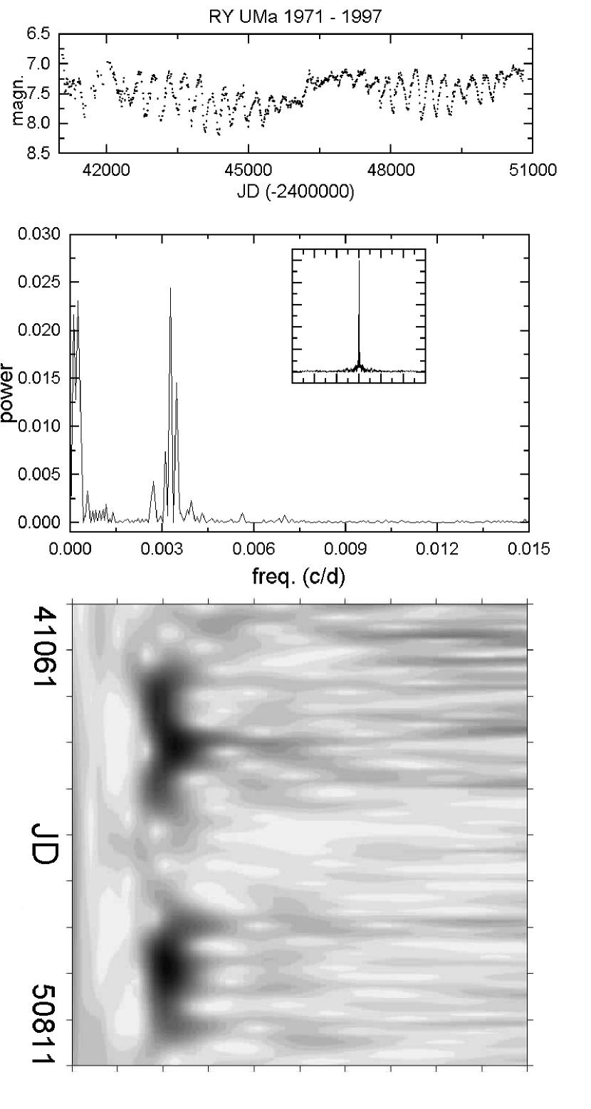
In our sample, one of the best examples of semiregular variables with amplitude modulation is RY UMa, which is classified as an SRb star. Its light curve reveals a clear amplitude modulation which is strongly supported by the results of wavelet analysis (Fig. 13). Although the Fourier spectrum suggests two closely separated periods (see Table 4), accepting them would be misleading, as the wavelet map shows slight frequency changes of the principal peak accompanied with amplitude modulation. Therefore, that close peak is an artifact caused by the instability of the principal one. The underlying physical mechanism in unknown: there are several possibilities such as the rotation, magnetic activity change or duplicity effects. Unfortunately the presently available observations do not allow finding a reliable model for this modulation. Nevertheless, it is very interesting that the characteristic time of the amplitude modulation is about 4000 days being around a typical value of theoretically calculated rate of rotation of red giant stars (as estimated using rotational velocities studied by Schrijver & Pols 1993).
4.3 V Bootis, RU Cygni & Y Persei
V Boo is the prototype of SRa variables suffering from long-term amplitude decrease (Szatmáry et al. 1996). Recently Bedding et al. (1998) presented a very similar phenomenon for R Dor which was classified in GCVS as an SRb star. The proposed explanation for the amplitude decrease in R Dor is that the star is evolving from the Mira state to the semiregular state. We found another two examples of amplitude decrease in RU Cyg (SRa) and Y Per (Mira), which are consequently the third and fourth candidates for that interesting evolutionary status. Unfortunately, these substantial changes of the lightcurves are only hints of probable change of the variability type, further spectroscopic or near-infrared photometric observations would be desirable. V Boo and RU Cyg are compared in Fig. 14, where long-term light curves are plotted together with the corresponding power spectra and wavelet maps. The similarity is quite conspicuous.
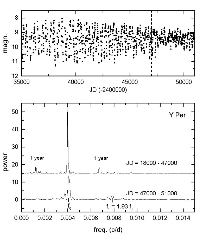
Y Per differs from V Boo and RU Cyg in a very important aspect. While the dominant frequencies of V Boo and RU Cyg did not change significantly, Y Per seems to be a clear example of a transition from Mira to SRb. This is presented in Fig. 15, where the compressed light curve is plotted with two power spectra corresponding to two data subsets (before and after JD 47000). The earlier monoperiodicity (P=253 day) was replaced by a biperiodicity (P0=245 day, P1=127 day). Apparently the Mira star Y Per was transformed to a typical doubly-periodic SRb star. The most surprising result is the abruptness of the mode switching.
5 Summary
Based on the light curve analyses presented in the previous sections we have obtained the following results:
1. We have analysed long-term visual observations of 93 red semiregular variables in order to determine their dominant periods. Direct comparison with photoelectric measurements demonstrated the usefulness of the low quality visual data. The most important requirement of precise frequency determination is to have as long a time-series as possible, as has been illustrated by frequency analysis of artificial data.
2. We have found 29 monoperiodic and 56 multiperiodic stars (44 with two and 12 with three significant and essentially stable periods). 8 variables do not show any unambiguous periodicity. The distribution of periods and period ratios in multiperiodic variables suggests the existence of up to five different groups among the variables studied, which is most probably due to different modes of pulsation.
3. We have highlighted a few interesting special cases:
-
•
TX Dra and V UMi are very similar triply-periodic variables with nearly equal periods. While the longer two periods are stable over decades of time, the high-frequency mode switches on and off from time to time. We predict another mode change of TX Dra soon, most probably in 1999-2000.
-
•
RY UMa is one of the best documented examples for amplitude modulation in SRV’s. Unfortunately the visual data alone are not enough to determine the underlying physical process.
-
•
We have discussed three stars (V Boo, RU Cyg and Y Per) that show a gradual decrease in amplitude. All of them seem to evolve from mira-like to semiregular type (as does R Dor, according to Bedding et al. 1998), which suggests that Miras and SRV’s may be much more closely related than was thought earlier. Y Per differs from the other stars, because, in addition to the amplitude decrease, a new mode has appeared with a quite high amplitude. The observed period ratio (1.93) is very typical in the majority of doubly periodic SRV’s.
Acknowledgements.
We sincerely thank variable star observers of AFOEV, VSOLJ, HAA/VSS and AAVSO whose dedicated observations over many decades made this study possible. The referee (Dr. F. Kerschbaum) has greatly improved the paper with his notes and suggestions. This research was supported by Hungarian OTKA Grants #F022249, #T022259 and Szeged Observatory Foundation. The NASA ADS Abstract Service was used to access data and references.References
- (1) Alves, D. et al. (The MACHO Collaboration) 1998, in: “Pulsating Stars - Recent Developments in Theory and Observations”, eds. M. Takeuti & D.D. Sasselov, Universal Academy Press, Tokyo, p.17
- (2) Andronov, I.L. 1998, poster P2-01 on IAU Symp. 191 “AGB Stars”, Montpellier, France
- (3) Barnbaum, C., Morris, M., Kahane, C. 1995, ApJ 450, 862
- (4) Barthés, D. & Mattei, J.A. 1997, AJ 113, 373
- (5) Bedding, T.R. & Zijlstra, A.A. 1998, ApJ 506, L47
- (6) Bedding, T.R., Zijlstra, A.A., Jones, A., Foster, G. 1998, MNRAS 301, 1073
- (7) Breger, M. 1993, Ap&SS 210, 173
- (8) Cadmus, Jr., R. R., Willson, L. A., Sneden, C., Mattei, J. A. 1991, AJ 101, 1043
- (9) Cook, K.H. et al. 1997, in the Proceedings of the 12th IAP Colloquium, Variable Stars and the Astrophysical Returns of Microlensing Surveys, 17
- (10) Fernie, J. D. 1983, ApJ 265, 999
- (11) Foster, G. 1996, AJ 112, 1709
- (12) Fox, M.W. & Wood, P.R. 1982, ApJ 259, 198
- (13) Gál, J. & Szatmáry, K. 1995a, A&A 297, 461
- (14) Gál, J. & Szatmáry, K. 1995b, in: “Astrophysical Applications of Stellar Pulsation”, eds. R. S. Stobie, P. A. Whitelock, ASP Conference Series, Vol. 83, p. 405
- (15) Höfner, S., Feuchtinger, M.U., Dorfi, E.A. 1995, A&A 297, 815
- (16) Hron, J., Aringer, B., Kerschbaum, F. 1997, A&A 322, 280
- (17) Houk, N. 1963, AJ 68, 253
- (18) Jura, M. & Kleinmann, S.G. 1992, ApJSS 83, 329
- (19) Kerschbaum, F. & Hron, J. 1992, A&A 263, 97
- (20) Kerschbaum, F. & Hron, J. 1994, A&AS 106, 397
- (21) Kerschbaum, F. & Hron, J. 1996, A&A 308, 489
- (22) Kerschbaum, F. & Olofsson, H. 1998, A&A 336, 654
- (23) Kerschbaum, F., Lazaro, C., Habison, P. 1996, A&AS 118, 397
- (24) Kolláth, Z. & Szeidl, B. 1993, A&A 277, 62
- (25) Kovács, G. 1995, A&A 295, 693
- (26) Kreidl, T. J., Kurtz, D. W., Bus, S. J., Kuschnig, R., Birch, P. B., Candy, M. P., Weiss, W. W. 1991, MNRAS 250, 447
- (27) Lebzelter, T., Kerschbaum, F., Hron, J. 1995, A&A 298, 159
- (28) Loup, C., Forveille, T., Omont, A., Paul, J.F. 1993, A&AS 99, 291
- (29) Mantegazza, L., Poretti, E., Bossi, M. 1996, A&A 308, 847
- (30) Mattei, J.A. 1993, J. Amer. Assoc. Var. Star Obs. 22, 47
- (31) Mattei, J.A., Foster, G., Hurwitz, L.A., Malatesta, K.H., Willson, L.A., Mennessier, M.O. 1998, in the Proceedings of the ESA Symposium “Hipparcos - Venice’97”, ESA SP-402, p.269
- (32) Mattei, J.A. & Foster, G. 1999a, in “Carbon Star Phenomena”, ed. R. Wing, Kluwer Academic Publishers, Dordrecht, in press
- (33) Mattei, J.A. & Foster, H. 1999b, in “Variable Stars as Important Astrophysical Tools”, ed. C. Ibanoglu, Kluwer Academic Publishers, Dordrecht, in press
- (34) Minitti, D. et al. (The MACHO Collaboration) 1998, in: “Pulsating Stars - Recent Developments in Theory and Observations”, eds. M. Takeuti & D.D. Sasselov, Universal Academy Press, Tokyo, p.5
- (35) Moskalik, P. 1986, Acta Astr. 36, 333
- (36) Ostlie, D.A., Cox, A.N. 1986, ApJ 311, 864
- (37) Percy, J.R., Ralli, J.A., Sen, L.V. 1993, PASP 105, 287
- (38) Percy, J.R., Desjardins, A. 1996, PASP 108, 847
- (39) Percy, J.R. & Polano, S. 1998, ASP Conf. Series, 135, 249
- (40) Schrijver, C.J. & Pols, O.R. 1993, A&A 278, 51
- (41) Smith, M. A. 1978, ApJ 224, 927
- (42) Sperl, M. 1998, Comm. Astr. Seis. 111
- (43) Sterken, C. & Manfroid, J. 1992, in: “Variable Star Research: An International Perspective”, eds. J.R. Percy, J.A. Mattei, C. Sterken, Cambridge Univ. Press, Cambridge, p.75
- (44) Stanton, R.H. 1981, J. Amer. Assoc. Var. Star Obs., 10, 1
- (45) Szatmáry, K., Vinkó, J. 1992, MNRAS, 256, 321
- (46) Szatmáry, K., Vinkó, J., Gál, J. 1994, A&AS, 108, 377
- (47) Szatmáry, K., Gál, J., Kiss, L.L. 1996, A&A, 308, 791
- (48) Szeidl, B. 1988, in: “Multimode Stellar Pulsations”, eds. G. Kovács, L. Szabados, B. Szeidl, Konkoly-Kultura, Budapest, p.45
- (49) Van Hoolst, T., Waelkens, C., 1995, A&A, 295, 361
- (50) Welch, D.L. 1998, ASP Conf. Series, 135, 355
- (51) Wood, P. 1976, in: “Multiple Periodic Variable Stars”, ed. W.S. Fitch, Akadémiai Kiadó, Budapest, p.69
- (52) Wood, P. et al. (The MACHO Collaboration) 1998, IAU Symp. 191 “AGB Stars”, Montpellier, France
- (53) Zissell, R. 1998, J. Amer. Assoc. Var. Star Obs., 26, 151