Scaling laws in gravitational clustering for counts-in-cells and mass functions
Abstract
We present in this article an analysis of some of the properties of the density field realized in numerical simulations for power-law initial power-spectra in the case of a critical density universe. We study the non-linear regime, which is the most difficult to handle analytically, and we compare our numerical results with the predictions of a specific hierarchical clustering scaling model that have been made recently, focusing specifically on its much wider range of applicability, which is one of its main advantages over the standard Press-Schechter approximation. We first check that the two-point correlation functions, measured both from counts in cells and neighbour counts, agree with the known analytically exact scaling requirement (i.e. only depend on ) and we also find the stable-clustering hypothesis to hold. Next we show that the statistics of the counts in cells obey the scaling law predicted by the above scaling model.
Then we turn to mass functions of overdense and underdense regions, that we obtain numerically from “spherical overdensity” and “friends-of-friends” algorithms. We first consider the mass function of “just-collapsed” objects defined by a density threshold and we note as was found by previous studies that the usual Press-Schechter prescription agrees reasonably well with the simulations (although there are some discrepancies). On the other hand, the numerical results are also consistent with the predictions of the scaling model. Then, we consider more general mass functions (needed to describe for instance galaxies or Lyman- absorbers) defined by different density thresholds, which can even be negative. The scaling model is especially suited to account for such cases, which are out of reach of the Press-Schechter approach, and it still shows reasonably good agreement with the numerical results. Finally, we show that mass functions defined by a condition on the radius of the objects also satisfy the theoretical scaling predictions.
Thus, we find that the scaling model provides a reasonable description of the density field in the highly non-linear regime, for the cosmologies we have considered, both for the counts in cells statistics and the mass functions. The advantages of this approach are that it clarifies the links between several statistical tools and it allows one to study many different classes of objects, for any density threshold, provided one is in the fully non-linear regime.
keywords:
Cosmology: theory - large-scale structure of Universe - galaxies : clustering1 Introduction
In the standard cosmological scenario large-scale structures in the universe arise from the amplification through gravitational instability of small primordial density fluctuations. These initial perturbations are likely to be gaussian (as in most inflationary models) and are characterized by their power-spectrum. Within the hierarchical clustering scenario, the amplitude of these fluctuations increases towards the smaller scales (as in the CDM model: Peebles 1982; Davis et al.1985). Small scales collapse first to form bound objects which merge later to build increasingly massive halos as larger scales become non-linear. These mass condensations correspond to the various astrophysical objects one can observe in the universe, from Lyman- clouds to galaxies and clusters. As a consequence, to understand the formation of these objects it is important to obtain a precise description of the evolution of the density field under the action of gravity. Note that to model specific astrophysical objects one usually needs to add to this description of dark matter halos non-gravitational effects (such as, for instance, radiative processes to get the evolution of baryons). This is beyond the scope of the present paper that considers specifically the multiplicity of dark halos.
However, even for the problem of the evolution of the matter distribution under the sole action of gravity theoretical results are very scarce. Linear theory allows one to describe the density field on large scales, while a few approximations (e.g. see Bernardeau 1996) try to handle the early non-linear evolution, but the highly non-linear regime has proved very difficult to model. As a consequence numerical simulations have so far been the main tool to describe this latter stage. In this article, we compare the results of simulations for power-law initial spectra in the case of a critical density universe with the scaling model presented in previous publications (Valageas & Schaeffer 1997, hereafter VS; Bernardeau and Schaeffer 1991; Balian & Schaeffer 1989a ). This latter description of the density field is based on the assumption that the many-body correlation functions satisfy specific scaling laws (obtained from the stable-clustering ansatz) in the highly non-linear regime. In this case one obtains a very powerful model for the density field, which can be used to obtain the counts in cells statistics as well as mass functions of overdense and underdense regions at different density thresholds. Note that in contrast the Press-Schechter (PS) mass function (Press & Schechter 1974), which is certainly the most popular tool to get some information on the characteristics of the non-linear density field, only deals with “just-collapsed” objects.
The article is organized as follows. In Sect.2 we describe the numerical simulations we analyse. Then we present our results for the two-point correlation function and the counts in cells statistics in Sect.3. We compare the numerical mass function of “just-collapsed” objects to the usual PS prescription and to the scaling model in Sect.4. We also consider more general mass functions, beyond the reach of the PS approach, that are defined by various density thresholds. Finally we present our results for the limiting case of mass functions of objects defined by a constant radius constraint. These studies originate from astrophysical descriptions of galaxies (Valageas & Schaeffer 1999; Valageas & Silk 1999) and Lyman- clouds (Valageas et al.1999) where one is naturally led to introduce such generalized mass functions.
2 Simulations
We shall consider a critical density universe, , with an initial power-spectrum which is a power-law: . We study the cases , and . As usual we shall define to be the amplitude of the density fluctuations in cells of physical radius at time (scale-factor ) given by linear theory. Thus we have:
| (1) |
where is a comoving scale.
The N-body simulations were performed using the code of Couchman (1991). The nominal box size was Mpc/h (though this could be rescaled to any value, since the initial conditions are scale-free). The simulations all used particles, with a force-softening parameter (constant in comoving coordinates) of times the mean interparticle separation , that is over a comoving radius of Mpc/h. The expansion factor was normalized so that for Mpc/h at , according to linear theory. The initial positions and velocities of the particles were given by displacing the particles from a cubical grid using the Zeldovich approximation and the linear theory power spectrum. The starting time was chosen small enough so that the density fluctuations on the scale of the particle grid were still close to the linear regime. Specifically, the linear power-spectrum amplitude at the Nyquist frequency of the particle grid was chosen to be times the white noise value, with for and , and for , corresponding to expansion factors for respectively. For , the simulation was evolved with a constant timestep in the variable , while for and a constant timestep in was used, with respectively. The simulations were evolved up to expansion factors for respectively. In the numerical analysis we shall use the output times in the range when some non-linear structures have already formed on scales larger than the smoothening length.
For this cosmology and initial power spectra, the real clustering evolution should be self-similar, when scaled to a radius such that . This is an exact analytical result that holds independently of the validity of the Balian & Schaeffer (1989a ) scaling predictions (see Sect.3) that we aim at testing in this paper. The evolution in the N-body simulation will depart from exact self-similarity because of numerical effects, in particular, particle discreteness, force softening, the finite box size, and the absence of initial fluctuations smaller than the Nyquist wavelength or larger than the box size.
3 Counts-in-cells
A convenient way to describe the density field obtained in a numerical simulation, or realized in the actual universe, is to consider the counts in cells. Thus, we define the probability distribution to be the probability to have particles in a spherical cell of radius at a given time . In the following we shall usually denote as to simplify the notation. This is a well-defined quantity which provides a very good description of the density field and is a convenient tool for a theoretical analysis. In contrast, the multiplicity functions used to recover the counts of virialized halos or astrophysical objects may be defined in various ways and are somewhat more difficult to handle analytically. However, in certain regimes their properties can be obtained from the characteristics of the counts in cells. Hence we shall first consider the statistics of in the next sections.
3.1 Non-linear scaling model
Since we shall mainly compare our results with the scaling model described in Balian & Schaeffer (1989a ) we recall here their predictions while introducing our notation. This model is based on the assumption that the many-body correlation functions satisfy the scaling law :
| (2) |
where is the scale-factor and is the slope of the two-point correlation function (which we note ). For an initial power-spectrum which is a power-law, , we have:
| (3) |
The relations (2) and (3) are derived from the stable-clustering assumption (Davis & Peebles 1977; Peebles 1980) and are expected to describe the highly non-linear regime . To obtain the statistics of in cells of radius , volume , it is convenient to define the quantities:
| (4) |
Then,
| (5) |
in the regime where
| (6) |
Here we defined
| (7) |
where is the average number density in the simulation. It is also required that the continuous limit is reached in the relevant sampling of the simulation. The two conditions (6) insure that i) the counts are relevant to mass condensations and not to “voids” and ii) one is in the fully non-linear regime where is large so that the non-linear scaling represented by can develop. The scaling (5) implies that
| (8) |
From very general considerations one expects that
| (9) |
where is a constant, typically of order . Thus, shows a power-law behaviour in the range and an exponential cutoff for .
If the scaling laws (2) apply, then the ratios and the function are independent of scale and time. This means that once is given (e.g. from measures performed at a certain scale and time) one only needs to know the evolution of the two-point correlation function to be able to construct the whole statistics of at any scale and time in the highly non-linear regime. Since obeys (2), its evolution is known in the non-linear regime once its normalization is measured for one scale and time.
3.2 The two-point correlation function
3.2.1 Fluctuations in a cell
As we described in the previous section, in order to test the scaling model in the domain we first need the evolution of the two-point correlation function . Moreover, presents a strong interest in itself since it gives a measure of the amplitude of the density fluctuations and it provides a first check of the stable-clustering assumption. Indeed, if the latter holds the slope of must be given by (3).
To get we simply count the number of particles enclosed in each of spheres of radius set on a grid and we measure and , where denotes an average over all trials. Then we use the relation:
| (10) |
As argued by VS, following the ideas of Hamilton et al.(1991) from a Lagrangian point of view where one follows the evolution of matter elements, one expects to be closely related to the linear correlation function evaluated at a different scale but at the same time:
| (11) |
In fact, since our initial conditions are scale-invariant the relation (11) is exact: it is then just a rewriting of the scaling solution of Peebles (1980) that holds in this case. Its main interest comes from its physical interpretation which suggests that the obtained for various should show a similar behaviour. Of course in the linear regime we must recover while in the highly non-linear regime if clustering is stable we have . This gives the asymptotic behaviour of the function :
| (12) |
where . As a consequence, we plot the values of obtained from the simulations through (10) as a function of rather than . Thus, at a given scale we measure and we know from which we derive . The results are shown in Fig.1 for various .
| (J) | (C) | (J) | (C) | |||||
|---|---|---|---|---|---|---|---|---|
| 0 | 1.8 | 1.10 | 1.71 | 1.43 | 1.28 | 1.55 | 1.30 | 1.16 |
| -1 | 1.5 | 0.95 | 1.45 | 1.18 | 1.33 | 1.52 | 1.24 | 1.40 |
| -2 | 1 | 0.96 | 1.25 | 1.09 | 1.25 | 1.30 | 1.13 | 1.30 |
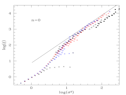
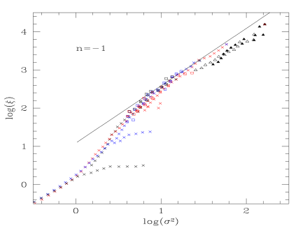
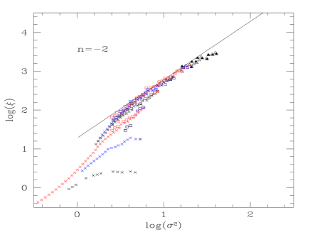
Since the initial conditions of the simulation are scale-invariant ( is a power-law) all curves should superpose as long as numerical effects (finite box size, softening length and resolution scale) are small. We can check that this is indeed the case. Moreover, in the highly non-linear regime we recover the asymptotic behaviour given by (12) which is shown by the solid line. The normalization parameter is displayed in Tab.1 for the three power-spectra. However, we can note that for larger scales the two-point correlation function “saturates” to a value lower than its asymptotic limit. This problem increases for smaller and is due to numerical effects since as we explained above all curves should superpose. The dependence on scale and on of this effect shows that it is produced by the lack of power in the simulation at large scales. Indeed, the actual initial power-spectrum is a power-law only over a limited range of and the influence of the numerical cutoff at , unduely supressing some power, becomes more important as one considers larger scales (hence wavenumbers closer to ) and lower (which increases the contribution of small ). Similarly, there is a high frequency cut-off. The correlation function starts to deviate from the exact scaling imposed by our power-law initial conditions when the sampling of the numerical output is done at the Mpc comoving scale and below. This is very distinctly seen in Fig.1 for the larger values of the correlation function. This is due to the softening of the interaction, which for all the samples we use is done over a radius of Mpc (comoving). Again, the result is a lack of power, due to this softening. Obviously, the deficit is larger for than for , the former case, with more small-scale power, being more sensitive to this effect.
Note that the Nyquist frequency and particle discreteness play a minor role if any at all since we only consider the cases where the number of points in the simulation is large enough.
3.2.2 Counts of neighbours
Although the average defined by (4) appears naturally when one considers counts in cells many authors studied the quantity given by:
| (13) |
which is relevant for the counts of neighbours. Indeed, the mean number of neighbours located within a radius from a given particle is:
| (14) |
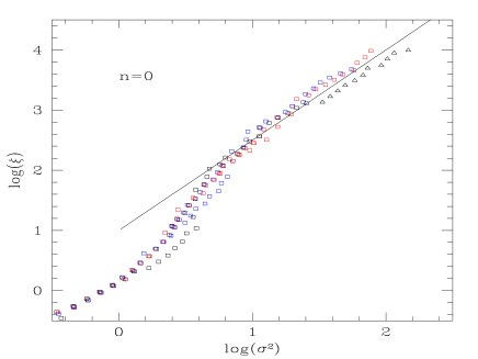
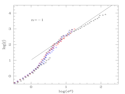
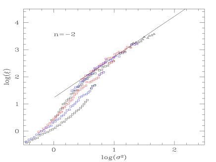
For a power-law power-spectrum depends on its linear equivalent in a fashion similar to (11) with a new function which has the same asymptotic behaviour as (12) but with a slightly different normalization (Hamilton et al.1991; Peebles 1980; see also Padmanabhan 1996). We measure in the simulation using (14): we count the mean number of neighbours of particles in the box which gives while the total number of points in the simulation provides . The result is shown in Fig.2. We indeed recover the behaviour predicted by (12). This confirms the previous results of Fig.1 since both and are measures of . This shows that in the non-linear regime the stable-clustering ansatz holds for which obeys the scaling-law (2).
Moreover, the measure of allows us to get a second estimate of in the non-linear regime. Indeed, in the domain where the two-point correlation function is a power-law with a slope given by (3) as shown by Fig.1 and Fig.2. In this case, one can show (Peebles 1980) that:
| (15) |
Thus, we can obtain from the measure of . These values are shown by squares in Fig.1. We can check that they agree with the previous calculations for based on the counts in cells. Note that we only show in Fig.1 the values of obtained from , through (15), which are in the highly non-linear regime where the two-point correlation function is a power-law so that (15) applies. Note that in this case (compare Fig.1 with Fig.2), the lack of power at the larger scales is much less pronounced: the count of neighbours already focuses on the dense regions and the statistics of the poorly represented events at large scale is improved. Indeed, to measure one considers cells which are centered on particles, hence this statistical tool follows the evolution of gravitational clustering as it automatically probes more closely denser regions, while to get the center of the cells is set at random in the box, so that in the highly non-linear regime most cells are within voids. Thus at least part of the deviations seen at these scales are due to the statistical extraction of the information.
We present in Tab.1 the values of the normalization parameters and obtained from our simulation, as well as from Jain et al.(1995) and Colombi et al.(1996). For the former we calculate from their value of while for the latter we obtain from . Indeed, from (15) we get:
| (16) |
where (resp. ) is given by (15) with (resp. ), corresponding to the non-linear (resp. linear) regime. Although all numerical simulations agree with the stable-clustering ansatz: (3), (11) and (12), the normalization of in the non-linear regime varies up to a factor 2 (note that it scales as the cube of ). Thus, there is still some inaccuracy in the numerical values of . Moreover, one may expect the higher-order correlation functions (hence the parameters ) to bear at least similar uncertainties. The discrepancies between the various estimates of may be due to the effects of finite volume and particle number: in particular the initial power-spectrum is not a power-law over an infinite range of scales (there are an upper and a lower cutoff) and one should average over many realizations of the initial gaussian field. However, the fact that curves obtained from different scales superpose in Fig.1 and Fig.2 and that our measures of are consistent with show that we can reasonably rely on our results. Except in the extreme cases where the finiteness of the sample (at large scales) or the smoothing of the force (at small scales) become important, these results are consistent with the idea that the stable clustering regime is reached (see however Padmanabhan et al.1996 for an alternative view).
3.2.3 Analytical fit to the fluctuations in a cell
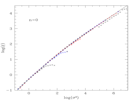
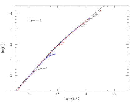
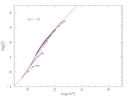
We show in Fig.3 the relation . This corresponds to an Eulerian point of view as opposed to the Lagrangian point of view displayed in Fig.1, since we now consider the values of the linear and non-linear correlation functions taken at the same spatial scale (and not at the same “mass scale”). We can note that the curves we obtain are quite smooth when displayed in this diagram and they do not show a sharp “step-profile” as was the case in Fig.1 and Fig.2. The solid lines are analytical fits to the numerical results which we shall need below (Sect.4) to get the mass functions within the framework of the scaling approach. Thus we use the approximations:
| (17) |
where . Of course, these fits are built so as to be consistent with (11) and (12). These relations define implicitly the functions . They will be used instead of the correlation function actually measured in the simulation (hence they will not be a source of unwanted deviations from self-similarity) when we determine the scaling properties of the multiplicity functions (Sect.4).
3.3 Counts in cells statistics
By counting the number of particles enclosed in each of spheres set on a grid, as we did to evaluate , we can also obtain the statistics of the counts in cells. This allows us to compare the predictions (5) of the scaling model to our numerical results for . Note that we obtain simultaneously the value of in the simulation, at the scale of interest, which we use in (5). We display the results in Fig.4 as a function of : from and obtained by these counts in the simulation we define:
| (18) |
If the scaling-laws (2) hold the quantity used above must be the scaling function defined in (5). Then, all curves obtained for different sizes and times should superpose. Note that in our case where the initial power-spectrum is a power-law all curves characterized by the same (or equivalently by the same ) must coincide. Thus the scaling-laws (2) merely imply in addition that curves measured for different should also superpose, when shown in a diagram as defined by (18).
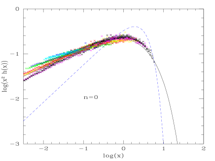
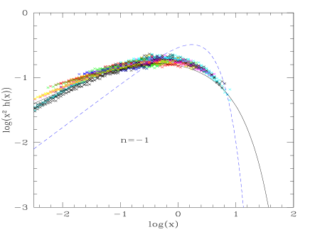
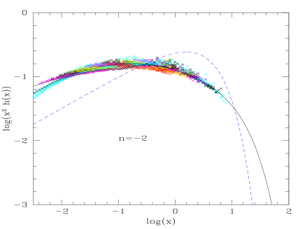
We can see in Fig.4 that the various curves indeed superpose, for all three power-spectra. Note that in this figure we only show the parts of which should scale as predicted by (5): we only display points which satisfy the requirements and . The solid curves are analytical fits to the data points. We use the functional form introduced by Bouchet et al.(1991):
| (19) |
The values of the parameters and are given in Tab.2. Note that the functions must also obey the constraints:
| (20) |
from the general relation (8).
The dashed curve in the figures is the function which one obtains (see VS) by assuming that the non-linear evolution of initial density fluctuations is given by the Press-Schechter approximation in the case where the correlation function has reached the stable clustering regime (which is indeed the case in the examples we have considered in Fig.4). Thus, we obtain what we shall refer to as the “PSs” estimate (“s” for stable)
| (21) |
the result being multiplied by the standard “PS factor” of two. For the stable clustering regime, , this expression is identical to the usual Press-Schechter formula (normally used for , the usual density contrast of just-virialized halos). If the above condition on is not fulfilled, only minor differences between the two expressions appear however, see Fig.7 below. We can see in Fig.4 that the function obtained in this way does not agree with the numerical results, the true distribution being much broader as argued by VS (the general trend, however, larger and sharper cutoff for higher is correct). This means either that one cannot follow the evolution of individual matter elements with using only the spherical model, because there is some exchange of matter between neighbouring density fluctuations through mergers and disruptions and the corrections to the spherical dynamics are not negligible, or that after virialization the density fluctuations still undergo non-negligible evolution. The stable-clustering ansatz on the other hand is seen from Fig.1 and Fig.4 to be a valid approximation in a statistical sense.
| 0 | 1.50 | 0.45 | 4 | 1 | 0.6 |
| -1 | 1.48 | 0.4 | 8 | 3 | 0.6 |
| -2 | 1.71 | 0.3 | 13 | 5 | 0.6 |
The scaling of the count-in-cells has thus been checked over an unprecedented range (more than 3 decades in the scaling parameter ). Note that we check here not only the scaling of the counts as a function of the cell size but also as a function of time, that is the self-similarity -in principle exact- of the computation results.
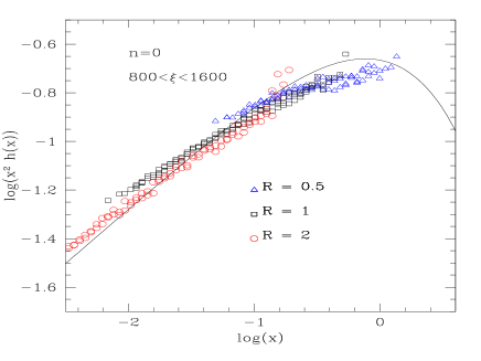
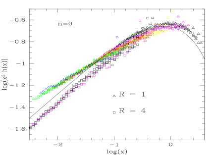
Although all curves at different scales superpose, building indeed the predicted universal curve, some deviations are seen for small values of the parameter . Clearly, these small values of ( !), never reached in earlier simulations, are at the limit of the possibilities of the present calculations, but the deviations appear to be systematic. For larger the function appears to be slightly flatter although it still obeys the constraints (20). Whether this effect is the sign of a real deviation of from the predicted scaling, or is due to some bias in the simulation, warrants investigation. To this purpose, we can consider the same simulation results in more detail. In the continuous limit (), the expression that in general depends on the three variables , the cell size and the expansion parameter , can always be written as , the latter expression representing a simple change of the original variables into , and . The exact self-similarity due to our power-law initial conditions implies that , as well as , are a function of the ratio only (i.e. they only depend on ) and thus that is independent of since carries all the dependence on and . The scaling prediction (due to the stable-clustering model) in addition states that in the limit of large , when the stable clustering regime is reached, has a limit for fixed that is independent of . By definition of this limit is . The scatter seen in Fig.4 must have its origin in the violation of one of the two above conditions that are needed to get the seeked scaling function. As a first check, we can consider the variations with at fixed . The value of the latter ranging from 100 to 6400, typical intermediate values are . In this range, values of and Mpc are available. We can see in Fig.5 (upper panel) that for these given values of , although the curves look reasonably close, there is a distinct drift at small , the curves for the smaller values of lying systematically above the ones for the lower values. Also, the deviations get larger the smaller the value of . Since we let vary for a fixed this effect represents deviations from the “exact” self-similarity (implied by scale-invariant initial conditions) due to the unavoidable errors in the simulation. To estimate the size of these deviations, we show in Fig.5 (lower panel) the probability distribution obtained for all possible values of keeping fixed at two values (1 and 4 Mpc). For a given , when is varied all curves superpose. But when is changed, we get a different curve. This shows again that depends on and not on , with a deviation that reaches a factor of 2 at small (), of the order of magnitude of the scatter seen in Fig.4. So we can attribute the observed scatter to deviations from the “exact”self-similarity (due to a power-law initial power-spectrum), hence to numerical inaccuracies and not to a violation of the non-linear scaling prediction that we aim to test here.
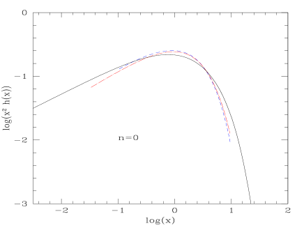
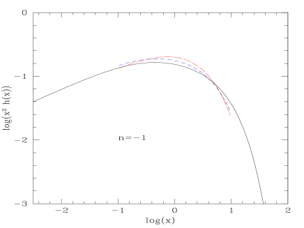
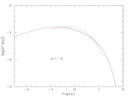
We compare in Fig.6 the scaling functions we get in our simulations with the results obtained by Colombi et al.(1997) and Munshi et al.(1999). For these two latter cases we only display over the ranges where there were actually data points from the simulations (for our scaling function the range tested against numerical results can be directly seen from Fig.4). We can check in the figure that all of the scaling functions agree fairly well with each other (within the numerical uncertainties which can be estimated from the dispersion shown in Fig.4). Thus, although there is still some dispersion between the various estimates of , which could be expected from the discrepancies which already appeared for , the scaling function is rather well constrained in the range where it has actually been tested, to an accuracy which is certainly sufficient for practical purposes. However, it should be noted that the range in available to constrain is still too small to determine accurately the parameters of the fit (19) for low , especially (there is some degeneracy between the exponential cutoff and the exponent of the power-law pre-factor). Thus, in the case the values of obtained by Colombi et al.(1997) and Munshi et al.(1999) differ by a factor 2, although both scaling functions are rather close over the range shown in Fig.6. This means that the asymptotic behaviour of , and more generally its behaviour for , typically, is still rather poorly determined.
3.4 Moments of the counts in cells
If one believes that the scaling function provides a reasonably good description of the counts-in-cells, it is readily seen from Fig.4 that the measured counts in the simulation miss the very rare overdensities at . In this region, actually there are counts that oscillate, due to (Bouchet et al.1992; Colombi et al.1995) whatever last cluster appears to be in the numerical data, reflecting their “cosmic variance”. It turns out that the calculation of the moments (4) badly reflects this missing information. The moments directly obtained from the measured counts are systematically underestimated, the effect being more pronounced as the scale of the cells increases. The moments depend most on the counts-in-cells at , as can be seen from (8) and (9). With and the calculation of , already, cannot be done without an extrapolation of the numerical data to the badly needed, but not measured large (large ) tail. Appropriate methods have been proposed by the above authors , but the resulting values of extracted from the data strongly reflect the precise extrapolation procedure used by the various authors (Colombi et al.1996; Munshi et al.1999) 111 To increase the available range, Colombi et al (1996) correct for the oscillations (typically a factor of 3 from the mean, sometimes an order of magnitude) due to this “cosmic variance” by means of an an educated guess, fitting a smooth curve of pre-determined shape to the data. To estimate the uncertainty, these authors determine by human judgement what can be considered as a reasonable fit and what cannot. This generates error bars given in the form of a factor (i.e. is within the range to ) with typically for , respectively, whereas the deviations from scaling show, under the same conditions, a scale-dependence by a factor , respectively. Their interpretation is that, since is typically larger than by , this “ prooves a small but significant departure from the stable clustering predictions” in the form of a scale-dependence of the coefficients . Whereas we think that such a procedure (see Colombi et al.1994) to extract information on the large behaviour, although somewhat indirect, is reasonable in the absence of any better way, it is not free from systematic biases and the associated correction may not be achieved at the accuracy needed to back the claim of the former authors. Indeed, a subsequent work (Munshi et al.1999), using a different computation, shows that the numerical data for large are at least consistent with the assumption of no scale-dependence at all of the coefficients . . The differences get rapidly very large with increasing order , from factors of 2 for to already an order of magnitude for . Thus extreme care must be taken in the interpretation of the parameters extracted from the simulations. Rather than introducing sophisticated corrections to extract the large tail of the counts (with uncontrolled errors due to the badly needed correction for cosmic variance) it may be as accurate (inaccurate) to simply fit a function to the numerical data and use (8) to get the moments.
4 Mass functions
For astrophysical applications, one is usually more interested in the mass functions (the number density of objects defined for instance by a given density threshold) than in the counts in cells statistics. Moreover, one may wish to study a wide variety of objects, from low-density Lyman- clouds (which may even be underdense!) to clusters and massive very dense galaxies (see for instance Valageas & Schaeffer 1999 and Valageas et al.1999 for a detailed description of Lyman- clouds and galaxies in this framework). Of course, these very different objects are defined by specific constraints so that they cannot be described solely by the mass function of “just-collapsed” halos with the traditional overdensity .
We have determined numerically the multiplicity of various kinds of idealized objects and compared them to theoretical predictions. To this purpose, we use two different methods. The fist is the “spherical overdensity” algorithm (Lacey & Cole 1994) which ranks particles in order of decreasing density and counts halos defined by the density contrast by looking down this list (this introduces some double counting since part of a halo may be counted again at a lower rank: to avoid this, when a new halo is recognized its particles are removed from the list). The second method is based on a friend-of-friend algorithm with a linking length which we relate to through:
| (22) |
4.1 The Press-Schechter approximation for just-collapsed halos
Most studies have focused on the mass function of “just-collapsed” (or “just-virialized”) halos which are defined by a density contrast in the actual non-linear density field (for ). Indeed, this is the quantity which is considered by the popular Press-Schechter prescription (Press & Schechter 1974). The idea of this formulation is to recognize in the early universe, when density fluctuations are still gaussian and described by the linear theory, which overdensities will eventually collapse and form virialized objects. Thus, one associates to any linear density contrast obtained by the linear theory ( for a given fluctuation of fixed mass) a non-linear density contrast provided by the spherical model. Next one assumes in addition that collapsed objects virialize at a radius equal for instance to one half their turn-around radius at the time when the spherical dynamics predicts a singularity. Then one obtains that when reaches the threshold a virialized halo with a density contrast has formed. Finally, one identifies the mass fraction within such objects of mass larger than with the fraction of matter which is above the threshold at scale in the linear universe:
| (23) |
Then, the mass-derivative of the previous quantity provides the mass function of virialized halos:
| (24) |
with
| (25) |
Here we defined as the fraction of matter which is enclosed in objects of mass to . Note that in (24) we have arbitrarily multiplied the mass function by the usual factor 2 so as to get the proper normalization to unity. We must however emphasize that this normalization correction is not justified in the present case. Indeed, although this multiplicative factor 2 was recovered rigorously by Bond et al.(1991) using the excursion sets formalism for a top-hat in , taking into account the cloud-in-cloud problem, this result does not apply to more realistic filters like the top-hat in used here. In fact, as shown in VS (and noticed by Peacock & Heavens 1990 through numerical results) this correction factor goes to unity at large masses. So, this factor is not constant (and equal to 2) but -dependent. This simple normalization procedure (24), nevertheless, leads to a scaling-law in the parameter : the mass function does not depend any longer on the initial power-spectrum. We present in Fig.7 the comparison of our numerical results with the PS prescription. We can check in the figure that the mass functions obtained by both methods are consistent. Note that the numerical points correspond to averages over different output times (weighted by the number of halos) of the mass functions realized in the simulations. Although there is some scatter we checked that all curves superpose on the mean mass function shown in Fig.7. We can note that our results are consistent with the scaling in obtained from the PS approach.
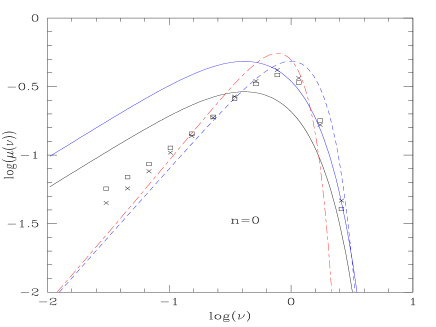
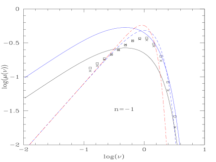
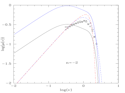
Thus, we can see as was already checked by many authors (e.g. Efstathiou et al.1988; Kauffmann & White 1993; Lacey & Cole 1994) that the Press-Schechter mass function (shown by the dashed line) agrees reasonably well with the numerical results. Indeed, although there are some small but significant discrepancies (especially at the low mass end where the slope seems to tend towards the non-linear prediction). This could be expected in view of the simplicity of this approach but the agreement is still rather good for such a simple model. A drawback of the Press-Schechter approach is that it is clearly limited to the mass function of “just-collapsed” objects and does not provide by itself predictions for mass functions defined at other density contrasts.
4.2 The scaling model for the halo multiplicity
Predictions for the mass function of objects defined by an arbitrary density contrast in the actual non-linear density field can be obtained within the framework of the scaling model, as shown in detail by VS. These predictions are valid for any value of , whatever large or small (even below unity!), provided the conditions (6) are met. As was the case for the counts in cells the mass function exhibits a scaling-law in the parameter :
| (26) |
where we still have . Note that here is the actual size of the halo (as opposed to the “mass scale” , the radius an object of the same mass would have in a uniform density universe, which enters for instance in the PS mass function). The scaling function should be related to introduced for the counts in cells. Indeed, if one identifies the mass within objects (defined by the density threshold ) larger than (i.e. more massive than ) with the fraction of matter enclosed in cells of scale with a density contrast larger than , one obtains a simple estimate of which reads
| (27) |
Even if this is probably an oversimplified approach, it has been steadily argued (Balian and Schaeffer 1989a ; Bernardeau and Schaeffer 1991; VS) at an increasing level of sophistication that the functions and can be expected to be close and that for practical purposes can be used as a good approximation to . Also, as can be seen in VS, this procedure is found to be very close to the global derivative used in the PS prescription (24). In the scaling model, however, it is applied to the actual non-linear density field rather than to the original Gaussian field, and thus is correctly normalised.
On the other hand, if one defines directly objects of scale to by the constraints that the density contrast is larger than on scale but smaller than on scale (thus one tries to recognize individually each halo in order to handle the cloud-in-cloud problem) one gets a new scaling function which can be shown (VS) to satisfy (for constant ):
| (28) |
with generically (unless the leading order in the expansion accidentally vanishes) the same asymptotic behaviour at small :
| (29) |
Moreover, for a tree-model where the many-body correlation functions can be expressed as products of the two-point correlation function one obtains for . Note that for a gaussian random field the same procedure (that is to define the mass function by requiring a given overdensity in the linear regime at a given scale and a lower one at a slightly larger scale, in order to recognize individually each object), would lead to a mass function which diverges at small masses (see VS), meaning divergent total mass due to the severe overcounting. Even for a fixed density contrast , the same mass is counted many times at smaller and smaller scales because of numerous density inversions. Since the fraction of matter (compared to unity) enclosed in objects defined by a density threshold is a direct measure of the severity of the “cloud-in-cloud” problem, this shows the latter is indeed severe for Gaussian fluctuations. On the other hand, in the non-linear case when one directly counts the overdensities in the non-linear density field, the normalization is necessarily lower than for the case described above from (28) and can be expected to be close to unity. This shows, as argued by VS, that in the non-linear regime, the overdensities being well-defined, there is no longer any serious cloud-in-cloud problem. The latter still manifests itself in the sense that the use of induces some slight overcounting, typically of the order of (see VS). This is the same overcounting as the one found in computations for the spherical density algorithm (which has been removed in this case by attributing all the mass to the larger object), and indeed of similar magnitude, as we checked in the numerical simulations. The true constraint, rather than the one on the edge of the halos used to define , which avoids this overcounting, is the condition that the density contrast is smaller than for all scales larger than . This would completely solve the cloud-in-cloud problem. However, the previous formulation leading to should already provide a satisfactory tool. Moreover, it is close to the algorithm actually used in numerical simulations.
The solid curves in Fig.7 represent the functions and . From the results described above, we expect the mass function obtained from the numerical simulations to lie below the upper curve for all and between these two curves for large (which corresponds to large ) beyond the exponential cutoff. We can see that this is indeed approximately the case for all power-spectra. However, it appears that the numerical mass function is significantly different from , especially at the low mass end. This could be expected since it does not seem possible to derive a lower bound for in this domain in the general case. Nevertheless, the slopes of both scaling functions appear to be the same for . Note that for large and () the mass function should not behave as (26) since this domain corresponds to large scales which are no longer in the non-linear regime, so the correlations functions do not obey the scaling (2). The dot-dashed lines correspond to the “PSs” mass function (26) given by the scaling approach with taken equal to the “spherical model” scaling function (21). Of course at small scales it superposes onto the standard PS mass function, as explained in Sect.3.3, since in this regime it is equivalent to the PS prediction. At large scales it differs from the latter because one leaves the highly non-linear, stable-clustering, regime and the two-point correlation function is no longer given by the asymptotic behaviour , see (12). Note that the PS approach works somewhat better for the mass function than it did for the counts in cells statistics, and that, for the contrast relevant to the present calculations, at large masses the difference with respect to the stable clustering PSs result somewhat helps. What helps also to bring the PS result in agreement with the numerical data is the factor of by which this mass function has been multiplied, as is traditional, despite numerical calculations (Peacock & Heavens 1990) as well as theoretical considerations (VS) show this factor should be close to unity at large (and is expected to be larger at small ).
As compared to the standard PS approach, the interest of the formulation (26) for the mass function of “just-virialized” objects is that it makes a connection with another characteristics of the density field: the counts in cells statistics described earlier.
4.3 Different constant density contrasts
The main advantage advantage of the scaling model is that it can deal with more general mass functions. We shall first consider the case of mass functions which are still defined by a constant density contrast but where can now take any value. In the scaling approach which led to (26) the quantity is only used to define objects but no specific value is singled out as opposed to the PS mass function which explicitly deals with “just-collapsed” objects (so that it makes sense for only one class of halos characterized by a non-linear density contrast ). Hence the relation (26) should hold for any value of , in the domain where the scaling (5) holds.
4.3.1 Spherical overdensity agorithm
We show in Fig.8 the mass functions we obtain from the numerical simulation for various values of the density contrast for the “spherical overdensity” algorithm. We display the quantity as a function of (as explained previously was obtained from the same simulation through counts in cells, see Fig.3). If the scaling (26) holds all curves should superpose (in the relevant range of validity of the scaling laws) onto the function (we only show the range which corresponds to but the range of validity could be smaller than this: ). The points correspond again to an average over different output times.
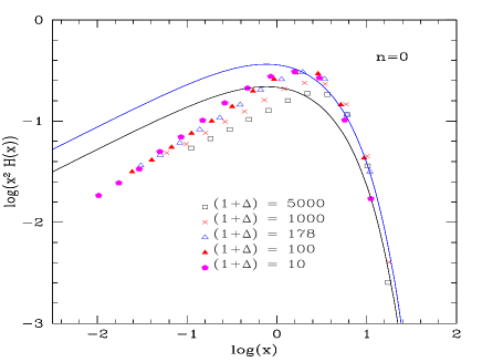
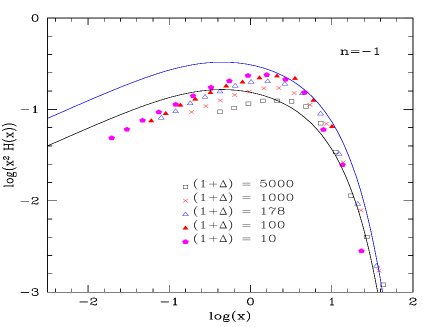
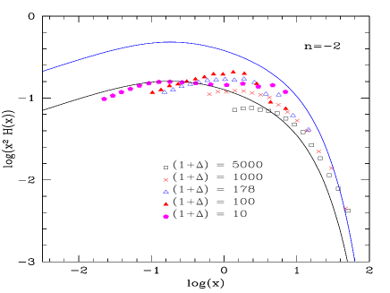
We can see that the available counts are pushed much further towards the larger values of as compared to Fig.4. This is because we check the neighbourhood of particles to get the halos and thus we are guaranteed to be in a region where there really is some mass. To get the statistics of the counts-in-cells, on the other hand, implies to check randomly over the whole volume, so that the statistics of the less dense but more extended regions are relatively favoured. As will be discussed in more detail in Sect.4.4, this amounts in some sense to measure rather than , with a better statistics at the large values of (note, however, that whereas has a maximum, both the above functions are decreasing for increasing , still favoring the small values of as compared to the large ones). A similar effect was described in Sect.3.2 for the measure of as opposed to .
As expected, all curves lie between and beyond the exponential cutoff and are located below for all values of . Moreover, the slope at small is in most cases close to that for , although for , where the statistics are the best, a distinct difference is apparent: whereas has a slope (Tab. 2) , here the slope is rather .
Moreover, although all curves superpose beyond the cutoff as predicted, there appears to be a shift in the power-law domain with : larger density contrasts lead to a smaller amplitude in this part of the mass function. This drift appears at for and for and has disappeared for (indeed the curves obtained for superpose very well).
These deviations will be discussed in the following section.
4.3.2 Friend-of-friend algorithm
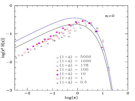
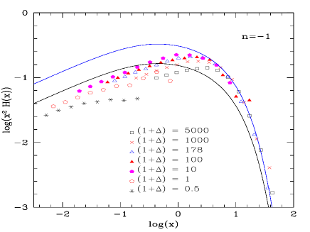
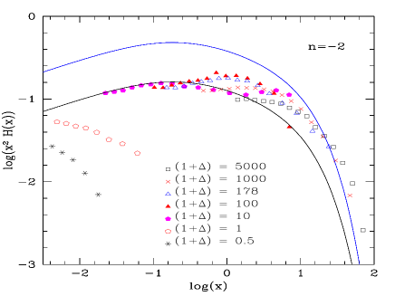
We show in Fig.9 the mass functions we obtain from the “friend-of-friend” algorithm. We can check that they are consistent with the results from the “spherical overdensity” algorithm. For large we find as previously that the curves superpose beyond the exponential cutoff but that there is a drift in the power-law domain.
The advantage of the “friends-of-friends” algorithm is that we can also consider negative density contrasts, providing for much larger a range for the possible variations of . In such a case we count one large halo which extends over the whole box (the clusters linked by the filaments create a percolating network) and also small underdense objects which appear as density peaks within voids and are separated from the main cluster by their very low density surroundings. Thus, the mass function defined in this way only makes sense for very small masses (small parameter ). Despite the low density, this is still in the strongly non-linear regime since so that .
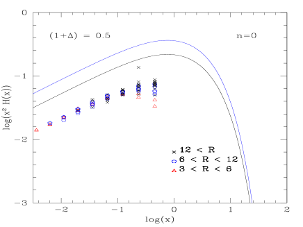
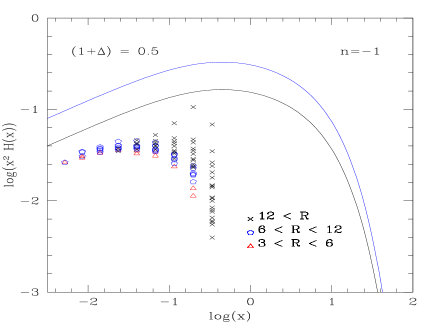
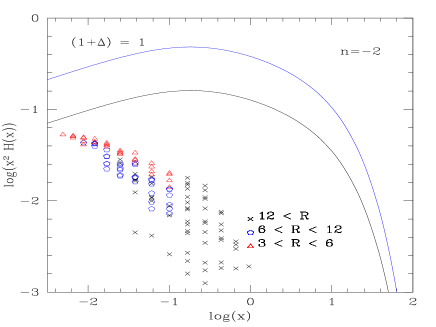
For , we can see that all curves fall on top of each other, down to which is a little low at . Similarly, for , the results exhibit the scaling theoretically implied by the stable clustering, except for at the larger values of (). For , also, the curves with and do not fall on the scaling curve built by the result at larger density contrasts. As shown in Fig.10, the deviations found for the lower values are seen to be closely associated to the degradation of the statistics (the counts are low at the larger ), that occurs for all three values of we have studied precisely at the same values of and where the deviations are noticed. Moreover, the deviation at large of the mass functions measured for low density contrasts () from the scaling predictions corresponds to the fact that they only make sense for small since we must have so as to avoid entering the linear regime where there are no dense spots within underdense regions like the ones we look for here.
So, the non-linear scaling prediction is seen to hold down to values of that are unity or even smaller. This is nearly three orders of magnitude below the standard density contrast of usually studied. It has also been tested down to , a real improvement as compared to existing work: values below had never been considered previously.
Note that the slopes at small of the mass function are close to the ones predicted by the theory. In the case, for instance, , quite close to the slope of . The offset seen in Fig.8 with the “spherical overdensity” algorithm does not exist in this case. It should be noted that the case with clearly shows (Fig.9) that the non-linear power-law prediction (and perhaps more important, the prediction of existence !) for objects that are much denser than their close environment is well verified even in this quite extreme case of very low density, definitely below the average.
Towards the higher densities, we have run calculations up to , a factor of above the usual densities. As for the spherical density algorithm, scaling is well verified. Similarly, at the smaller values of , steadily increasing deviations appear when is increased, although to a lesser extent. For and , the curve for is below the one for (that at fixed corresponds to correlation functions times smaller, hence to scales times larger at fixed time) by a factor 1.35 and below the curve by a factor 1.7. The relevant scales are the smallest reachable in the simulation, typically Mpc at and Mpc at , for . This is to be compared with the force softening parameter which is Mpc in all the calculations presented here. We have checked the sensitivity of the calculations to variations of this softening parameter. Decreasing the latter by a factor of so as to increase the effect of collisions, lowers the counts by a factor of at the scales considered above (a change quite comparable to the deviations from scaling that were found), but has no effect at the larger values of (the larger scales). For the calculation of the correlation function, at , similarly, deviations of the computation appeared at small scales. So, there is a limit towards the large densities and the smaller values of beyond which the numerical tests are no longer conclusive, since binary collisions due to the discreteness of the points in the simulation start to play a non-negligible role.
Although the previous discussion leads to attribute the lack of objects below some value of , for a given (large) density contrast, to the fact that the smallest available scale in the simulation has been reached, this is an important point to be discussed. Note that the theoretical prediction (see VS) for extends to all values of (including the lower ones for which there are no numerical data) and that, whatever the density contrast, the area under the scaling curve is unity (it is actually slightly above for , but is unity if corrections to avoid double counting are made). This means that however large the required density threshold is, it defines a way to distribute all the mass among objects having this density contrast. The theoretical prediction thus calls for very strong subclustering at all density levels. On the other hand, the simulations do not provide enough power at small for large overdensities: there is barely more than of the mass in objects of contrast 5000, for instance, showing an increasing lack of high density objects. Again, this apparent difference is worth to be thoroughly investigated in future more extended simulations, to see whether subclustering up to extremely high overdensities is present down to very small scales or not. However, as shown in Valageas (1999), note that the reasonable agreement of the numerical results with our scaling model already shows that there is a large amount of subclustering. It has been steadily argued (Balian & Schaeffer 1989a,b) that the existence and the behaviour of these substructures are the base of the scaling model and govern the properties of the density field.
We have tested the scaling model for the multiplicity function for vastly different density contrasts, spanning four orders of magnitude, from to , finding non-linear objects at every density. We have shown that up to the small-scale limit where collision effects begin to play a role and to the low-density limit where deviations from self-similarity start to appear the scaling model provides a reasonable approximation to the mass functions obtained in the simulations. Also, we can note that the scaling model gives surprisingly good results in domains which are beyond its expected range of validity. For instance, the curves for and agree in the numerical results down to . Hence, although the model may not be perfect it is still quite powerful as it allows one to get a good estimate of the mass functions of very different objects. Moreover, it clarifies an interesting link with another statistical analysis of the density field, namely the counts in cells.
4.4 Constant radius
In practice, one may also be interested in objects which are no longer defined by a constant density threshold but by a condition of the form . The predictions of the scaling model for such a case were studied in VS. It happens that for astrophysical objects like galaxies or Lyman- clouds the constraints which define these mass condensations can be approximated in some range by the requirement that their radius is constant and equal to a given scale which may be associated in the first case to a cooling radius and in the second to a Jeans length (see Valageas & Schaeffer 1999 and Valageas et al.1999 for more details). This corresponds to the limit . Then, one has to add the supplementary constraint that the density profile is locally decreasing (since one usually wants to consider peaks and not valleys). In this specific case one obtains the relations (see VS):
| (30) |
for the simple model. More realistically, one can define (see VS) a scaling function for the mass distribution of objects of fixed radius and make the statistics of the overdensity -hence of the mass since we have - by requiring for such a halo to have a density contrast larger than at scale and smaller than at a slightly larger scale. Thus one considers individually each object, defined by the fixed radius and its density contrast (which gives its mass), making sure that it is surrounded by regions of lower density. Then, one obtains the bounds
| (31) |
Obviously this procedure is quite similar to the counts in cells so we can expect the scaling function to be very close to .
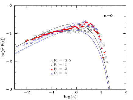
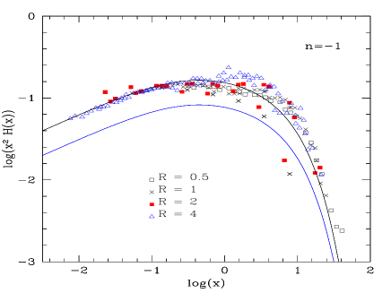
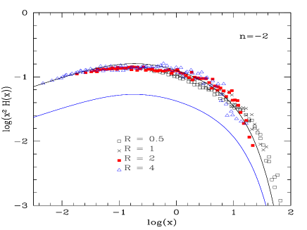
We show in Fig.11 the mass functions obtained in this way from the numerical simulations. We simply use a modified version of the “spherical overdensity algorithm”, looking at particles in order of decreasing density and defining halos as objects of constant size around density peaks. The scaling with the variable is well verified, for all values of the spectral index , with a result that is very close to the prediction (30). There seems, nevertheless, to be more counts at large (large masses): the first of the bounds (31) of the “improved” estimate (in the sense it is closer to the spherical overdensity procedure) seems to be somewhat violated. Note however that the curves obtained for different radii (and times) superpose fairly well which shows the predicted scaling in is verified (within the numerical scatter). In fact, this small deviation is probably due to the definition of itself and not to a failure of the scaling-laws (2). Indeed, this estimate of the mass function is derived from specific counts-in-cells (with the characteristic that these cells consist of an internal sphere surrounded by a small corona) so that one can miss the most massive high density halos by looking at a sphere which is not exactly centered onto the underlying halo. This decreases the mass enclosed in this sphere, which is maximum for a cell correctly centered. On the other hand, in the simulation one directly draws the spheres from the highest density peaks, so that one always counts the largest amount of matter which can be attached to a given halo (if the object is approximately spherically symmetric). This latter procedure (looking at the peaks) is not included in and, because of this small “mis-placement” of the spheres, it slightly underestimates the number of very high density and massive halos. We note that a similar, but very small, deviation may be seen for the mass functions shown in Fig.8 and Fig.9, for the same reason. We also note that the mass function shown in Fig.11 allows one to probe deeper into the exponential cutoff of , hence of , as compared to the counts in cells shown in Fig.4. This could also be expected from the fact that in this procedure “cells” are drawn directly around highest density peaks, which are thus well accounted for, while for the statistics of density peaks can be divided between several cells.
5 Conclusion
In this article we have presented a comparison of the results obtained from numerical simulations to the analytical predictions implied by the Press-Schechter (Press & Schechter 1974) prescription and the scaling model (Balian & Schaeffer 1989a ; VS).
We have first checked that the two-point correlation functions follow the behaviour predicted by the stable-clustering ansatz, as shown by other studies. However, although there is a qualitative agreement between various works the exact value of the amplitude of the two-point correlation function in the highly non-linear regime still remains poorly determined as there remains some discrepancy between different studies. Next we have shown that the scaling model provides a good description of the counts in cells statistics. The characteristic scaling functions we obtain over the unprecedented range agree reasonably well with previous estimates. Nevertheless, the asymptotic behaviour of the exponential cutoff is not very well constrained for due to the limited range of scales available in the simulations.
Then we considered the mass function of “just-collapsed” objects, which is the quantity most authors have focussed on. As was already noticed by many studies, we find that the PS approximation works reasonably well for density contrasts of (although there are some discrepancies). On the other hand, the numerical results are also consistent with the predictions of the scaling model (although they do not provide the exact value of the mass function). Next we have studied more general mass functions defined by various density contrasts that vary by four orders of magnitude (including negative density thresholds!). The scaling model (which is the only currently available analytical tool to handle these quantities) was shown to provide a reasonable estimate of these mass functions.
Finally, we considered the limiting case of objects defined by a constant radius constraint (which arises in an astrophysical context from cooling conditions). We have shown that the scaling model also works very well for such mass functions. Some small deviations appear in certain regimes. We make specific suggestions on which biases may appear in the simulations and show they are of the right order of magnitude. Although these biases likely explain the observed scatter, it is quite clear that we cannot check the scaling prediction better than this scatter. It remains to be verified in more powerful simulations whether (at least part of) these deviations can be attributed to some violation of the scaling predicted by theory, or if these deviations indeed disappear and thus simply reflect the fact that we have pushed the present simulation as far as possible, and reached its limits.
Thus, the scaling model provides a reasonable description of the density field in the non-linear regime (although there are some deviations in certain regimes they remain reasonably small for practical purposes). Moreover, it allows one to link two different properties of the latter: the counts in cells statistics and the mass functions. In addition, it can be used to obtain many different mass functions (in addition to the usual “just-collapsed”halos) which is of great interest for practical purposes when one intends to model various objects like Lyman- clouds or galaxies which clearly cannot be defined by the sole constraint . Obviously, our study should be extended to more realistic power-spectra which are no longer power-laws (e.g. CDM) and to different cosmologies (low-density universes).
References
- [1]
- [2] Balian R., Schaeffer R., 1989a , A&A 220, 1
- [3] Balian R., Schaeffer R., 1989b , A&A 226, 373
- [4] Bernardeau F., Schaeffer R., 1991, A&A 250, 23
- [5] Bernardeau F., 1996, “Large-scale structure formation”, XXXIth Moriond meeting, Les Arcs, France, Ansari R., Giraud-Heraud Y., Tran T hanh Van J., eds. Frontieres, p. 187
- [6] Bond J.R., Cole S., Efstathiou G., Kaiser N., 1991, ApJ 379, 440
- [7] Bouchet F.R., Schaeffer R., Davis M., 1991, ApJ 383, 19
- [8] Colombi S., Bouchet F.R., Schaeffer R., 1994, A&A 281, 301
- [9] Colombi S., Bouchet F.R., Schaeffer R., 1995, ApJS 96, 104
- [10] Colombi S., Bouchet F.R., Hernquist L., 1996, ApJ 465, 14
- [11] Colombi S., Bernardeau F., Bouchet F.R., Hernquist L., 1997, MNRAS 287, 241
- [12] Couchman, H.M.P., 1991, ApJ 368, 23
- [13] Davis M., Peebles P.J.E., 1977, ApJS 34, 425
- [14] Davis M., Efstathiou G., Frenk C., White S.D.M., 1985, ApJ 292, 371
- [15] Efstathiou G., Frenk C.S., White S.D.M., Davis M., 1988, MNRAS 235, 715
- [16] Hamilton A.J.S., Kumar P., Lu E., Matthews A., 1991, ApJ 374, L1
- [17] Jain B., Mo H.J., White S.D.M., 1995, MNRAS 276, L25
- [18] Kauffmann G., White S.D.M., 1993, MNRAS 261, 921
- [19] Lacey C., Cole S., 1994, MNRAS 271, 676
- [20] Munshi D., Bernardeau F., Melott A.L., Schaeffer R., 1999, MNRAS 303, 433
- [21] Padmanabhan T., 1996, MNRAS 278, L29
- [22] Padmanabhan T., Cen R., Ostriker J.P., Summers F.J., 1996, ApJ 166, 470
- [23] Peacock J.A., Heavens A.F., 1990, MNRAS 243, 133
- [24] Peebles P.J.E., 1980, The large scale structure of the universe, Princeton University Press
- [25] Peebles P.J.E., 1982, ApJ 263, L1
- [26] Press W., Schechter P., 1974, ApJ 187, 425
- [27] Valageas P., 1999, A&A 347, 757
- [28] Valageas P., Schaeffer R., 1997, A&A 328, 435 (VS)
- [29] Valageas P., Schaeffer R., 1999, A&A 345, 329
- [30] Valageas P., Schaeffer R., Silk J., 1999, A&A 345, 691
- [31] Valageas P., Silk J., 1999, A&A 347, 1