For submission to Monthly Notices
Self-consistent Gravitational Lens Reconstruction
Abstract
We present a new method for directly determining accurate, self-consistent cluster lens mass and shear maps in the strong lensing regime from the magnification bias of background galaxies. The method relies upon pixellisation of the surface mass density distribution which allows us to write down a simple, solvable set of equations. We also show how pixellisation can be applied to methods of mass determination from measurements of shear and present a simplified method of application. The method is demonstrated with cluster models and applied to magnification data from the lensing cluster Abell 1689.
keywords:
Cosmology: theory – large–scale structure of the Universe, gravitational lensing; Galaxies: clusters1 Introduction
The possibility of reconstructing cluster lens mass distributions from the magnification bias of background galaxies was first suggested by Broadhurst, Taylor & Peacock (1995) and first demonstrated by Taylor et al. (1998, T98 hereafter). They showed how a direct, local measure of the lens convergence, , where is the mass surface density and is the critical surface density, could be obtained from knowledge of the lens magnification. In this way, one could measure absolute surface mass densities, thereby breaking the “sheet-mass” degeneracy found in methods based on distortions of background galaxies (Tyson, Valdes & Wenk 1990, Kaiser & Squires 1993, Seitz & Schneider 1995).
van Kampen (1998) and T98 have shown how one can extend magnification analysis into the strong lensing regime. By making reasonable assumptions about , the lens shear, they showed that one could place quite stringent bounds on . In addition, T98 found an exact solution for the profile of axisymmetric lenses, although not for more general 2D cases.
Inverse reconstruction methods based on maximum likelihood (Bartelmann et al. 1996) and maximum entropy (Seitz, Schneider & Bartelmann 1998, Bridle et al. 1998) have gone some way in providing a unification of both shear and magnification information. Until now however, no direct method using only magnification has existed.
In this letter, we show how to directly compute an accurate, self-consistent 2D distribution of and in the strong lensing regime from magnification. This direct approach has the advantage over indirect alternatives that uncertainties can easily be determined. The method is based on pixellisation of the distribution suggested by AbdelSalam, Saha & Williams (1998) who used it to estimate the mass of Abell 370 from multiple images. We generalise the method further and also derive a simplified solution to the problem of estimating mass from shear, based on the approach of Kaiser & Squires (1993).
2 Reconstruction of and
T98 showed how to estimate cluster surface mass using the magnification measured from the distortion in background galaxy number counts. Here our problem is to find an accurate method for reconstructing the surface mass density, given the magnification by an arbitrary lens. The inverse magnification factor at a given position in the lens plane is
| (1) |
where is the lens convergence and is the shear. The shear can be decomposed into two orthogonal polarisation states, and , which are related to the lens convergence by
| (2) |
where and is the 2D inverse Laplacian. The total shear is given by . One might expect that equation (1) could be solved iteratively by first estimating , using this to calculate and then updating the estimate of using equation (1) again. This proves to be highly unstable in the strong lensing regime however, rapidly diverging after only a few iterations (Seitz & Schneider 1995).
To find a stable solution to equation (1), we first pixellise the image. Following AbdelSalam et al. (1998), we can now write
| (3) |
with summation implied over index and where and are the pixellised convergence and shear distributions respectively. The transformation matrices, , are
| (4) | |||||
and
| (5) | |||||
with the integration acting over the pixel. is the difference between pixels and which are assumed to be square in calculating these analytic expressions. Equation (1) can now be written as the vector equation,
| (6) |
where is the -dimensional vector of pixellised inverse magnification values, is the transpose of the vector of pixellised convergence values and is the vector . The matrix is the matrix
| (7) |
where is the Krönecker delta, and summation is only over indices and . The parity of the measured inverse amplification is handled by which flips from being outside regions bounded by critical lines to within such regions.
3 Application to Cluster Models
We apply the method to two types of idealised cluster models. Starting with a predetermined cluster mass density distribution, the corresponding shear distribution is derived using Fourier methods (see for example, Bartelmann & Weiss 1994). From these, the resulting magnification is calculated from equation (1) and then windowed to remove boundary effects. Using equation (6), we solve for . is then solved using equation(3). A grid of 32 by 32 pixels is used in both models.
3.1 Truncated Isothermal Sphere Model
We first test the method with a simple truncated isothermal lens model. The pixellated mass distribution is laid down using , where is the radial distance from the centre of the sphere and is a constant.
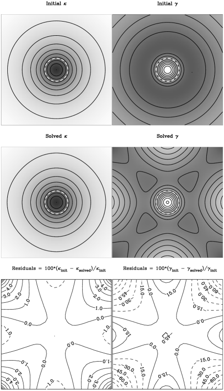
Figure 1 shows the and distribution from which the magnification distribution was calculated, the solved and distribution and the difference between them. The plotted distributions are smoothed from the underlying grid and the white dashes highlight the lens’ critical line. The residuals are shown as percentage deviations from the true distribution. These are less than one percent for over most of the grid which is negligible in comparison to the errors typically found in practice from background clustering, shot noise (T98) and the uncertainties resulting from use of local estimators (see van Kampen 1998). The recovered shear distribution is more affected although still fares better than calculated from uncorrected Fourier techniques. The main contribution to these residuals is from boundary effects arising from trying to recover a nonlocal shear in a finite area. Since much work has been carried out into the removal of such effects (see Squires & Kaiser 1996 and Seitz & Schneider 1995 for example) which have little impact on the recovered , we shall address the problem elsewhere.

3.2 Dumb-bell Mass Model
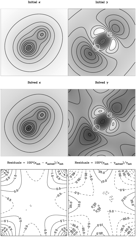
The method was also tested with a more general dumb-bell model. Magnification was determined in the same fashion as for the isothermal model, setting a negative parity inside the critical lines, shown by the white dashes in figure 2. Once again the residuals between the initial and solved are typically less than one percent, while those for are typically and again come mainly from boundary effects.

4 Practical Considerations
We solve equation (6) with the hybrid Powell method (NAG routine C05PCF). The number of equations needed to solve for is equal to the total number of grid pixels which can prove computationally intensive for especially fine grids. We find that this is not a problem for grid resolutions used to measure magnification bias in practice however. The 32 by 32 grid of pixels used for the models in section 3 was solved in approximately one minute on an average workstation. The residuals exhibit no noticeable dependence on grid size.
The Powell algorithm is an iterative process and therefore requires an initial estimate of the solution to start from. The choice of the initial estimate turns out to be irrelevant. We have tried a wide range of initial distributions and even starting from a uniform distribution arrived at the same final solution.
We have found that correct choice of pixel parity (especially for low grid resolutions) is essential in order to achieve a sensible result. Inappropriate assignment of parities to pixels manifest themselves, as one would expect, by being overestimated when a pixel is wrongly assumed to lie inside a critical line and underestimated in the reverse situation. This gives a means of checking whether critical line positions have been properly defined by looking for large discontinuities in the distribution. Models with dual critical lines requiring dual parity flips have also been tested and we find that can be recovered just as well.
Finally, to ensure that the method does not break down with noisy data, we introduced a random noise term to the amplification. Errors in resulting from noise in the inverse amplification propagate as one would expect from equation (6). For an isothermal lens we recovered the expected result, , indicating that pixellisation does not lead to spurious noise properties.
5 Application to Abell 1689
We apply the method to the magnification data presented in T98 for the lensing cluster A1689. A 12 by 12 grid is used as the best compromise between shot noise in galaxy counts per bin and the resolution of the derived map. Identification of the critical line was achieved by locating giant arc positions in the observed image.
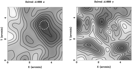
Figure 3 shows the solved mass density and shear distribution. Comparison with the mass density map illustrated in T98 (figure 6) which was produced with the sheet estimator shows very similar structure. We find that the value of at the peak calculated here is approximately 10% lower than the peak value in T98 since the sheet estimator over-estimates inside critical line regions. This has little effect on the total integrated mass of A1689 found in T98. The distribution is shown for completeness although undoubtedly suffers from boundary effects typically found in the models.

6 Shear Analysis
Having shown that pixellisation allows us to accurately reconstruct surface mass densities from magnification data, we now apply it to shear analysis. Shear analysis exploits the idea that a given distribution of images of galaxies lying behind a lensing cluster will, in the statistical mean, have regions of lens-induced correlations in image orientation and ellipticity. Measuring the quadrupole moments of individual galaxy images enables the construction of a map of the ellipticity parameters, (Valdes, Tyson & Jarvis 1983). The ellipticity parameters relate to the surface mass density and shear via (Kaiser 1995, K95 hereafter):
| (8) |
One way of solving this for in the weak lensing regime is to follow the approach of Kaiser & Squires (1993). Generalisations of this to the strong regime have been made by K95. One would have hoped that an alternative to such approaches would be to pixellise equation (8) and use equation (3) to solve it by matrix inversion. However, the resulting matrix equation is ill-conditioned, since the matrix is singular and is itself ill-conditioned. Instead, we show a new, simplified expression for the solution to Kaisers’ ellipticity equation and then pixellise it.
Starting with the equation (K95),
| (9) |
and using equation (8), one can show that
| (10) |
The term on the right hand side is obtained from the definition,
| (11) |
where is the identity matrix and is an arbitrary square matrix. Using this expansion and collecting even and odd terms we find,
| (12) |
where and . This result requires that . Inserting equation (8) into the magnification equation (1) we find
| (13) |
Hence the parity changes when . Since and are observationally indistinguishable and flip from one to another whenever there is a parity change, we can satisfy the criterion just by noting the critical line positions and inverting the ellipticity matrix when one is crossed.
Finally, inserting equation (12) into equation (10), and solving for we find the pixellised solution is
| (14) |
where
| (15) |
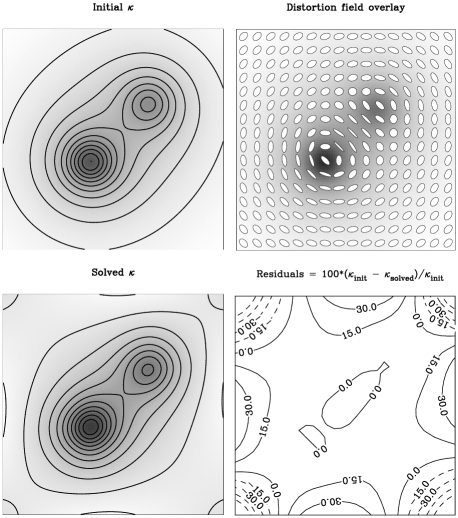
Equation (14) is the second main result of this letter. We can directly calculate given a measured ellipticity field. Figure 4 shows the results of reconstructing using equation (14) for the dumb-bell model. The ellipticity parameters are calculated from equation (8) using the and distribution. We normalise the reconstructed to both peaks in the initial distribution. The residuals, again being dominated by boundary effects, show that reconstruction is possible to within approximately 10 percent across the field of view.

7 Summary
We have outlined a method for directly calculating accurate, self-consistent surface mass density and shear distributions from the lens amplification and critical line positions. The method has been demonstrated with the isothermal sphere and dumb-bell cluster models. We find it reconstructs the surface density to within a percent over most of the field of view. The reconstruction of the shear pattern only has fractional accuracy of a few tenths due to boundary effects. We have applied the method to magnification data from Abell 1689, and reconstructed its surface mass and shear distribution.
We have also found a simplified solution to the problem of estimating surface mass density from galaxy ellipticities. This approach puts the calculation of surface mass from shear and magnification on an equal footing, and we shall investigate the combined analysis elsewhere.
ACKNOWLEDGEMENTS
SD is supported by a PPARC studentship. ANT is a PPARC research associate. Thanks to our collaborators Tom Broadhurst, Txitxo Benitez, Eelco van Kampen for allowing us to use data from Abell 1689. We also thank Hanadi AbdelSalam for bringing the benefits of pixellisation to our attention and for useful discussion.
REFERENCES
AbdelSalam H.M., Saha P., Williams L.L.R., 1998, MNRAS, 294, 734
Bartelmann M., Narayan R., Seitz S., Schneider P., 1996, ApJ, 464, 115
Bartelmann M., Weiss A., 1994, A&A, 287, 1
Bridle S.L., Hobson M.P., Lasenby A.N., Saunders R., 1998, astro-ph/9802159
Broadhurst T.J., Taylor A.N., Peacock J.A., 1995, ApJ, 438, 49
Kaiser N., (K95), 1995, ApJ, 439, L1
Kaiser N., Squires G., 1993, ApJ, 404, 441
Seitz C., Schneider P., 1995, A&A, 297, 287
Seitz C., Schneider P., Bartelmann M., 1998, astro-ph/9803038
Squires G., Kaiser N., 1996, ApJ, 473, 85
Taylor A.N., Dye S., Broadhurst T.J., Benitez N., van Kampen E., (T98), 1998, ApJ, 501, 539
Tyson J.A., Valdes F., Wenk R.A., 1990, ApJ, 349, L1
Valdes F., Tyson J., Jarvis J., 1983, ApJ, 271, 431
van Kampen, 1998, submitted to MNRAS