DATA COMPRESSION FOR CMB EXPERIMENTS
Abstract
We discuss data compression for CMB experiments. Although “radical compression” to bands, via quadratic estimators or local bandpowers, potentially offers a great savings in computation time, they do a considerably worse job at recovering the full likelihood than the the signal-to-noise eigenmode method of compression.
We model a CMB observation at a pixel , as , where and represent the contribution of the CMB signal and the noise, respectively, to the observation. The signal is given by ; is the spherical harmonic decomposition of the temperature and encodes the beam and any chopping strategy of the experiment.
We also assume that both the signal and noise contributions are described by independent, zero-mean, gaussian probability distributions, with correlation matrices given by and , so here, is calculated as a function of , the parameters of the theory being tested in the likelihood function, and the noise matrix can include the effect of constraints due to, e.g., average or gradient removal. For Gaussian theories of adiabatic fluctuations, is typically the cosmological parameters; alternately they could be some set of phenomological parameters such as the value of the temperature power spectrum in some bands.
With this notation, the likelihood function is
| (1) |
Calculating this requires extensive manipulations on the total correlation matrix over extensive portions of the parameter space. Herein lies the problem: in order to calculate the determinant factor in the denominator requires time of .
We can state the problem as follows: find some functions of the data, such that the new likelihood, and is “easier to calculate” in some appropriate sense. The definition of “” in this expression is crucial. If we take it to mean “having the same variance,” the requirement reduces to the definition of “lossless” involving the Fisher matrix.[1] Note that this requirement will only be adequate very near the maximum of the distribution, i.e., where the Gaussian approximation is appropriate. For large data-sets, with high signal-to-noise, this will presumably be an adequate description; elsewhere (including those parts in the “tails” of an otherwise high-S/N experiment’s window function that may be most interesting), it will not necessarily obtain that the derived confidence limits and parameter estimates will be the same.
If we can find a basis in which the matrices and are diagonal, the likelihood computation simplifies from matrix manipulations to sums and products. First, we whiten the noise matrix using the transformation provided by its “Hermitian square root,” and apply the same transformation to , diagonalizing this in turn with the appropriate matrix of eigenvectors, , in units of . We then transform the data into the same basis, , in units of . In this basis, the noise and signal have diagonal correlations and . Now, the likelihood function is a simple product of one-dimensional uncorrelated gaussians in .[2]
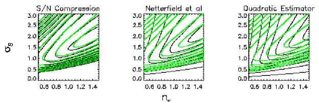
Modes with low are linear combinations of the data which probe the theory poorly. Thus, they are ideal candidates for removal in a data compression scheme. Removal of these low-S/N modes is the optimal way to compress the data: for a given number of modes, it removes the most noise and least signal. Of course, the modes will change as the shape of the theory used for the covariance matrix changes. In that case, we choose some fiducial theory (here, standard, untilted CDM) that represents the data moderately well, calculate its S/N-eigenmodes, and choose some number of modes to retain after compression. For other theories, these modes will not be optimal—we will have removed more signal and less noise. Nonetheless, this method does quite well even far from the fiducial theory, as we see in the Figure, which shows the likelihood for a parameterization of a standard CDM power spectrum with amplitude, , and a scalar tilt, (so the primordial ). Unfortunately, finding this basis is ; even performing this operation once for a megapixel dataset will be prohibitively expensive.

Most experiments report their results in the form ; this encourages the use of a simple curve-fitting approach to parameter estimation[3]: form the obvious quantity where is the predicted power spectrum for the theoretical parameters . In practice, the power spectrum is usually reported as a flat bandpower over some band with an appropriate window function, but the procedure remains the same.
Now, just do the usual fast -minimization for the parameters. This is a very “radical” approximation to the full likelihood: it assigns an uncorrelated gaussian distribution to the power spectrum: . In the figure, we show confidence intervals for the SK95 experiment with the full likelihood and compare them to those obtained with 1) the S/N compression discussed above; 2) using flat bandpowers as reported by Netterfield et al;[4]; 3) using a quadratic estimator of in bands of , modified somewhat to minimize covariance[5]. The peaks are nearby, and the contours are similar in the “amplitude” direction (), but less good in the “shape” () direction. Far from the peak, all of the methods do quite poorly. The location of the peak is determined by the gross shape of the power spectrum, so the details of the calculation do not matter; this is especially true when combining the results of experiments probing very different scales, such as COBE/DMR and SK95. Away from the peak, the shape of the spectrum within the experimental windows, the covariances of the errors, and the non-Gaussian shape all contribute to the determination of which theories are more highly disfavored.
References
References
- [1] M. Tegmark, astro-ph/9611174, Ap. J., submitted, 1996.
- [2] J.R. Bond & A. Jaffe, Phys. Rev. Lett., submitted, 1997; A. Jaffe & J.R. Bond, in preparation, 1997.
- [3] C. Lineweaver, these proceedings.
- [4] C.B. Netterfield, M.J. Devlin, N. Jarosik, L. Page, & E.J. Wollack, Ap. J. 474, 47 (1997).
- [5] L. Knox, J.R. Bond & A. Jaffe, these proceedings; M. Tegmark & A. Hamilton, these proceedings.