Relativistic Hydrodynamic Flows Using Spatial and Temporal Adaptive Structured Mesh Refinement
Abstract
Astrophysical relativistic flow problems require high resolution three-dimensional numerical simulations. In this paper, we describe a new parallel three-dimensional code for simulations of special relativistic hydrodynamics (SRHD) using both spatially and temporally structured adaptive mesh refinement (AMR). We used the method of lines to discretize the SRHD equations spatially and a total variation diminishing (TVD) Runge-Kutta scheme for time integration. For spatial reconstruction, we have implemented piecewise linear method (PLM), piecewise parabolic method (PPM), third order convex essentially non-oscillatory (CENO) and third and fifth order weighted essentially non-oscillatory (WENO) schemes. Flux is computed using either direct flux reconstruction or approximate Riemann solvers including HLL, modified Marquina flux, local Lax-Friedrichs flux formulas and HLLC. The AMR part of the code is built on top of the cosmological Eulerian AMR code enzo. We discuss the coupling of the AMR framework with the relativistic solvers. Via various test problems, we emphasize the importance of resolution studies in relativistic flow simulations because extremely high resolution is required especially when shear flows are present in the problem. We also present the results of two 3d simulations of astrophysical jets: AGN jets and GRB jets. Resolution study of those two cases further highlights the need of high resolutions to calculate accurately relativistic flow problems.
Subject headings:
hydrodynamics–methods:numerical–relativity1. Introduction
Relativistic flow problems are important in many astrophysical phenomena including gamma-ray burst (GRB), active galactic nuclei (AGN), as well as microquasar and pulsar wind nebulae, among others. Apparent superluminal motion is observed in many jets of extragalactic radio sources associated with AGN. According to the currently accepted standard model, this implies the jet flow velocities as large as of the speed of light (Blandford et al., 1977; Begelman et al., 1984). Similar phenomena are also seen in microquasars such as GRS 1915+105 (Mirabel & Rodriguez, 1994) and GRO J1655-40 (Tingay et al., 1995) thus by similar arguments relativistic flows are thought to play a role. In the case of GRB, the observed non-thermal spectrum implies that the source must be optically thin, which can be used to put a limit on the minimum Lorentz factor within those bursts (Lithwick & Sari, 2001). This argument shows that the source of GRB must be in highly relativistic motion. This conclusion is further confirmed by the rapidly increasing number of GRB afterglow observations by the Swift satellite (Gehrels et al., 2004). To understand physical processes in those phenomena quantitatively, high resolution multi-dimensional simulations are crucial.
Jim Wilson and collaborators pioneered the numerical solution of relativistic hydrodynamics equations (Wilson, 1972; Centrella & Wilson, 1984; Hawley et al., 1984a, b). Starting with these earliest papers this has typically been done in the context of general relativistic problems such as accretion onto black holes and supernovae explosions. The problem was recognized to be difficult to solve when the Lorentz factor becomes large (Norman & Winkler, 1986) and a solution with an implicit adaptive scheme was demonstrated in one dimension. Unfortunately, this approach is not generalizable to multi-dimensions. However, in the past two decades accurate solvers based on Godunov’s scheme have been designed that have adopted shock-capturing schemes for Newtonian fluid to the relativistic fluid equations in conservation form (for a review see Martí & Müller, 2003). Such schemes, called high-resolution shock-capturing (HRSC) methods, have been proven to be very useful in capturing strong discontinuities with a few numerical zones without serious numerical oscillations. We will discuss a number of them in section 3.
Studies involving astrophysical fluid dynamics in general are benefiting tremendously from using spatial and temporal adaptive techniques. Smoothed particle hydrodynamics (Gingold & Monaghan, 1977; Lucy, 1977) is a classic example by being a Lagrangian method. Increasingly also variants of Berger & Colella (1989)’s structured adaptive mesh technique are being implemented. This is also true in relativistic hydrodynamics (Hughes et al., 2002; Anninos et al., 2005; Zhang & MacFadyen, 2006; Morsony et al., 2006; Meliani et al., 2007) where certainly the work of Hughes et al. (2002) showed that a serial AMR code could solve problems even highly efficient parallel fixed grid codes would have difficulty with. In this paper we discuss our implementation of different hydrodynamics solvers with various reconstruction schemes as well as different time integrators on top of the enzo framework previously developed for cosmology (Bryan & Norman, 1997a, b; Bryan et al., 2001; O’Shea et al., 2004). This new code we call renzo is adaptive in time and space and is a dynamically load balanced parallel using the standard message passing interface.
In the following we briefly summarize the equations being solved before we give details on the different solvers we have implemented. Section 4 discusses the adaptive mesh refinement strategy and implementation. We then move on to describe various test problems for relevant combinations of solvers, reconstruction schemes in one, two and three dimensions, with and without AMR. Section 6 presents an application of our code to three-dimensional relativistic and supersonic jet propagation problem. Section 7 discusses 3d GRB jet simulation. We summarize our main conclusions in section 8.
2. Equations of Special Relativistic Hydrodynamics
The basic equations of special relativistic hydrodynamics (SRHD) are conservation of rest mass and energy-momentum:
| (1) |
and
| (2) |
where is the rest mass density measured in the fluid frame, is the fluid four-velocity (assuming the speed of light ), is the Lorentz factor, is the coordinate three-velocity, is the energy-momentum tensor of the fluid and semicolon denotes covariant derivative.
For a perfect fluid the energy-momentum tensor is
| (3) |
where is the relativistic specific enthalpy, is the specific internal energy, is the pressure and is the spacetime metric.
SRHD equations can be written in the form of conservation laws
| (4) |
where the conserved variable is given by
| (5) |
and the fluxes are given by
| (6) |
Anile (1989) has shown that system (4) is hyperbolic for causal EOS, i.e., those satisfying where the local sound speed is defined as
| (7) |
The eigenvalues and left and right eigenvectors of the characteristic matrix , which are used in some of our numerical schemes, are given by Donat et al. (1998).
The conserved variables are related to the primitive variables by
| (8) | |||||
| (9) | |||||
| (10) |
where . The system (4) are closed by an equation of state (EOS) given by . For an ideal gas, the EOS is,
| (11) |
where is the adiabatic index.
3. Numerical Schemes for SRHD
3.1. Time Integration
We use method of lines to discretize the system (4) spatially,
| (13) | |||||
where refers to the discrete cell index in directions, respectively. , and are the fluxes at the cell interface.
As discussed by Shu & Osher (1988), if using a high order scheme to reconstruct flux spatially, one must also use the appropriate multi-level total variation diminishing (TVD) Runge-Kutta schemes to integrate the ODE system (13). Thus we implemented the second and third order TVD Runge-Kutta schemes coupled with AMR.
The second order TVD Runge-Kutta scheme reads,
| (14) | |||||
| (15) |
and the third order TVD Runge-Kutta scheme reads,
| (16) | |||||
| (17) | |||||
| (18) |
where is the final value after advancing one time step from .
For an explicit time integration scheme, the time step is constrained by the Courant-Friedrichs-Lewy (CFL) condition. The time step is determined as
| (19) |
where is a parameter called CFL number and is the local largest speed of propagation of characteristics in the direction whose explicit expression can be found in Donat et al. (1998).
3.2. Reconstruction Method
Generally speaking, there are two classes of spatially reconstruction schemes (see e.g. LeVeque 2002). One is reconstructing the unknown variables at the cell interfaces and then use exact or approximate Riemann solver to compute the fluxes. Another is direct flux reconstruction, in which we reconstruct the flux directly from fluxes at the cell centers. To explore the coupling of different schemes with AMR as well as exploring which method is most suitable for a specific astrophysical problem, we implement several different schemes in both classes.
To reconstruct unknown variables, we have implemented piecewise linear method (PLM, Van Leer 1979), piecewise parabolic method (PPM, Colella & Woodward 1984, Martí & Müller 1996), the third-order convex essentially non-oscillatory scheme (CENO, Liu & Osher 1998). These are used to reconstruct the primitive variables since reconstructing the conserved variables can produce unphysical values in SRHD. Furthermore, unphysical values of three-velocities may arise during the reconstruction especially for ultrarelativistic flows. So we either use to do the reconstruction or we also reconstruct the Lorentz factor and use it to renormalize the reconstructed three-velocity when they are unphysical.
For direct flux reconstruction, we have implemented PLM and the third and fifth order WENO scheme of Jiang & Shu (1996). Direct flux reconstruction using WENO was first used to solve SRHD problems by Zhang & MacFadyen (2006). They showed that the fifth order WENO scheme works well with the third order Runge-Kutta time integration. In our implementation, we followed their description closely. For the PLM and CENO schemes, we used a generalized minmod slope limiter (Kurganov & Tadmor, 2000). For given , , where . For it reduces to the monotonized central-difference limiter of Van Leer (1977). We found that this generalized minmod slope limiter behaves much better than a traditional minmod limiter (LeVeque, 2002) especially for strong shear flows. In our calculation, is used by default. For the PPM scheme, we used the parameters proposed by Martí & Müller (1996) for all the test problems. For WENO, we used the parameters suggested in the original paper of Jiang & Shu (1996).
3.3. Riemann Solvers
In the first class of reconstruction methods, given the reconstructed left and right primitive variables at interfaces, the flux across each interface is calculated by solving the Riemann problem defined by those two states. An exact Riemann solver is quite expensive in SRHD (Martí & Müller, 1994; Pons et al., 2000). Thus we have implemented several approximate Riemann solvers including HLL (Harten et al., 1983; Schneider et al., 1993; Kurganov et al., 2001), HLLC (Toro et al., 1994; Mignone & Bodo, 2005), local Lax-Friedrichs (LLF, Kurganov & Tadmor 2000) and the modified Marquina flux (Aloy et al., 1999).
The HLLC scheme is an extension of the HLL solver developed by Toro et al. (1994) for Newtonian flow which was extended to two-dimensional relativistic flows by Mignone & Bodo (2005). The improvement of HLLC over HLL is restoring the full wave structure by constructing the two approximate states inside the Riemann fan. The two states can be found by the Rankine-Hugoniot conditions between those two states and the reconstructed states. With this modification, HLLC indeed behaves better than other Riemann solvers in some 1d (§ 5.1.7) and 2d (§ 5.2) test problems. But when we apply HLLC to three dimensional jet simulation, we found that HLLC suffers from the so called “carbuncle” artifact well-known in the computational fluid dynamics literature (Quirk, 1994). We have used HLLC to run many other two-dimensional test problems designed to detect the carbuncle artifact and confirmed this shortcoming. We found that the HLLC solver is unsuitable for many multi-dimensional problems. The discussion of these problems will be presented elsewhere. In this work, we will only apply HLLC to two test problems showing that the HLLC solver has less smearing at contact discontinuities than other schemes.
Lucas-Serrano et al. (2004) has compared the HLL scheme, the LLF scheme and the modified Marquina flux formula using 1d and 2d test problems. They found those three schemes give similar results for all their test problems. In our tests, we found similar results. However, the modified Marquina flux formula is not as stable as HLL in problems with strong transverse flows and LLF is more diffusive than HLL. So in the following discussion we will only show the results using HLL in most of the tests if there is no difference among those three schemes.
In the following discussion, we will denote a specific hydro algorithm by X-Y where X is the flux formula and Y is the reconstruction scheme. For example, F-WENO5 denotes direct flux reconstruction using fifth order WENO. We used the third order Runge-Kutta method for all the tests in this work.
3.4. Converting Conserved Variables to Primitive Variables
Since primitive variables are needed in the reconstruction process, after every RK time step, we need to convert conserved variables to primitive variables. While conserved variables can be computed directly from primitive variables using Eqs. (8), (9) and (10), the inverse operation is not straightforward. One needs to solve a quartic equation for the ideal gas EOS and a nonlinear equation for more complicated EOS. Iteration methods are used even for ideal gas EOS, because computing the solution of a quartic is expensive. Following Aloy et al. (1999), we have used a Newton-Raphson (NR) iteration to solve a nonlinear equation for pressure to recover primitive variables from conserved variables. Typically, the NR iteration needs only to steps to converge.
3.5. Curvilinear coordinates
We have also implemented cylindrical and spherical coordinates following the description of Zhang & MacFadyen (2006). This affects three parts of the code. Firstly, the geometric factors are incorporated into the flux when updating the conserved variables. Secondly, there will be geometric source terms. Thirdly, the flux correction in AMR (§ 4.4) is modified by geometric factors.
4. Adaptive Mesh Refinement
4.1. Overview
Structured adaptive mesh refinement (AMR) was developed by Berger & Oliger (1984) and Berger & Colella (1989) to achieve high spatial and temporal resolution in regions where fixed grid resolution is insufficient. In structured AMR, a subgrid will be created in regions of its parent grid needing higher resolution. The hierarchy of grids is a tree structure. Each grid is evolved as a separate initial boundary value problem, while the whole grid hierarchy is evolved recursively.
renzo is built on top of the AMR framework of enzo (Bryan & Norman, 1997a; O’Shea et al., 2004). enzo’s implementation of AMR follows closely the Berger & Colella paper and has been shown to be very efficient for very high dynamic range cosmological simulations (see e.g. Abel et al. 2002). The pseudocode of the main loop for the second order Runge-Kutta method reads,
The RebuildHierarchy function called at the end of every time step is at the heart of AMR. Its pseudocode as implemented originally in enzo reads,
| (20) | |||
4.2. Interpolation
When a new subgrid is created, the initial values on that grid are obtained by interpolating spatially from its parent grid. In this case, we apply the conservative second order order interpolation routine provided by enzo to conserved variables. But in this process sometimes the interpolated values can violate the constraint . If this happens, we will then use first order method for that subgrid.
Before the first Runge-Kutta step for a grid at level (in the following discussion, we use the convention that top grid has level ), we will need the boundary condition at time , which is derived by interpolating from its parent grid. Then at the later steps of Runge-Kutta scheme, one needs the boundary condition at time . Since the variables of its parent grid has already been evolved to time , which is greater than time , we can obtain the boundary conditions at time for a grid at level by interpolating both temporally and spatially from its parent grid. There are two exceptions to this procedure. First, if a cell of fine grid abuts the box boundary, then we just use the specified boundary condition for that cell. Second, if a cell abuts another grid at the same level, we copy the value from that grid. Because of the above mentioned problem for interpolating conserved variables, when interpolating boundary values, we apply the second order interpolation to primitive variables. Since for ultrarelativistic flows spatially interpolating three-velocity can lead to unphysical values, we also interpolate the Lorentz factor and then use it to renormalize the interpolated three-velocity.
4.3. Refinement Criteria
In the test problems discussed in section 5, we mainly used two general purpose refinement criteria that have been widely used in AMR code (Zhang & MacFadyen, 2006).
In the first one, we compute the slope
| (21) |
where is typically density, pressure and velocities, is a small number typically taken to be . When is larger than a minimum slope, typically , a cell will be flagged for refinement.
In the second one, for every cell we compute
| (22) |
which is the ratio of the second and first derivatives with a safety factor in the denominator. Unless otherwise stated, we use . When is larger than a critical value , a cell will be flagged for refinement. Typically we use .
To fully exploit AMR, it is desirable to design more specific refinement criterions that are most efficient for a specific astrophysical problems.
4.4. Flux Correction
When a cell is overlayed by a finer level grid, then the coarse grid value is just the conservative average of the fine grid values. On the other hand, when a cell abuts a fine grid interface but is not itself covered by any fine grid, we will do flux correction for that cell, i.e. we will use the fine grid flux to replace the coarser grid flux in the interface abutting the fine grid.(see Berger & Colella 1989 for more detailed description of flux correction). For this purpose, note that the second order Runge-Kutta method can be rewritten as
| (23) |
and the third order Runge-Kutta method can be rewritten as
| (24) |
Thus for example, when we do flux correction in the -direction for interface , we will use and to correct the coarser grid conserved variables for the second and third order Runge-Kutta method, respectively.
4.5. Parallelism
renzo uses the enzo parallel framework which uses dynamically load balancing using the Message Passing Interface (MPI) library. At run time, the code will move grids among processors according to the current load of every processor to achieve a balanced distribution of computational load among processors. The computational load of a processor is defined as the total number of active cells on that processor and level.
5. Code Tests
5.1. One Dimensional Test
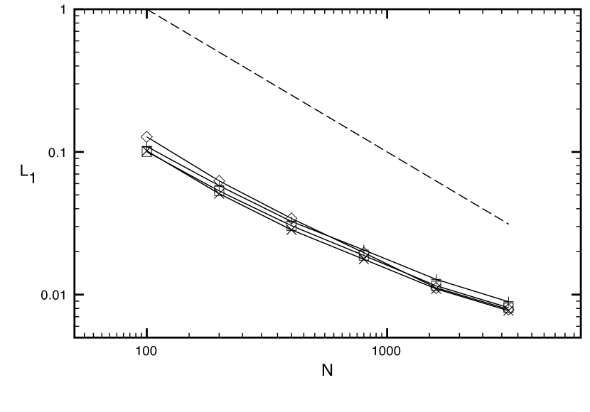
Relativistic Riemann problems have analytical solutions (Pons et al., 2000), thus they are ideal for tesing SRHD codes. In the following discussion, subscript and refer to the left and right initial states, respectively. The initial discontinuity is always at . We will report the error between numerical solutions and analytical solutions using norm defined as where is the numerical solution, is the analytical solution and is the cell width.
5.1.1 Relativistic Blast Wave I
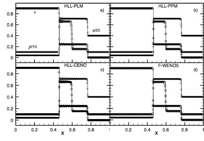
This test and the following one are fairly standard and all modern SRHD codes can match the analytical solution quite well (see Martt́ & Müller 2003 for a summary of different codes’ performance on those two tests).
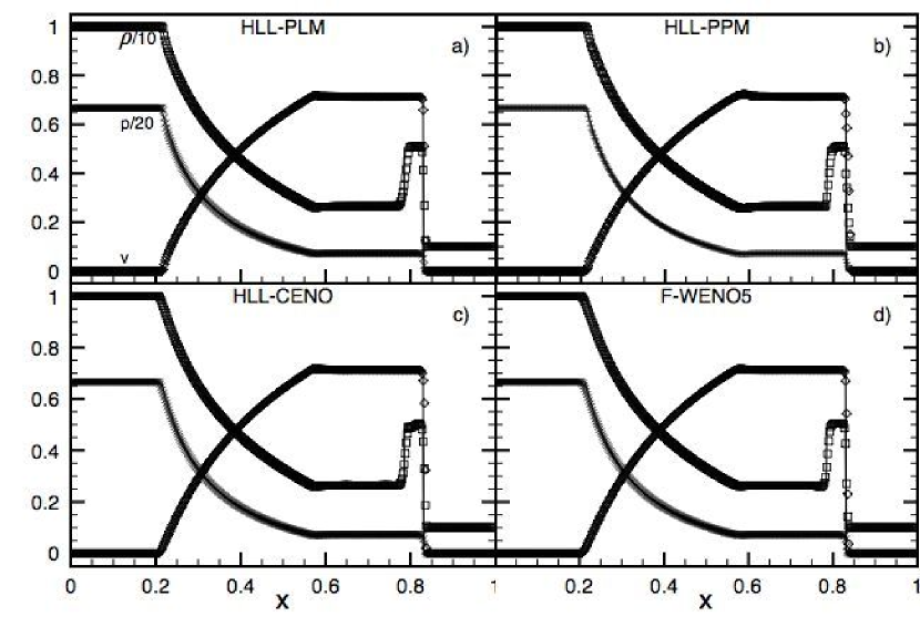
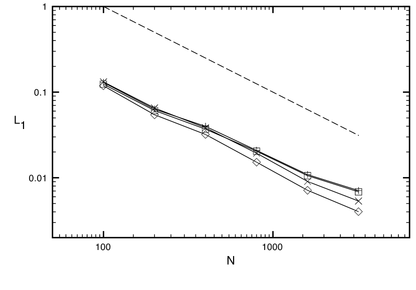
The initial left and right states for this problem are and , , . The gas is assumed to be ideal with an adiabatic index . The initial discontinuity gives rise to a transonic rarefaction wave propagating left, a shock wave propagating right and a contact discontinuity in between. This problem is only mildly relativistic with a post-shock velocity and shock velocity 0.83. The results using four hydro solvers are shown in Fig. 1. The CFL number used is . The errors are shown in Fig. 2, from which we can see the four schemes behave essentially identical for this problem. The order of global convergence rate is about 1 for all four schemes, which is consistent with the fact that there are discontinuities in the problem.
5.1.2 Relativistic Blast Wave II
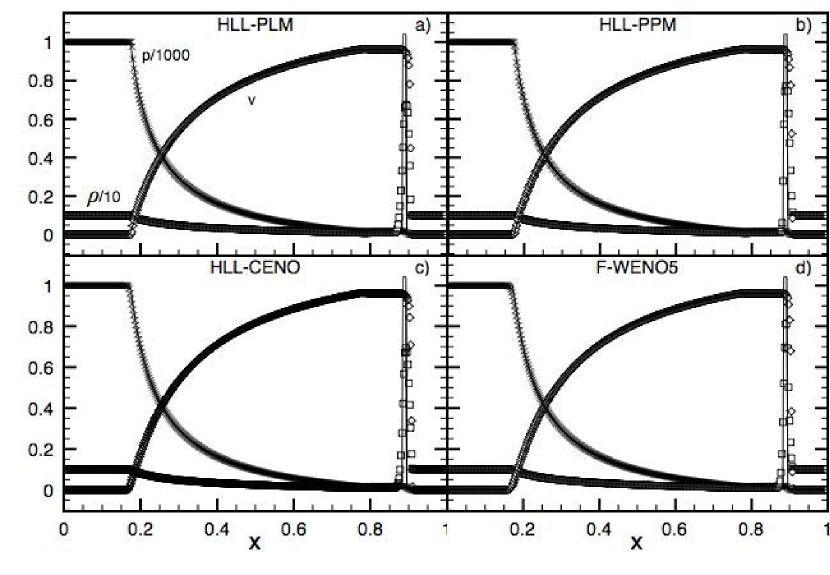
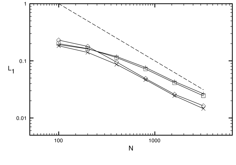
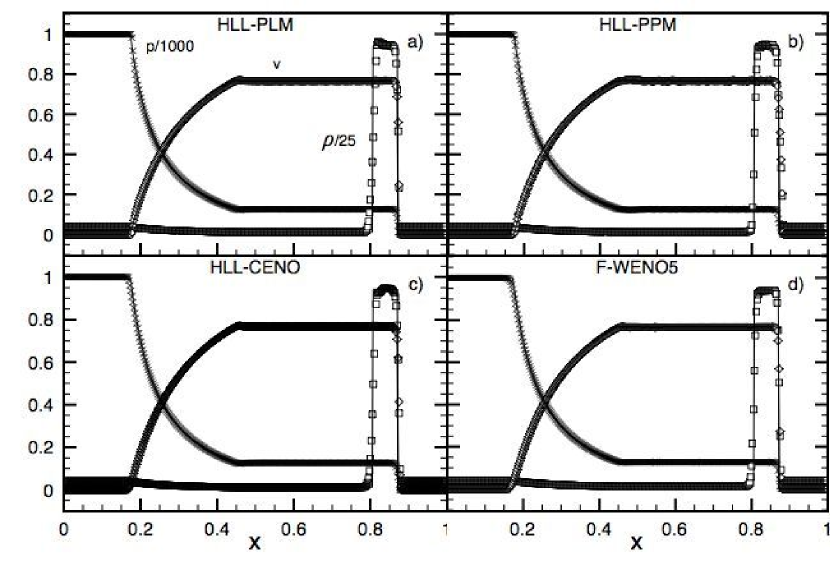
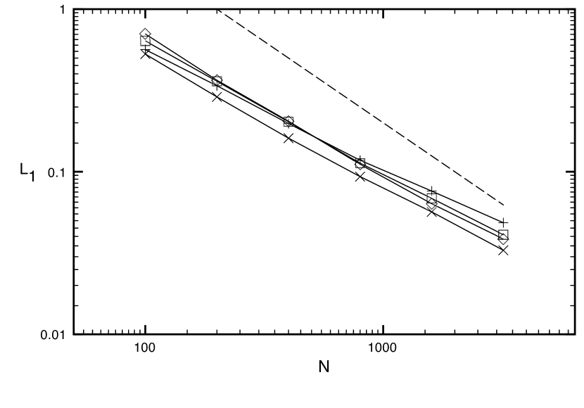
The initial left and right states for this problem are and , , . The gas is assumed to be ideal with an adiabatic index . This test is more relativistic than the previous one. While the wave structure is the same, the thermodynamically relativistic initial left state gives rise to a relativistic shock propagating at a Lorentz factor and a very thin dense shell behind the shock with width at . The CFL number used is . The results using four hydro algorithms are shown in Fig. 3. The errors are shown in Fig. 4. We can see that for this problem PPM and WENO have smaller errors than PLM and CENO. This is due to their ability to better resolve the thin shell.
5.1.3 Planar Jet Propagation
The initial left and right states for this test are and , , . The gas is assumed to be ideal with an adiabatic index . This test mimics the interaction of a planar jet head with the ambient medium. The decay of the initial discontinuity gives rise to a strong reverse shock propagating to the left, a forward shock propagating to the right and a contact discontinuity in between. The results are shown in Fig. 5. The CFL number is . The errors are shown in Fig. 6. As can be seen in Figs. 5 & 6, for this problem PPM and WENO behave better than PLM and CENO: there is almost no oscillation behind the reverse shock and they capture the contact discontinuity with fewer cells. Especially PPM captures the contact discontinuity with only cells and has the smallest error.
5.1.4 Blast Wave with Transverse Velocity I
For this and the following two problems, we will consider non-zero transverse velocities in the initial states. The initial state is identical to blast wave problem II except the presence of transverse velocities. Those problems were first discussed analytically by Pons et al. (2000). Since then various groups have shown that when transverse velocities are non-zero, in some cases those problems become very difficult to solve numerically unless very high spatial resolution is used (Mignone et al., 2005; Zhang & MacFadyen, 2006; Morsony et al., 2006). In realistic astrophysical phenomena transverse velocities are usually very important (see e.g. Aloy & Rezzolla 2006), thus solving those problems accurately is of great importance.
As an easy first case, we will consider non-zero transverse velocity only in the low pressure region. The initial left and right states are and . The gas is assumed to be ideal with an adiabatic index . The results are shown in Fig. 7. The CFL number is . The errors are shown in Fig. 8. We can see that all four hydro algorithms behaves similarly well, except that PLM and CENO shows some small oscillations around the contact discontinuity.

5.1.5 Blast Wave with Transverse Velocity II
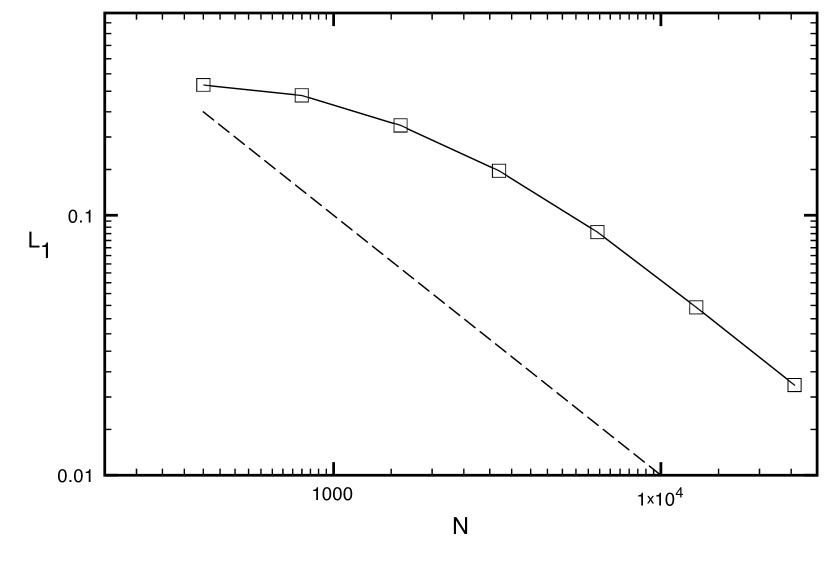
Next, we consider non-zero transverse velocity in the high pressure region. In this case, the problem becomes more difficult to solve numerically (Mignone et al., 2005; Zhang & MacFadyen, 2006). The initial left and right states for this problem are and . The gas is assumed to be ideal with an adiabatic index . The high pressure region is connected to the intermediate state by a rarefaction wave. Since the initial normal velocity in the high pressure region is zero, the slope of the adiabat increases rapidly with transverse velocity, thus a large initial transverse velocity will lead to a small intermediate pressure and a small mass flux.
The results using a uniform grid and two AMR runs are shown in Fig. 9. The hydro solver used for this figure is HLL-PLM. The CFL number is . The error are shown in Fig. 10. It can be seen that for the run with 400 uniform grid cells, the numerical solution is inadequate, as previously found by Mignone et al. (2005). This is mainly due to the poor capture of the contact discontinuity. We have tried to run this problem with various algorithms but only obtained accurate solutions by dramatically increasing the resolution.

| Equivalent Resolution | BT II | BT III |
|---|---|---|
| 400 | 400 | 400 |
| 800 | 448 | 421 |
| 1600 | 455 | 442 |
| 3200 | 470 | 468 |
| 6400 | 501 | 473 |
| 12800 | 518 | 476 |
| 25600 | 562 | 520 |
5.1.6 Blast Wave with Transverse Velocity III
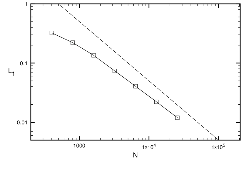
Now we introduce transverse velocity in both region. The initial left and right states for this problem are and . The gas is assumed to be ideal with an adiabatic index . This problem is more difficult than the previous one due to the formation of an extremely thin shell between the rarefaction wave tail and the contact discontinuity (Zhang & MacFadyen, 2006).
The results with a uniform grid and two AMR runs are shown in Fig. 11. The hydro solver used for this run is HLL-PLM. The CFL number used is . The errors are shown in Fig. 12.
Table 1 shows the equivalent resolution and the actual number of cells used for this and the previous tests. It can be seen for the highest resolution calculation our code uses about four hundred times less grid cells than the corresponding uniform grid calculation. Thus AMR allows us to achieve very high resolution while significantly reducing the computational cost.

5.1.7 Jet-Cocoon interaction
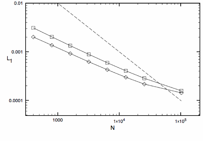
For this test we set up a one-dimensional Riemann problem that mimics the interaction of jet with an overpressured cocoon. The initial left and right states for this problem are and . The gas is assumed to be ideal with . Those values mimic the conditions of the jet-cocoon boundary in model C2 of Marti et al. (1997). The result using four different Riemann solver with PLM on uniform grid are shown in Fig. 13. It can be seen that solutions use HLL, LLF and direct flux reconstruction have large positive fluctuations in the normal velocity at the rarefaction wave. It is interesting to note that only HLLC does not suffer from this shortcoming which is probably due to the ability of HLLC to resolve the contact discontinuity compared to the other Riemann solvers in the code. If those fluctuations also happen in higher dimensional jet simulation, then one would expect that the normal velocity fluctuation seen in this test would lead to an artificially extended cocoon.
In Fig. 14 the result of using HLL-PLM and HLLC-PLM with AMR is shown. It can been seen that the fluctuation in the HLL scheme becomes smaller with higher resolution. Fig. 15 shows the error for those two schemes with different levels of refinement.

5.2. Two Dimensional Test: Shock Tube
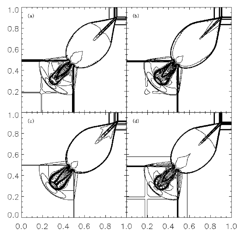
To test the code in higher dimension, we first study the two-dimensional shock tube problem suggested by Del Zanna & Bucciantini (2002) and latter also used by various groups (see e.g. Zhang & MacFadyen 2006, Mignone & Bodo 2005a, Lucas-Serrano et al. 2004). This test is done in a two-dimensional Cartesian box divided into four equal-area-constant states:
| (25) | |||
where NE means northeast corner and so on. The grid is uniform . The gas is assumed to be ideal with an adiabatic index . We use outflow boundary conditions in all four directions and the CFL number is .
The results are shown in Fig. 16 for four schemes. This problem does not have analytical solutions to compare with, but comparing our result with other groups’ result shows good agreement. The cross in the lower left corners of (a) HLL-PLM and (d) F-WENO is a numerical artifact due to the inability to maintain a contact discontinuity perfectly, which are absent in the results using the HLLC solver (c). This agreed with the result of Mignone & Bodo (2005) that the HLLC solver behaves better in this problem than other Riemann solvers because of its ability of resolve contact discontinuities.
5.3. Three Dimensional Tests
5.3.1 Relativistic Spherical Shock Reflection
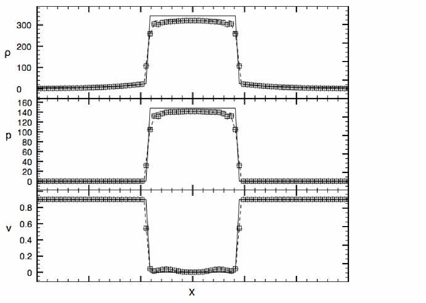
We first study a test problem with uniform grid in Cartesian coordinate that has been used by several groups to test the symmetric properties of a three-dimensional SRHD code (Aloy et al., 1999; Mignone et al., 2005). The initial setup of this test consists of a cold spherical inflow with initially constant density and constant velocity colliding at the box center. This problem is run using three-dimensional Cartesian coordinates so it allows one to evaluate the symmetry properties of the code (Marti et al., 1997; Aloy et al., 1999; Mignone et al., 2005). When gas collides at the center, a reflection shock forms. Behind the shock, the kinetic energy will be converted completely into internal energy. Thus the downstream velocity is zero and the specific internal energy is given by the upstream specific kinetic energy
| (26) |
Using the shock jump condition, the compression ratio and the shock velocity can be found to be
| (27) | |||
| (28) |
In the unshocked region (), the gas flow will develop a self-similar density distribution,
| (29) |
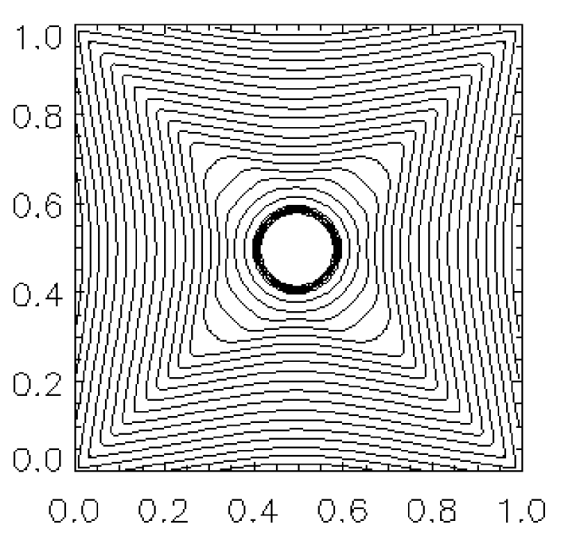
The initial state are . We chose a small value for pressure because a grid-based code cannot handle zero pressure. A CFL number is used for this problem, as other groups (Aloy et al., 1999). We chose to use LLF-PLM for this problem because this turns out to be the most stable solver for this problem. Fig. 17 shows the one-dimensional cut though axis and diagonal direction and Fig. 18 shows a contour through plane, both at . It can be seen from those plots that our code keeps the original spherical symmetry quite well. Since in a Cartesian box the simple outflow boundary condition is inconsistent with the initial spherical inflow setup, we evolve this problem only to , at which point all the mass in the original box has just entered the shocked region (see Fig. 17). After that time, the evolution would be affected by the unphysical boundary condition.
5.3.2 Relativistic Blast Wave I
In this test, we study a spherical blast wave in three-dimensional Cartesian coordinates. There is no analytical solution for this problem. Thus for the sake of comparison, we set up the same problem as other groups (Del Zanna & Bucciantini, 2002; Zhang & MacFadyen, 2006). The center of the blast wave source is located at the corner of the box. The initial conditions are
| (30) | |||
where is the distance to the center .
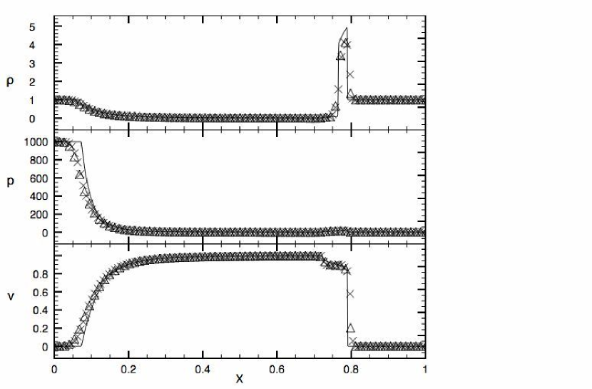
An ideal gas with an adiabatic index of is assumed. The left boundaries at x, y, z directions are reflecting while others are outflow. We use a top grid of zones with two more levels of refinement and a refinement factor of 2 for this calculation (equivalent resolution ). F-PLM is used for the result shown and the CFL number is .
The results are given in Fig. 19 which shows the cut along x-axis and diagonal direction. For comparison, we run a high resolution one-dimensional simulation using spherical coordinates. The three-dimensional run in Cartesian coordinates agrees with the one-dimensional high resolution run. Furthermore, it can be seen that the spherical symmetry of the initial condition is preserved rather well in the three-dimensional Cartesian case.
5.3.3 Relativistic Blast Wave II
Finally we study another blast wave problem for which the center of the blast wave source is located at the box center. This problem also does not have analytical solution but it has been studied by (Hughes et al., 2002) so our result can be compared to theirs. The initial conditions are
| (31) | |||
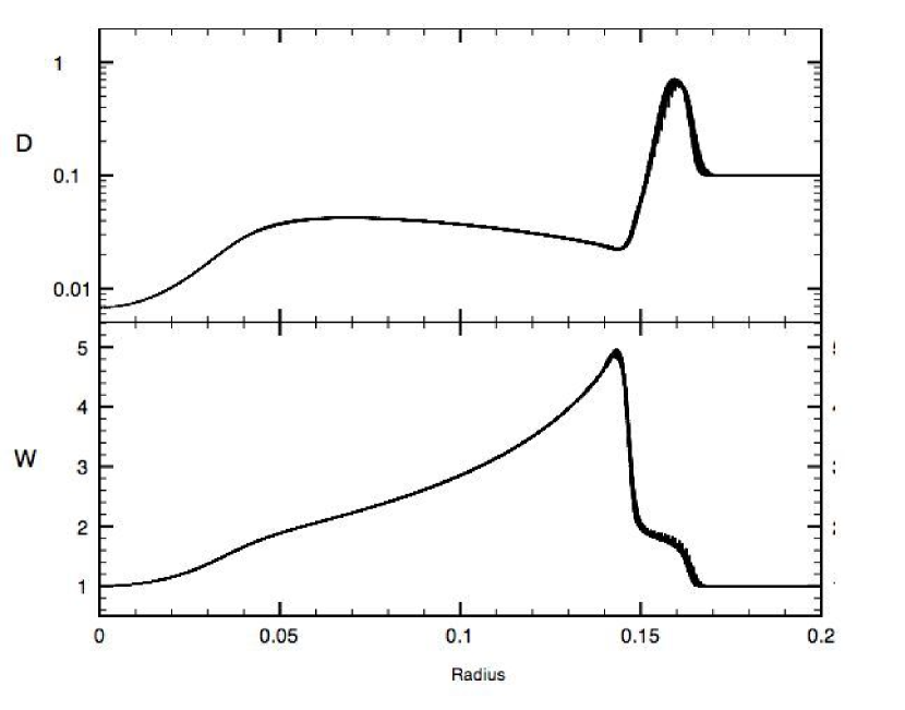
An ideal gas EOS with an adiabatic index of is used. We stop the run at , roughly the same ending time of Hughes et al. (2002). A top grid of zones with four levels of refinement and a refinement factor of two is used (equivalent resolution ). Thus our resolution is roughly times of Hughes et al. (2002). We used HLL-PLM and a CFL number of for this calculation.
Fig. 20 plots the numerical solution for all cells centered on the highest level in the two dimensional slice at at as a function of radius from the center (0.5,0.5,0.5). The position and amplitude of the high density shell agrees with the calculation of Hughes et al. (2002). And it can be seen that the spherical symmetry is preserved rather well in our code.
6. Astrophysical Application I Relativistic Supersonic Jet Propagation
Having validated our code using various test problems, we can apply it to astrophysical problems. We will study two typical astrophysical relativistic flow problems in this work, AGN jets and GRB jets. Both topics have been studied extensively with 2d simulations before, but very few 3d calculations have been done in both cases. Consequently we will focus on 3d simulations here.
In this section, we study a relativistic supersonic jet in three dimensions. We set up the problem using the same parameters as model C2 of (Marti et al., 1997). This model has also been studied in two dimensions by Zhang & MacFadyen (2006) and in three dimensions by Aloy et al. (1999). The jet parameters are , and . The jet has a classical Mach number so the pressure is . The parameters for the medium are , and . The EOS is assumed to be ideal with . The jet is injected from the low-z boundary centered at with radius . Outflow boundary conditions are used at other part of the boundary.
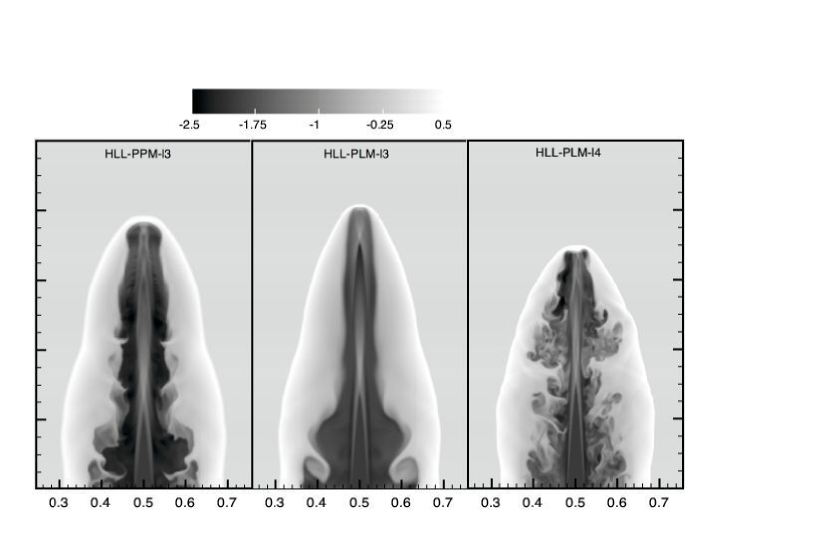
Figure 21 shows the result at for the three runs: HLL-PPM with three levels of refinement (HLL-PPM-l3), HLL-PLM with three levels of refinement (HLL-PLM-l3) and HLL-PLM with four levels of refinement (HLL-PLM-l4). The top grid resolution is zones. Thus the first two runs have an equivalent resolution of zones while the last one has zones. For the first two, turbulence in cocoon is not fully developed so the cocoon is still symmetric even in 3d. The HLL-PPM-l3 run has slightly more turbulent cocoon due to the higher spatial reconstruction order of PPM. Thus the HLL-PPM-l3 jet propagates slightly slower than the HLL-PLM-l3 jet. On the other hand, for the HLL-PLM-l4 jet, the resolution is cells per beam radius, comparable to the resolution used in the two-dimensional study by Marti et al. (1997). The cocoon turbulence is much more developed in this case, as in the 2d case (Marti et al., 1997). Consequently, the HLL-PLM-l4 jet propagates slower than the two lower resolution ones. Furthermore, the HLL-PLM-l4 case does not show axisymmetry because instability quickly develops in the lateral motion and consequently lateral motion also becomes turbulent.
Since we found the jet-cocoon structure differs significantly at higher resolution run and consequently the jet propagation speed decreases, we conclude that even at effective resolution of our three dimensional jet simulations the correct solution remains elusive. Moreover, different solvers give disparate answers.
7. Astrophysical Application II. Three Dimensional Simulation of Collapsar Jets
The idea that “long-soft” gamma-ray bursts are associated with the deaths of massive stars has been supported by various observations recently (see e.g. Woosley & Bloom (2006) for a recent review). So it is of great interest to calculate how a relativistic jet propagate through and break out of a massive star. There has been extensive calculations in 2d recently (Zhang et al., 2003, 2004; Mizuta et al., 2006; Morsony et al., 2006). But very few 3d calculation have been reported in the literature so far. Since there are significant turbulent motion and mixing in the jet-cocoon system in 2d calculation, it is important to model this process in 3d.
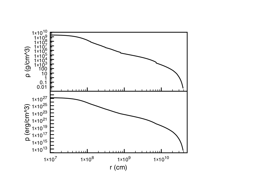
We use the projenitor HE16A of Woosley & Heger (2006), which is a stripped-down helium core with initial mass M⊙. Fig. 22 shows the density and pressure profiles for the progenitor model. The radius of the star at onset of collapse is cm. In our simulation, the mass inside cm is removed and replaced by a point mass of M⊙. The jet has power erg s-1, initial Lorentz factor , the ratio of its total energy (excluding rest mass energy) to its kinetic energy . This corresponds to a a jet with initial density g cm-3 and pressure erg cm-3. The jet is injected parallel to the axis with an initial radius cm. Those model parameters are similar to previous 2d calculations (Zhang et al., 2004; Mizuta et al., 2006).
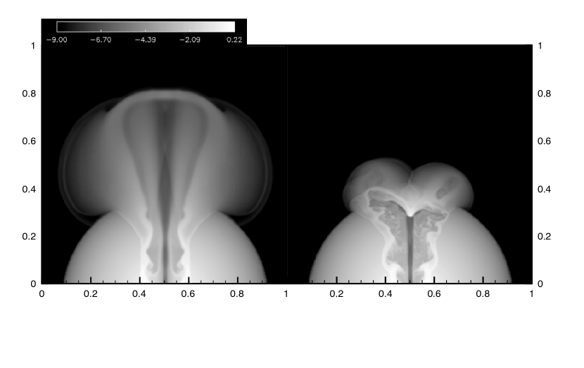
We use a simulation box of cm in order to follow the propagation of the jet after break out. We use HLL-PLM as this should be the most stable and reliable scheme to carry out resolution study. The top grid resolution is . We run the simulation using both 4 and 5 refinement levels, which correspond to resolution of 5.6 and 11 cells per jet beam radius, respectively. In order to always have high resolution for the jet material, we designed a color field refinement strategy in addition to the standard refinement criterion designed for discontinuities. More specifically, we use two color fields to keep track of the injected jet material and the stellar material. Those two color fields give us a fraction of jet material at every cell. Then whenever a cell contains more than 0.1 percent of jet material, we flag that cell for refinement. This ensures that we also have high resolution when mixing between jet material and star material happens.
The results for those two runs are show in Fig. 23. It can been seen that the high resolution run gives qualitatively different jet dynamics. While in the low resolution run the jet break out of the star successfully, in the high resolution run the jet head bifurcate at the stellar edge. Interestingly, this behavior has also been seen in 2d calculation (Morsony et al., 2006). But since we did not get convergent behavior so far, we cannot conclude at this stage whether this behavior is physical or purely numerical. However, it is safe to conclude that much higher resolution will be needed to model the jet break out in 3d.
8. Conclusions and Discussions
In this paper, we have described a new code that solves the special relativistic hydrodynamics equations with both spatially and temporally adaptive mesh refinement. It includes direct flux reconstruction and four approximate Riemann solvers including HLLC, HLL, LLF and modified Marquina flux formula. It contains several reconstruction routines: PLM, PPM, third order CENO, and third and fifth order WENO schemes. A modular code structure makes it easy to include more physics modules and new algorithms.
From our test problems and two astrophysical applications, it is clear that relativistic flow problems are more difficult than the Newtonian case. One key reason is that in the presence of utrarelativistic speed, nonlinear structures such as shocked shells are typically much thinner and thus requires the use of very high spatial resolution. SRHD problems also become difficult to solve accurately when significant transverse velocities are present in the problem as we have shown using several one dimensional problems. One reason for this difficulty is that in SRHD velocity components are coupled nonlinearly via the Lorentz factor. In studying astrophysical jet problems, we have demonstrated the need of both high resolution achievable only through AMR and careful choice of hydrodynamic algorithms. In addition to validate our AMR code, the most important implications of the calculations we have done is that in relativisitic flow simulations, resolution studies are crucial.
References
- Abel et al. (2002) Abel, T., Bryan, G. & Norman, M., 2002, Science, 295, 93
- Aloy et al. (1999) Aloy, M.-A., Ibáñez, J. M., Martí, J. M. & Müller, E. 1999, ApJS, 122, 151
- Aloy & Rezzolla (2006) Aloy, M. A., & Rezzolla, L. 2006, ApJ, 640, L115
- Anile (1989) Anile, A. M., 1989, Relativistic Fluids and Magnetofluids, Cambridge University Press, Cambridge, U.K.
- Anninos et al. (2005) Anninos, P., Fragile, P. C., & Salmonson, J. D. 2005, ApJ, 635, 723
- Begelman et al. (1984) Begelman, M. C., Blandford, R. D. & Rees, M. J. 1984, Rev. Mod. Phys., 56, 255
- Berger & Colella (1989) Berger, M. J., & Colella, P. 1989, J. Comput. Phys., 82, 64
- Berger & Oliger (1984) Berger, M. J. & Oliger, J. 1984, J. Comput. Phys., 53, 484
- Blandford et al. (1977) Blandford, R. D., McKee, C. F., & Rees, M. J. 1977, Nature, 267, 211
- Bryan & Norman (1997a) Bryan, G. L. & Norman, M. L. 1997a, arXiv:astro-ph/9710187
- Bryan & Norman (1997b) Bryan, G. L. & Norman, M. L. 1997b, ASP Conf. Ser. 123: Computational Astrophysics; 12th Kingston Meeting on Theoretical Astrophysics, 123, 363
- Bryan et al. (2001) Bryan, G. L., Abel, T., & Norman, M. L. 2001, arXiv:astro-ph/0112089
- Centrella & Wilson (1984) Centrella, J. & Wilson, J. R. 1984, ApJS, 54, 229
- Colella & Woodward (1984) Colella, P. & Woodward, P. R. 1984, J. Comput. Phys., 54, 174
- Del Zanna & Bucciantini (2002) Del Zanna, L. & Bucciantini, N. 2002, A&A, 390, 1177
- Donat et al. (1998) Donat, R., Font, J. A., Ibáñez, J. M. & Marquina, A. 1998, J. Comput. Phys., 146, 58
- Gehrels et al. (2004) Gehrels, N. et al. 2004, ApJ, 611, 1005
- Gingold & Monaghan (1977) Gingold, R. A., & Monaghan, J. J. 1977, MNRAS, 181, 375
- Harten et al. (1983) Harten, A., Lax, P. D. & van Leer, B. 1983, SIAM Rev., 25, 35
- Hawley et al. (1984a) Hawley, J. F., Wilson, J. R., & Smarr, L. L. 1984, ApJ, 277, 296
- Hawley et al. (1984b) Hawley, J. F., Wilson, J. R., & Smarr, L. L. 1984, ApJS, 55, 211
- Hughes et al. (2002) Hughes, P. A., Miller, M. A., & Duncan, G. C. 2002, ApJ, 572, 713
- Jiang & Shu (1996) Jiang, G.-S. & Shu, C.-W. 1996, J. Comput. Phys., 126, 202
- Kurganov & Tadmor (2000) Kurganov, A. & Tadmor, E. 2000, J. Comput. Phys., 160, 241
- Kurganov et al. (2001) Kurganov, A., Noelle, S. & Petrova, G. 2001, SIAM J. Sci. Comput., 23, 707
- LeVeque (2002) LeVeque, R. J. 2002, Finite Volume Methods for Hyperbolic Problems (Cambridge University Press)
- Lithwick & Sari (2001) Lithwick, Y. & Sari, R. 2001, ApJ, 555, 540
- Liu & Osher (1998) Liu, X.-D. & Osher, S. 1998, J. Comput. Phys., 142, 304
- Lucas-Serrano et al. (2004) Lucas-Serrano, A., Font, J. A., Ibáñez, J. M., & Martí, J. M. 2004, A&A, 428, 703
- Lucy (1977) Lucy, L. B. 1977, ApJ, 82, 1013
- Martí & Müller (1994) Martí, J. M. & Müller, E. 1994, J. Fluid Mech., 258, 317
- Martí & Müller (1996) Martí, J. M. & Müller, E. 1996, J. Comput. Phys., 123, 1
- Marti et al. (1997) Marti, J. M. A., Mueller, E., Font, J. A., Ibanez, J. M. A., & Marquina, A. 1997, ApJ, 479, 151
- Martí & Müller (2003) Martí, J. M. & Müller, E. 2003, Living Reviews in Relativity, 6, 7
- Meliani et al. (2007) Meliani, Z., Keppens, R., Casse, F. & Giannios, D. 2006, ArXiv preprint: astro-ph/0701434
- Mignone & Bodo (2005) Mignone, A. & Bodo, G. 2005, MNRAS, 364, 126
- Mignone et al. (2005) Mignone, A., Plewa, T., & Bodo, G. 2005, ApJS, 160, 199
- Mirabel & Rodriguez (1994) Mirabel, I. F. & Rodriguez, L. F. 1994, Nature, 371, 46
- Mizuta et al. (2006) Mizuta, A., Yamasaki, T., Nagataki, S., & Mineshige, S. 2006, ApJ, 651, 960
- Morsony et al. (2006) Morsony, B. J., Lazzati, D., & Begelman, M. C. 2006, ArXiv Astrophysics e-prints, arXiv:astro-ph/0609254
- Norman & Winkler (1986) Norman, M. L., & Winkler, K.-H. A. 1986, NATO Advanced Research Workshop on Astrophysical Radiation Hydrodynamics, 449, Eds. Karl-Heinz A. Winkler, Michael L. Norman
- O’Shea et al. (2004) O’Shea, B. W., Bryan, G., Bordner, J., Norman, M. L., Abel, T., Harkness, R., & Kritsuk, A. 2004, In ”Adaptive Mesh Refinement - Theory and Applications”, Eds. T. Plewa, T. Linde & V. G. Weirs, Springer Lecture Notes in Computational Science and Engineering, 2004
- Quirk (1994) Quirk, J. 1994, Int. J. Numer. Methods Fluids, 18, 555
- Pons et al. (2000) Pons, J. A., Martí, J. M. & Müller, E. 2000, J. Fluid Mech., 422, 125
- Schneider et al. (1993) Schneider, V., Katscher, U., Rischke, D. H., Waldhauser, B., Maruhn, J. A. & Munz, C.-D. 1993, J. Comput. Phys., 105, 92
- Shu & Osher (1988) Shu, C.-W. & Osher, S., 1988, J. Comput. Phys., 77, 439
- Tingay et al. (1995) Tingay, S. J. et al. 1995, Nature, 374, 141.
- Toro et al. (1994) Toro E. F., Spruce M. & Speares W. 1994, Shock Waves, 4, 25
- Van Leer (1977) Van Leer, B. 1977, J. Comput. Phys., 23, 276
- Van Leer (1979) Van Leer, B. 1979, J. Comput. Phys., 32, 101
- Wilson (1972) Wilson, J. R. 1972, ApJ, 173, 431
- Woosley & Bloom (2006) Woosley, S. E., & Bloom, J. S., 2006, ARAA, 44, 507
- Woosley & Heger (2006) Woosley, S. E., & Heger, A. 2006, ApJ, 637, 914
- Zhang & MacFadyen (2006) Zhang, W. & MacFadyen, A. I. 2006, ApJS, 164, 255
- Zhang et al. (2004) Zhang, W., Woosley, S. E., & Heger, A. 2004, ApJ, 608, 365
- Zhang et al. (2003) Zhang, W., Woosley, S. E., & MacFadyen, A. I. 2003, ApJ, 586, 356