Statefinder diagnostic for the modified polytropic Cardassian universe

Abstract

We apply the statefinder diagnostic to the modified polytropic Cardassian universe in this work. We find that the statefinder diagnostic is quite effective to distinguish Cardassian models from a series of other cosmological models. The $s-r$ plane is used to classify the modified polytropic Cardassian models into six cases. The evolutionary trajectories in the $s-r$ plane for the cases with different $n$ and $\beta$ reveal different evolutionary properties of the universe. In addition, we combine the observational $H(z)$ data, the cosmic microwave background data and the baryonic acoustic oscillation data to make a joint analysis. We find that Case 2 can be excluded at the 68.3% confidence level and any case is consistent with the observations at the 95.4% confidence level.

I Introduction

Recent type Ia Supernova observations, along with other observations such as cosmic microwave background (CMB) and galaxy power spectra, support the fact that the present expansion of our universe is accelerating Riess ; Perlmutter . In order to explain the accelerated expansion of the universe, cosmologists have tried to explore many cosmological models. A negative pressure term called dark energy is always taken into account, such as the cosmological constant model with equation of state $\omega_{\rm DE}=p_{\rm DE}/\rho_{\rm DE}=-1$ where $p_{\rm DE}$ and $\rho_{\rm DE}$ are pressure and density of the dark energy, respectively Carroll , the quiessence whose equation of state $\omega_{\rm Q}$ is a constant between -1 and -1/3 Alam , and the quintessence which is described in terms of a scalar field $\phi$ Caldwell ; Sahni1 . Some other candidates are constructed in different ways, such as the braneworld models which explain the acceleration through the fact that the general relativity is formulated in 5 dimensions instead of the usual 4 Csaki , and the Cardassian models which investigate the acceleration of the universe by a modification to the Friedmann-Robertson-Walker (FRW) equation Freese . In these cases, the dark energy component is not involved, but the accelerated expansion can still be obtained. The quantity $\omega_{\rm eff}$ is usually described as an effective equation of state for these models, and can be expressed by the Hubble parameter $H$ and its derivatives with respect to redshift $z$ Alam .

As so many cosmological models have been developed, a discrimination between these contenders becomes necessary. In order to achieve this aim, Sahni et al. proposed a new geometrical diagnostic named the statefinder pair $\{r,s\}$, where $r$ is generated from the scalar factor $a$ and its derivatives with respect to the cosmic time $t$, just as the Hubble parameter $H$ and the deceleration parameter $q$, and $s$ is a simple combination of $r$ and $q$ Sahni2 . The statefinder pair has been used to discriminate a series of cosmological models, including the LCDM universe with a cosmological constant $\Lambda$ and a cold dark matter term (CDM), the Chaplygin gas, the holographic dark energy models, the quintessence, the braneworld models and so on. Clear differences for the evolutionary trajectories in the $s-r$ plane have been found.

In this paper, we apply the statefinder diagnostic to the modified polytropic Cardassian universe. The original Cardassian model based on two parameters $\Omega_{m0}$ and $n$ was first suggested by Freese & Lewis Freese . It was generated from a modification to the Friedmann equation. Such a universe is spatially flat and accelerating today. But it involves no dark energy term and is dominated by merely matter and radiation. These Cardassian models predict the same distance-redshift relation as generic quintessence models, although they generate from completely different physical principles. A generalized Cardassian model–the modified polytropic Cardassian universe can be obtained by introducing an additional parameter $\beta$ into this model Gondolo1 ; Gondolo2 ; Wang , which reduces to the original model if $\beta=1$. The distance-redshift relation predictions of generalized Cardassian models can be very different from generic quintessence models, and can be differentiated with data from surveys of Type Ia Supernovae such as SuperNova/Acceleration Probe (SNAP). In all, the modified polytropic Cardassian universe can predict more fresh physical information than the original Cardassian. It is worthy of more detailed discussions.

In this work, we successfully classify the modified polytropic Cardassian models into six cases by the statefinder diagnostic. The cases with different $n$ and $\beta$ correspond to different evolutionary trajectories in the $s-r$ plane. The fact that LCDM corresponds to a fixed point (0, 1) in the $s-r$ plane plays a significant role for our classification. Also, it is very important to find where the evolutionary trajectories start and end. Another key standpoint is whether the evolutionary trajectory has a crossing with LCDM. We also study the relation between $(n,\beta)$ and the crossing redshift $z_{\rm C}$, at which the modified polytropic Cardassian universe intersects with LCDM in the $s-r$ plane. We find that the modified polytropic Cardassian models can be distinguished from other independent cosmological models by the statefinder diagnostic.

In addition, we use the observational $H(z)$ data derived from ages of the passively evolving galaxies Simon , the newly measured value of the CMB shift parameter $\mathcal{R}$ Odman and the $\mathcal{A}$-parameter which describes the baryonic acoustic oscillation (BAO) peak Eisenstein to make a combinational constraint. We assume a prior of $H_{0}=72\pm 8$ suggested by the Hubble Space Telescope (HST) Key Project Freedmann . From the confidence regions, we find that Case 2 is not consistent with the observations at the 68.3% confidence level and all the six cases do not conflict with the observations at the 95.4% confidence level.

This paper is organized as follows: In Sec.2, we briefly review the modified polytropic Cardassian universe. In Sec.3, we introduce the statefinder pair $\{r,s\}$. In Sec.4, we apply the statefinder diagnostic to various Cardassian models. In Sec.5, we make a combinational constraint on the parameters of the modified polytropic Cardassian universe. In Sec.6, the discussions and the conclusions are given.

II The Modified Polytropic Cardassian Universe

Measurements of CMB suggest a flat geometry for our universe Halverson ; Netterfield . If we consider a spatially flat FRW universe, the basic equation can be written as

$$H^{2}=\frac{8\pi G}{3}\rho,$$ (1)

where $G$ is Newton’s universal gravitation constant and $\rho$ is the density of summation of both matter and vacuum energy. Freese & Lewis Freese proposed a model called the Cardassian universe by adding a term on the right side of Eq.(1),

$$H^{2}=\frac{8\pi G}{3}\rho_{\rm m}+B\rho_{\rm m}^{n},$$ (2)

where $n$ is assumed to satisfy $n<2/3$ and $\rho_{\rm m}$ is always taken as a contribution of only the matter (in this paper we do not plan to consider radiation). If $n=0$, it is identical to the cosmological constant universe. If $B=0$, it reduces to the usual FRW equation, but with density of only matter. Thus, it is easy to get a new expression of $H$ from Eq.(2),

$$H^{2}=H_{\rm 0}^{2}[\Omega_{m0}(1+z)^{3}+(1-\Omega_{m0})(1+z)^{3n}],$$ (3)

by using

$$\rho_{\rm m}=\rho_{\rm m0}(1+z)^{3}=\Omega_{m0}\rho_{\rm c}(1+z)^{3},$$ (4)

where $\rho_{\rm m0}$ is current value of $\rho_{\rm m}$ and $\rho_{\rm c}=3H_{\rm 0}^{2}/8\pi G$ is the critical density of the universe. Clearly, this model predict the same distance-redshift relation as the quiessence with $\omega_{\rm Q}=n-1$. But we notice that they have completely different essentials. The quiessence requires a dark energy component while the Cardassian does not.

In the earlier time, the universe is dominated by the first term in Eq.(3) and the ordinary FRW behavior works. The additional term which consists of only matter gradually becomes a dominant driver afterwards. This transition was found to occur at $z\sim\emph{O}(1)$ Freese . Then the universe is caused to accelerate. The period of acceleration for this model is usually called the Cardassian era. The Cardassian model is attractive because the universe is flat and accelerating today but no vacuum energy is involved. And it has been demonstrated compatible with a series of observational tests, including the CMB data, the age of the universe, the structure formation and the cluster baryon fraction Freese .

The modified polytropic Cardassian universe can be obtained by introducing an additional parameter $\beta$ into the above model Gondolo1 ; Gondolo2 ; Wang ,

$$H^{2}=H_{\rm 0}^{2}[\Omega_{m\rm 0}(1+z)^{3}+(1-\Omega_{m\rm 0})f_{\rm X}(z)],$$ (5)

where

$$f_{\rm X}(z)=\frac{\Omega_{m\rm 0}}{1-\Omega_{m\rm 0}}(1+z)^{3}[(1+\frac{\Omega_{m\rm 0}^{-\beta}-1}{(1+z)^{3(1-n)\beta}})^{1/\beta}-1].$$ (6)

The two parameters $(n,\beta)$ are usually taken as $n<2/3$ and $\beta>0$. If $\beta=1$, the model reduces to the original one characterized by Eq.(3) while if $f_{\rm X}(z)=1$, the model just corresponds to LCDM.

Similar to Wang et al., we also take $\Omega_{m\rm 0}=0.3$ as a prior in subsequent discussions. In the work of Wang et al., this model was compared with current supernova data and CMB data. It was proved that the existing data can be well fit for several chosen values of $n$ and $\beta$. Also, the simulated data were constructed to make a discrimination between the modified polytropic Cardassian universe and LCDM as well as the quintessence. Once $\Omega_{m\rm 0}$ is known with an accuracy of 10%, SNAP can determine the sign of the time dependence of dark energy density which provides a first discrimination between various cosmological models Wang . In this work, we use a geometrical tool-the statefinder diagnostic to make a classification and a discrimination about the modified polytropic Cardassian models.

III A Brief Overview of the Statefinder Diagnostic

The Hubble parameter $H=\dot{a}/a$ and the deceleration parameter $q=-\ddot{a}/aH^{2}$ are two traditional geometrical diagnostics. They only depend on the scalar factor $a$ and its derivatives with respect to $t$, i.e., $\dot{a}$ and $\ddot{a}$. Through $a=1/(1+z)$, the deceleration parameter $q$ can be expressed as

$$q(z)=\frac{H^{\prime}}{H}(1+z)-1,$$ (7)

where $H^{\prime}$ is the derivative of $H$ with respect to redshift $z$. The deceleration parameter $q$ is a good choice to describe the expansion state of our universe, but it is not perfect enough to characterize the cosmological models uniquely. This shortage can be easily seen from the fact that many models may correspond to the same current value of $q$. And this difficulty can be overcome by another geometrical diagnostic–the statefinder pair $\{r,s\}$. This approach has been used to distinguish a series of cosmological models successfully.

For a spatially flat universe, the statefinder $r$ is defined as follows Sahni2

$$r=\frac{\stackrel{{\scriptstyle\cdots}}{{a}}}{aH^{3}},$$ (8)

where $\stackrel{{\scriptstyle\cdots}}{{a}}$ is the third derivative of $a$ with respect to $t$. $s$ is just a combination of $r$ and $q$,

$$s=\frac{r-1}{3(q-1/2)}.$$ (9)

The statefinder pair was first introduced to analyze a flat universe with a cold matter and a dark energy term. For these contenders, $r$ is given by

$$r=1+\frac{9}{2}\omega_{\rm DE}(1+\omega_{\rm DE})\Omega_{\rm DE}-\frac{3}{2}\frac{\dot{\omega}_{\rm DE}}{H}\Omega_{\rm DE}.$$ (10)

where $\Omega_{\rm DE}=\rho_{\rm DE}/\rho_{\rm c}$ and $\dot{\omega}_{\rm DE}$ is the derivative of $\omega_{\rm DE}$ with respect to $t$. And the other diagnostic,

$$s=1+\omega_{\rm DE}-\frac{1}{3}\frac{\dot{\omega}_{\rm DE}}{\omega_{\rm DE}H}.$$ (11)

From the two equations above it is easy to realize that LCDM corresponds to a fixed point (0, 1) in the $s-r$ plane and the standard cold dark matter (SCDM) universe with no dark energy term locates at (1, 1) forever. For this particularity, the current values of $\{r,s\}$ provide a considerable way to measure the distance from a specific model to LCDM.

More generally, $r$ and $s$ can be given in terms of the Hubble parameter $H$ and its first and second derivatives $H^{\prime}$ and $H^{\prime\prime}$ with respect to redshift $z$,

$$r(z)=1-2\frac{H^{\prime}}{H}(1+z)+{\frac{H^{\prime\prime}}{H}+(\frac{H^{\prime}}{H})^{2}},$$ (12)

$$s(z)=\frac{-2H^{\prime}(1+z)/H+{H^{\prime\prime}/H+(H^{\prime}/H)^{2}}}{3(H^{{}^{\prime}}(1+z)/H-3/2)}.$$ (13)

Thus we can use the new tool to describe the evolutionary trajectories of the modified polytropic Cardassian universe.

IV The $s-r$ Plane for Modified Polytropic Cardassian Universe

For the original Cardassian model with $\beta=1$, it corresponds to a compatible expression with the quiessence with $\omega_{\rm Q}=n-1$. The quiessence has been studied using the statefinder diagnostic in several literatures Alam ; Sahni2 . In the $s-r$ plane, a vertical line with $s=n$ and $r$ changing monotonically from 1 to $1+9n(n-1)/2$ represents the evolutionary trajectory of the universe.

For cases with $\beta\neq 1$, we first pay our attention to the epoches in the far past $(a\to 0)$ and the far future $(a\to+\infty)$. It is clear that $z\to+\infty$ represents the former case and $z\to-1$ stands for the latter. From Eq.(12), it is easy to find the limit condition

$$\lim_{z\to+\infty}r(z)=1,$$ (14)

which means that the value of $r$ in the far past is independent on $n$ and $\beta$. However, we can not derive the similar properties for the value of $s$ from Eq.(13). It is related to both of $n$ and $\beta$. For the limit of $z\to-1$, from Eq.(12), we get

$$\lim_{z\to-1}r(z)=1+\frac{9}{2}n(n-1).$$ (15)

And from Eq.(13), we have

$$\lim_{z\to-1}s(z)=n.$$ (16)

The values of both $s$ and $r$ are independent on $\beta$.

Generally, some models have a crossing with LCDM in the $s-r$ plane. By substituting the Hubble parameter, Eq.(5), in the expressions of $r$ and $s$, Eq.(12) and Eq.(13), we find that the crossing with LCDM happens at the redshift

$$z_{\rm C}=[(\Omega_{\rm m0}^{-\beta}-1)\frac{-n}{1-\beta+n\beta}]^{\frac{1}{3(1-n)\beta}}-1.$$ (17)

And we notice that the crossing can happen only if the following inequality is satisfied,

$$(\Omega_{\rm m0}^{-\beta}-1)\frac{-n}{1-\beta+n\beta}\geq 0.$$ (18)

Due to the prior $\Omega_{\rm m0}=0.3$ and $\beta>0$, $\Omega_{\rm m0}^{-\beta}-1>0$ is naturally satisfied. Thus we may describe the condition in Eq.(18) equivalently as

$$\frac{n}{1-\beta+n\beta}\leq 0.$$ (19)

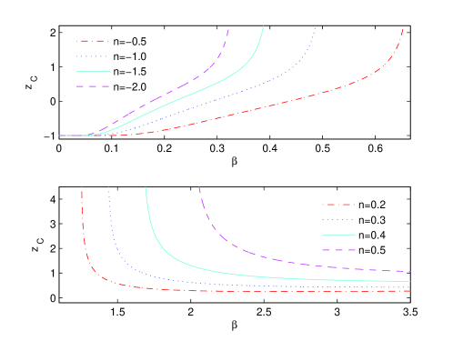
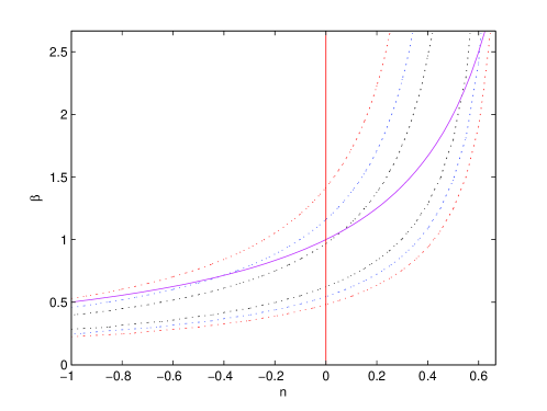
In order to understand the relation among $n$, $\beta$ and $z_{\rm C}$ clearly, we draw a $\beta-z_{\rm C}$ plane for several fixed $n$ in Fig.1. For $n>0$, the crossing takes place at $z_{\rm C}>0$ for any $\beta$, and $z_{\rm C}$ changes little for larger values of $\beta$. For $n<0$, whether $z_{\rm C}>0$ or $z_{\rm C}<0$ depends on the values of $\beta$. And $z_{\rm C}$ is nearly equal to -1 if $\beta$ is small enough. For the particular case which satisfies $1-\beta+n\beta=0$, the expected crossing happens at $z_{\rm C}\to\infty$. Clearly, $n=0$ and $\beta=1/(1-n)$ are the two critical conditions.

Figure 1: $\beta-z_{\rm C}$ planes for $n$=-0.5, -1.0, -1.5 and -2.0 (the top panel) as well as $n$=0.2, 0.3, 0.4 and 0.5 (the bottom panel).

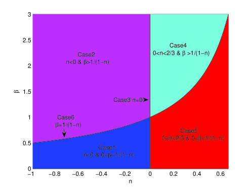
Now we use Eq.(19) to classify the modified polytropic Cardassian universe. We draw an $n-\beta$ plane in Fig.2 and divide it into different regions by the critical curves $n=0$ and $\beta=1/(1-n)$:

$$\left\{\begin{array}[]{llllll}{\textbf{Case 1}}&n<0\ {\rm and}\ 0<\beta<1/(1-n);\\ {\textbf{Case 2}}&n<0\ {\rm and}\ \beta>1/(1-n);\\ {\textbf{Case 3}}&n=0;\\ {\textbf{Case 4}}&0<n<2/3\ {\rm and}\ \beta>1/(1-n);\\ {\textbf{Case 5}}&0<n<2/3\ {\rm and}\ 0<\beta<1/(1-n);\\ {\textbf{Case 6}}&\beta=1/(1-n).\end{array}\right.$$ (20)

Figure 2: $n-\beta$ plane based on $n$ and $\beta$. The vertical solid line represents $n=0$ (Case 3), and the declined solid curve stands for $\beta=1/(1-n)$ (Case 6).

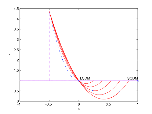
Case 1 ($n<0$ and $0<\beta<1/(1-n)$): $n$=-0.5, $\beta$=0.1, 0.2, 0.3, 0.4 and 0.5 are taken for a qualitative analysis. We plot the $s-r$ plane in Fig.3. Although the original Cardassian model with $\beta=1$ is not involved in this case, we still draw this curve for a comparison. All the curves start at $r=1$ and $0<s<1$ on the horizontal line, i.e., on the right of LCDM. After passing by LCDM, they arrive at their common end $(-0.5,4.38)$ in far future. And the crossing with LCDM happens at $z_{\rm C}$=-0.999, -0.84, -0.50, -0.13 and 0.25 for $\beta$=0.1, 0.2, 0.3, 0.4 and 0.5 respectively. Particularly, the fixed point (0, 1) for LCDM just is the beginning point for the critical case of $\beta=1/(1-n)=2/3$.

Figure 3: $s-r$ plane for Case 1. The star (0, 1) corresponds to LCDM, the star (1, 1) SCDM and other dots the current values of the Statefinder pair, i.e., $(s_{\rm 0},r_{\rm 0})$ (also for subsequent cases). And the solid curves from bottom to top correspond to the evolutionary trajectories of $n$=-0.5, $\beta$=0.1, 0.2, 0.3, 0.4 and 0.5 respectively. The dot-dash curves represent the critical case $\beta=2/3$. For a comparison, the vertical dashed line stands for the case of $\beta=1$.

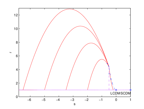
Case 2 ($n<0$ and $\beta>1/(1-n)$): To be consistent with Case 1, we consider $n=-0.5$ again, but $\beta$=0.8, 1, 2, 3, 4 and 5 respectively. The $s-r$ plane is plotted in Fig.4. The crossing with LCDM never occurs for this case. The vertical line $s=n$ for the evolutionary trajectory of $\beta=1$ divides the whole plane into two parts. The left part with $n<s<0$ stands for $1/(1-n)<\beta<1$ and the right part with $s<n$ corresponds to $\beta>1$. And all the evolutionary trajectories commence at one point with $r=1$. The same as Case 1, they arrive at $(-0.5,4.38)$ in the end.

Figure 4: $s-r$ plane for Case 2. The solid curves from right to left correspond to the evolutionary trajectories of $n$=-0.5, $\beta$=0.8, 2, 3, 4 and 5 respectively. And the vertical dashed line stands for the case of $\beta=1$. Same as Fig.3, the dot-dash curve represents the critical case $\beta=2/3$.

Case 3 ($n=0$): We plot the $s-r$ plane for $\beta$=0.3, 0.7, 1, 2, 3 and 4 in Fig.5 . One point with $r=1$ acts as the beginning point, and (0, 1) the common end. This diagram is divided into two segments by the LCDM fixed point, or equivalently the modified polytropic Cardassian model with $n=0$ and $\beta=1$. The segment with $r>1$ corresponds to $\beta>1$ while the other segment with $r<1$ corresponds to $\beta<1$.

Figure 5: $s-r$ plane for Case 3. The solid curves from bottom to top stand for $\beta$=0.3, 0.7, 2, 3 and 4 respectively. The case of $\beta=1$ just corresponds to the fixed point for LCDM, i.e., (0, 1).

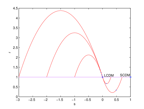
Case 4 ($0<n<2/3$ and $\beta>1/(1-n)$): The $s-r$ plane for $n=0.2$, $\beta$=2, 3, 4 and 5 is plotted in Fig.6. Clearly, all the curves start with $r=1$ and $s<0$, and then pass by LCDM after an arc route. All the latter evolutionary parts of the trajectories nearly overlap with each other. They are insensitive to $\beta$. The point $(0.2,0.28)$ is the common end. The crossing redshifts are not too far from each other for different values of $\beta$, i.e., $z_{\rm C}\simeq 0.3$. It is interesting that the fixed point (0, 1) for LCDM is just the beginning point for the critical case of $\beta=1/(1-n)=5/4$. And the Cardassian models for this case can satisfy the weak energy condition $\omega=p_{\rm X}/(\rho_{\rm m}+\rho_{\rm X})>-1$ although the effective equation of state satisfies $\omega_{\rm eff}=p_{\rm X}/\rho_{\rm X}<-1$. $w_{\rm eff}<-1$ is consistent with many observations such as CMB and large scale structure data (Schuecker, ; Melchiorri, ).

Figure 6: $s-r$ plane for Case 4. The solid curves from right to left stand for the evolutionary trajectories of $n=0.2$, $\beta$=2, 3, 4 and 5 respectively. The dot-dash curve represents the critical case $\beta=5/4$. For a comparison, the vertical dashed line stands for the case of $\beta=1$.

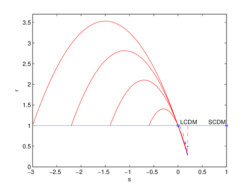
Case 5 ($0<n<2/3$ and $0<\beta<1/(1-n)$): Same as Case 4, $n=0.2$ is considered, but $\beta$=0.3, 0.6, 0.9, 1.0 and 1.1. We plot the $s-r$ plane in Fig.7. All the evolutionary trajectories start with $r=1$ and $s>0$. They arrive at $(0.2,0.28)$ in the end, and never pass by LCDM. The whole plane is divided into two parts by the vertical line $s=n$ (corresponding to the case of $\beta=1$). The left part satisfies $1<\beta<5/4$ and $\beta<1$ is satisfied for the right.

Figure 7: $s-r$ plane for Case 5. The solid curves from right to left correspond to the evolutionary trajectories of $n$=0.2, $\beta$=0.3, 0.6, 0.9 and 1.1 respectively. And the vertical dashed line stands for the case of $\beta=1$. Same as Fig.6, the dot-dash curve represents the critical case $\beta=5/4$.

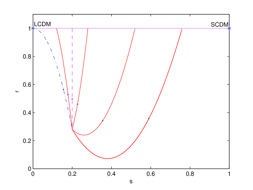
Case 6 ($\beta=1/(1-n)$): This is another critical case besides Case 3. $n$=-0.5, -0.4, -0.3, -0.2, -0.1, 0, 0.1, 0.2, 0.3, 0.4, 0.5, and 0.6 are considered. For this case, crossing with LCDM happens at $z_{\rm C}\to\infty$. We plot the $s-r$ plane in Fig.8. All the evolutionary trajectories start at LCDM in the past and end at $(-1+3n/2,1+9n(n-1)/2)$ in the future.

Figure 8: $s-r$ plane for Case 6. The point (0, 1) stands for $n=0$. Then $n$ increases by a interval of 0.1 until 0.6 for cases on the right of (0, 1) and $n$ decreases by a interval of 0.1 until -0.5 for cases on the left of (0, 1). The other vertical dashed lines stand for the evolutionary trajectories of cases with $\beta=1$ and different values of $n$.

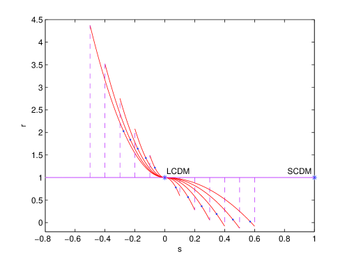
We have successfully given a qualitative analysis to the modified polytropic Cardassian universe from the statefinder viewpoint and it has been classified into six cases. A prior $\Omega_{\rm m0}=0.3$ is adopted in this work. We also take some other values of $\Omega_{\rm m0}$ for comparison and notice that $\Omega_{\rm m0}$ is not a sensitive parameter for our analysis in this work. And it has been clear that the $s-r$ plane is effective enough to discriminate the modified polytropic Cardassian models. The fact that LCDM corresponds to a fixed point (0, 1) in the $s-r$ plane plays a significant role for our classification. Whether the evolutionary trajectory has a crossing with LCDM is our basic standpoint. Also, the beginning points and the ending points are both key factors for shapes of the evolutionary trajectories.

V Data Analysis from Observational $H(z)$ Data, CMB and BAO

In order to understand the six cases above more clearly, we use the observational $H(z)$ data derived from the passively evolving galaxies, the cosmic microwave background (CMB) shift parameter $\mathcal{R}$ and the $\mathcal{A}$-parameter which describes the baryonic acoustic oscillation (BAO) peak to make a joint analysis.

The Hubble parameter $H(z)$ depends on the differential age of the universe in this form

$$H(z)=-\frac{1}{1+z}\frac{{\rm d}z}{{\rm d}t},$$ (21)

which provides a direct measurement for $H(z)$ through a determination of ${\rm d}z/{\rm d}t$. By using the differential ages of passively evolving galaxies determined from the Gemini Deep Deep Survey Abraham and archival data Treu ; Treu+ ; Nolan ; Nolan+ , Simon et al. determined a set of observational $H(z)$ data in the range $0\lesssim z\lesssim 1.8$ and used them to constrain the dark energy potential and its redshift dependence Simon . Yi & Zhang first first used them to analyze the holographic dark energy models and got a consistent result with others Yi .

The model-independent shift parameter $\mathcal{R}$ can be derived from CMB data. It is defined as Odman

$$\mathcal{R}=\sqrt{\Omega_{\rm m0}}\int_{0}^{z_{\rm r}}\frac{dz}{E(z)},$$ (22)

where $E(z)=H(z)/H_{0}$ and $z_{\rm r}=1089$ is the redshift of recombination. From the three-year result of WMAP Spergel , Wang & Mukherjee estimated $\mathcal{R}=1.70\pm 0.03$ Wang+ .

Using a large spectroscopic sample of 46748 luminous red galaxies covering 3816 square degrees out to $z=0.47$ from the Sloan Digital Sky Survey, Eisenstein et al. Eisenstein successfully found the acoustic peaks in the CMB anisotropy power spectrum, described by the model-independent $\mathcal{A}$-parameter,

$$\mathcal{A}=\sqrt{\Omega_{\rm m0}}[\frac{1}{z_{1}E^{1/2}(z_{1})}\int_{0}^{z_{1}}\frac{dz}{E(z)}]^{2/3},$$ (23)

where $z_{1}=0.35$ is the redshift at which the acoustic scale has been measured. Eisenstein et al. Eisenstein suggested the measured value of the $\mathcal{A}$-parameter as $\mathcal{A}=0.469\pm 0.017$.

The best-fit parameters of the modified polytropic Cardassian universe can be determined by minimizing

$$\chi^{2}=\sum_{i}\frac{[H_{\rm th}(z_{i})-H_{\rm ob}(z_{i})]^{2}}{\sigma_{i}^{2}}+\frac{(\mathcal{R}-1.70)^{2}}{0.03^{2}}+\frac{(\mathcal{A}-0.469)^{2}}{0.017^{2}},$$ (24)

where $H_{\rm th}(z_{i})$ is the theoretical Hubble parameter at $z_{i}$, $H_{\rm ob}(z_{i})$ is the observational Hubble parameter at $z_{i}$ and $\sigma_{i}$ is the corresponding $1\sigma$ error. We get the best-fit values $n=-1.85$ and $\beta=0.23$, with $\chi^{2}_{\rm min}=10.12$. The best-fit results correspond to Case 1. And the crossing with LCDM in the $s-r$ plane occurs at $z_{\rm C}$=0.32. The current values of the diagnostics are $s_{\rm 0}$=-0.19 and $r_{\rm 0}$=1.59. The confidence regions in the $n-\beta$ plane are plotted in Fig.9, from which we find that Case 2 can be excluded at the 68.3% confidence level and all the six cases are consistent with the observational data at the 95.4% confidence level.

Figure 9: Confidence regions in the $n-\beta$ plane for the joint analysis (the regions from inner to outer stand for confidence levels at 68.3%, 95.4% and 99.7% respectively). The vertical solid line represents $n=0$ (Case 3), and the declined solid curve stands for $\beta=1/(1-n)$ (Case 6).

VI Discussions and Conclusions

The statefinder diagnostic is powerful to discriminate various cosmological models. Differences of the evolutionary trajectories in the $s-r$ plane among a series of cosmological models have been found. For example, LCDM corresponds to a fixed point (0, 1) and the point (1, 1) represents SCDM. For the holographic dark energy model with $c=1$ Cohen , the curve in the $s-r$ plane commences at (2/3, 1) in the past and ends at LCDM in the future, with $s$ monotonically decreasing from 2/3 to 0 and $r$ first decreasing from 1 to a minimum value and then rising to 1 Zhang1 . Both the quintessence tracker models (with tracker potentials $V=V_{\rm 0}/\phi^{\alpha}$) and the Chaplygin gas models have arc evolutionary trajectories, but in different regions Alam ; Evans ; Gorini . The conditions $-1\leq s\leq 0$ and $r\leq 1$ are satisfied for the former cosmological model while $0\leq s\leq 1$ and $r\geq 1$ for the latter. The evolutionary trajectories of the coupled quintessence models have more complicated evolutionary properties Zhang2 . And quintessence models with other potentials were studied by Evans et al.Evans , also along with a generalization of $\{r,s\}$ to a non-flat universe.

Also, the $q-r$ plane has been widely used for discussion on the evolutionary property of the universe. For example, the point (0.5, 1) corresponds to SCDM in the $q-r$ plane and the horizontal straight line from (0.5, 1) to (-1, 1) stands for LCDM. The braneworld models have been studied too, including Disappearing Dark Energy (DDE) as the simplest case Alam . LCDM separates the first braneworld model (named BRANE1 in Alam and the effective equation of state satisfies $\omega_{\rm eff}\leq-1$) from the second braneworld model (named BRANE2 in Alam and the effective equation of state satisfies $\omega_{\rm eff}\geq-1$) and DDE models. DDE both begins and ends at SCDM, forming a loop. However, although both BRANE1 and BRANE2 commence their evolutions at (0.5, 1) and end at (-1, 1), the diagnostic $r$ satisfies $r\geq 1$ for BRANE1 while $r\leq 1$ for BRANE2.

As the $s-r$ plane has been found robust for our classification for the modified polytropic Cardassian models, we do not intend to make use of the $q-r$ plane. For the modified polytropic Cardassian universe, the evolutionary trajectories can be picked out easily with help of the $s-r$ plane if $\beta\neq 1$. In fact, the original Cardassian model with $\beta$=1 can not be discarded from the quiessence with $\omega_{\rm Q}=n-1$ because they correspond to identical expressions for both $r$ and $s$. Such a consistence has also been mentioned by Freese & Lewis, as well as how to distinguish the two models Freese .

Distinct differences in the $s-r$ plane have been realized for the cases with different $n$ and $\beta$ for the modified polytropic Cardassian universe. For Case 1 and Case 4, the crossing with LCDM happens at some $z_{\rm C}$, while the same state never occurs for Case 2 and Case 5. And Case 3 and Case 6 just are two critical cases. Also, the beginning points and the ending points are tightly related to the shapes of the evolutionary trajectories. They seriously depend on $n$ and $\beta$, especially $n$. As $n$ and $\beta$ are found to be sensitive to the modified polytropic Cardassian models, constraining the two parameters exactly becomes a valuable task. We use the observational $H(z)$ data, the CMB data and the BAO data to make a combinational constraint. We find that Case 2 can be excluded at the 68.3% confidence level and all the six cases are consistent with the observational data at the 95.4% confidence level. Recent other constraints suggest some results far from consistent with each other. For example, in the work of Wang et al., the choices of $n=0.2$, $\beta=1$; $n=0.2$, $\beta=2$ and $n=0.2$, $\beta=3$ are all consistent with SN Ia and CMB observations Wang . The first case corresponds to the quiessence with the equation of state $\omega_{\rm Q}=-0.8$, and this case is consistent with Case 5. The latter two cases with the crossing at $z_{\rm C}$=0.29 and 0.26 respectively are in agreement with Case 4. And the current values of the diagnostics are $s_{\rm 0}$=0.13, $r_{\rm 0}$=0.58 and $s_{\rm 0}$=0.16, $r_{\rm 0}$=0.45 for $n=0.2$, $\beta$=2 and $n=0.2$, $\beta$=3 respectively. Nesseris & Perivolaropoulos Nesseris suggested another result $n=-23_{-9}^{+8}$, $\beta=0.025_{-0.010}^{+0.008}$ with a supernova data set consisting of 194 SN Ia Tonry ; Barris . Both Case 1 and Case 2 may be included within the given error-bar. The best fitting values lie in Case 1 and the crossing with LCDM happens at $z_{\rm C}$=0.37. Meanwhile, the present quantities are $s_{\rm 0}$=-0.29 and $r_{\rm 0}$=1.94. Evans et al. provided a best fitting result $n=-0.94$ and $\beta=0.06$ with a simulated data set Evans . This result is in agreement with Case 1. The crossing happens in the far future, i.e., at $z_{\rm C}$=-0.999. And the current values $s_{\rm 0}$=0.76 and $r_{\rm 0}$=0.54 indicate a large distance from LCDM. As constraints still remain weak, we expect for data with higher precision to provide more consistent fitting results in future. We also hope theses statefinder parameters can be determined more exactly and shed light on the nature of the cosmological models.

VII Acknowledgments

We are very grateful to the anonymous referee for his valuable comments that greatly improve this paper. And we are also grateful to Xin Zhang for his helpful suggestions. Z. L. Yi would like to thank Qiang Yuan and Jie Zhou for their kind help. This work was supported by the National Science Foundation of China (Grants No.10473002 and 10273003), the Scientific Research Foundation for the Returned Overseas Chinese Scholars.

References

- (1) A. G. Riess, A. V. Filippenko, P. Challis, A. Clocchiattia, A. Diercks, P. M. Garnavich, R. L. Gilliland, C. J. Hogan, S. Jha, K. R. Kirshner, B. Leibundgut, M. M. Phillips, D. Reiss, B. P. Schmidt, R. A. Schommer, R. C. Smith, J. Spyromilio, C. Stubbs, N. B. Suntzeff and J. Tonry, Astron. J. 116, 1009 (1998).
- (2) S. Perlmutter, G. Aldering, G. Goldhaber, R. A. Knop, P. Nugent, P. G. Castro, S. Deustua, S. Fabbro, A. Goobar, D. E. Groom, I. M. Hook, A. G. Kim, M. Y. Kim, J. C. Lee, N. J. Nunes, R. Pain, C. R. Pennypacker, R. Quimby, C. Lidman, R. S. Ellis, M. Irwin, R. G. McMahon, P. Ruiz-Lapuente, N. Walton, B. Schaefer, B. J. Boyle, A. V. Filippenko, T. Matheson, A. S. Fruchter, N. Panagia, H. J. M. Newberg and W. J. Couch, Astrophys. J. 517, 565 (1999).
- (3) S. M. Carroll, W. H. Press and E. L. Turner, Annu. Rev. Astron. Astrophys. 30, 499 (1992).
- (4) U. Alam, V. Sahni, T. D. Saini and A. A. Starobinsky, Mon. Not. R. Astron. Soc. 344, 1057 (2003).
- (5) R. R. Caldwell, R. Dave and R. J. Steinhardt, Phys. Rev. Lett. 80, 1582 (1998).
- (6) V. Sahni and L. M. Wang, Phys. Rev. D 62, 103517 (2000).
- (7) C. Csaki, M. Graesser, L. Randall and J. Terning, Phys. Rev. D 62, 045015 (2000).
- (8) K. Freese and M. Lewis, Phys. Lett. B 540, 1 (2002).
- (9) V. Sahni, T. D. Saini, A. A. Starobinsky and U. Alam, JETP Lett. 77, 201 (2003).
- (10) P. Gondolo and K. Freese, Phys. Rev. D 68, 063509 (2003).
- (11) P. Gondolo and K. Freese, Phys. D hep-ph/0211397.
- (12) Y. Wang, K. Freese, P. Gondolo and M. Lewis, Astrophys. J. 594, 25 (2003).
- (13) J. Simon, L. Verde and R. Jimenez, Phys. Rev. D 71, 123001 (2005).
- (14) C. J. Odman, A. Melchiorri, M. P. Hobson and A. N. Lasenby, Phys. Rev. D 67, 083511 (2003).
- (15) D. J. Eisenstein, I. Zehavi, D. W. Hogg, R. Scoccimarro, M. R. Blanton, R. C. Nichol, R. Scranton, H. Seo, M. Tegmark, Z. Zheng, S. Anderson, J. Annis, N. Bahcall, J. Brinkmann, S. Burles, F. J. Castander, A. Connolly, I. Csabai, M. Doi, M. Fukugita, J. A. Frieman, K. Glazebrook, J. E. Gunn, J. S. Hendry, G. Hennessy, Z. Ivezic, S. Kent, G. R. Knapp, H. Lin, Y . Loh, R. H. Lupton, B. Margon, T. McKay, A. Meiksin, J. A. Munn, A. Pope, M. Richmond, D. Schlegel, D. Schneider, K. Shimasaku, C. Stoughton, M. Strauss, M. SubbaRao, A. S. Szalay, I. Szapudi, D. Tucker, B. Yanny and D. York, Astrophys. J. 633, 560 (2005).
- (16) W. L. Freedmann, B. F. Madore, B. K. Gibson, L. Ferrarese, D. D. Kelson, S. Sakai, J. R. Mould, R. C. Kennicutt, Jr., H. C. Ford, J. A. Graham, J. P. Huchra, S. M. G. Hughes, G. D. Illingworth, L. M. Macri and P. B. Stetson, Astrophys. J. 553, 47 (2001).
- (17) N. W. Halverson, E. M. Leitch, C. Pryke, J. Kovac, J. E. Carlstrom, W. L. Holzapfel, M. Dragovan, J. K. Cartwright, B. S. Mason, S. Padin, T. J. Pearson, M. C. Shepherd and A. C. S. Readhead, Astrophys. J. 568, 38 (2002).
- (18) C. B. Netterfield, P. A. R. Ade, J. J. Bock, J. R. Bond, J. Borrill, A. Boscaleri, K. Coble, C. R. Contaldi, B. P. Crill, P. de Bernardis, P. Farese, K. Ganga, M. Giacometti, E. Hivon, V. V. Hristov, A. Iacoangeli, A. H. Jaffe, W. C. Jones, A. E. Lange, L. Martinis, S. Masi, P. Mason, P. D. Mauskopf, A. Melchiorri, T. Montroy, E. Pascale, F. Piacentini, D. Pogosyan, F. Pongetti, S. Prunet, G. Romeo, J. E. Ruhl and F. Scaramuzzi, Astrophys. J. 571, 604 (2002).
- (19) P. Schuecker, R. R. Caldwell, H. Bohringer, C. A. Collins, L. Guzzo, N. N. Weinberg, Astron. Astrophys. 402, 53 (2003).
- (20) A. Melchiorri, L. Mersini, C. J. Odman and M. Trodden, Phys. Rev. D 68, 043509 (2003).
- (21) R. G. Abraham, K. Glazebrook, P. J. McCarthy, D. Crampton, R. Murowinski, I. Jorgensen, K. Roth, I. M. Hook, S. Savaglio, H. W. Chen, R. O. Marzke and R. G. Carlberg, Astron. J. 127, 2455 (2004).
- (22) T. Treu, P. Mller, M. Stiavelli, S. Casertano and G. Bertin, Astrophys. J. Lett. 564, L13 (2002).
- (23) T. Treu, M. Stiavelli, P. Mller, S. Casertano and G. Bertin, Mon. Not. Roy. Astron. Soc. 326, 221 (2001).
- (24) L. A. Nolan, J. S. Dunlop, R. Jimenez and A. F. Heavens, Mon. Not. Roy. Astron. Soc. 341, 464 (2003).
- (25) P. L. Nolan, W. F. Tompkins, I. A. Grenier and P. F. Michelson, Astrophys. J. 597, 615 (2003).
- (26) Z. L. Yi and T. J. Zhang, Mod. Phys. Lett. A. 22, 41 (2007).
- (27) D. N. Spergel, R. Bean, O. Dore, M. R. Nolta, C. L. Bennett, G. Hinshaw, N. Jarosik, E. Komatsu, L. Page, H. V. Peiris, L. Verde, C. Barnes, M. Halpern, R. S. Hill, A. Kogut, M. Limon, S. S. Meyer, N. Odegard, G. S. Tucker, J. L. Weiland, E. Wollack and E. L. Wright. astro-ph/0603449.
- (28) Y. Wang and P. Mukherjee, Astrophys. J. 650, 1 (2006).
- (29) A. G. Cohen, D. B. Kaplan and A. E. Nelson, Phys. Rev. Lett. 82, 4971 (1999).
- (30) X. Zhang, Int. J. Mod. Phys. D 14, 1597 (2005).
- (31) A. K. D. Evans, I. K. Wehus, O. Gron and O. Elgaroy, Astron. Astrophys. 430, 399 (2005).
- (32) V. Gorini, A. Kamenshchik and U. Moschella, Phys. Rev. D 67, 063509 (2003).
- (33) X. Zhang, Phys. Lett. B 611, 1 (2005).
- (34) S. Nesseris and L. Perivolaropoulos, Phys. Rev. D 70, 043531 (2004).
- (35) J. L. Tonry, B. P. Schmidt, B. Barris, P. Candia, P. Challis, A. Clocchiatti, A. L. Coil, A. V. Filippenko, P. Garnavich, C. Hogan, S. T. Holland, S. Jha, R. P. Kirshner, K. Krisciunas, B. Leibundgut, W. D. Li, T. Matheson, M. M. Phillips, A. G. Riess, R. Schommer, R. C. Smith, J. Sollerman, J. Spyromilio, C. W. Stubbs and N. B. Suntzeff, Astrophys. J. 594, 1 (2003).
- (36) B. J. Barris, J. Tonry, S. Blondin, P. Challis, R. Chornock, A. Clocchiatti, A. Filippenko, P. Garnavich, S. Holland, S. Jha, R. Kirshner, K. Krisciunas, B. Leibundgut, W. D. Li, T. Matheson, G. Miknaitis, A. Riess, B. Schmidt, R. C. Smith, J. Sollerman, J. Spyromilio, C. Stubbs, N. Suntzeff, H. Aussel, K. C. Chambers, M. S. Connelley, D. Donovan, J. P. Henry, N. Kaiser, M. C. Liu, E. L. Martin and R. J. Wainscoat, Astrophys. J. 602, 571 (2004).