Mining the SDSS archive. I.
Photometric redshifts in the nearby universe.
Abstract
In this paper we present a supervised neural network approach to the determination of photometric redshifts. The method, even though of general validity, was fine tuned to match the characteristics of the Sloan Digital Sky Survey (SDSS) and as base of ’a priori’ knowledge, it exploits the rich wealth of spectroscopic redshifts provided by this unique survey. In order to train, validate and test the networks, we used two galaxy samples drawn from the SDSS spectroscopic dataset, namely: the general galaxy sample (GG) and the luminous red galaxies subsample (LRG). Due to the uneven distribution of measured redshifts in the SDSS spectroscopic subsample, the method consists of a two steps approach. In the first step, objects are classified in nearby () and distant (), with an accuracy estimated in . In the second step two different networks are separately trained on objects belonging to the two redshift ranges. Using a standard Multi Layer Perceptron operated in a Bayesian framework, the optimal architectures were found to require 1 hidden layer of 24 (24) and 24 (25) neurons for the GG (LRG) sample. The presence of systematic deviations was then corrected by interpolating the resulting redshifts.
The final results on the GG dataset give a robust over the redshift range and and for the nearby and distant samples respectively. For the LRG subsample we find instead a robust over the whole range, and , for the nearby and distant samples respectively. After training, the networks have been applied to all objects in the SDSS Table GALAXY matching the same selection criteria adopted to build the base of knowledge, and photometric redshifts for ca. 30 million galaxies having were derived. A second catalogue containing photometric redshifts for the LRG subsample was also produced. Both catalogues can be downloaded at the URL: http://people.na.infn.it/ astroneural/SDSSredshifts.htm .
1 Introduction
After the pioneristic work by the Belgian astronomer Vandererkhoven, who in the late thirties used prism-objective spectra to derive redshift estimates from the continuum shape and its macroscopic features (notably the Balmer break at Å), Baum (1962) was the first to test experimentally the idea that redshift could be obtained from multiband aperture photometry by sampling at different wavelengths the galaxy spectral energy distribution (hereafter SED). After a period of relative lack of interest, the ’photometric redshifts’ technique was resurrected in the eighties (, 1981), when it became clear that it could prove useful in two similar but methodologically very different fields of application:
i) as a method to evaluate distances when spectroscopic estimates become impossible due to either poor signal-to-noise ratio or to instrumental systematics, or to the fact that the objects under study are beyond the spectroscopic limit (cf. Bolzonella et al., 2002);
ii) as an economical way to obtain, at a relatively low price in terms of observing and computing time, redshift estimates for large samples of objects.
The latter field of application has been widely explored in the last few years, when the huge data wealth produced by a new generation of digital surveys, consisting in accurate multiband photometric data for tens and even hundreds of millions of extragalactic objects, has become available. Photometric redshifts are of much lower accuracy then spectroscopic ones but even so, if available in large number and for statistically well controlled samples of objects, they still provide a powerful tool to derive a 3-D map of the universe. A map which is crucial for a variety of applications among which we shall quote just a few: to study large scale structure (Brodwin et al., 2006); to constrain the cosmological constants and models (Blake & Bridle, 2005 and references therein, Budavári et al., 2003 and Tegmark et al., 2006); to map matter distribution using weak lensing (Edmonson et al., 2003 and references therein).
In this paper we present a new application of neural networks to the problem of photometric redshift determination and use the method to produce two catalogues of photometric redshifts: one for million objects extracted form the SDSS-DR5 main GALAXY dataset and a second one for a Luminous Red Galaxies sample.
The paper is structured as it follows. In the Sections 2 and 3, we shortly summarize the various methods for the determination of photometric redshifts, and the theory behind the adopted model of neural network. In § 4, we describe both the photometric data set extracted from the SDSS and the base of knowledge used for the training and test and, in § 5 we discuss the method and present the results of the experiments. It needs to be stressed that even though finely tailored to the characteristics of the SDSS data, the method is general and can be easily applied to any other set provided that a large enough base of knowledge is available.
As stressed by several authors, photometric redshift samples are useful if the structure of the errors is well understood; in § 7 we therefore present a discussion of both systematic and random errors and propose a possible strategy to correct for systematic errors (§ 6). In § 8 we shortly describe the two catalogues. Finally, in § 9, we discuss the results and present our conclusions.
This paper is the first in a series of three. In the second one (Brescia et al., 2006) we shall present the catalogue of structures extracted in the nearby sample using an unsupervised clustering algorithm working on the three dimensional data set produced from the SDSS data. In paper III (D’Abrusco et al., 2006) we shall complement the information contained in the above quoted catalogues by discussing the statistical clustering of objects in the photometric parameter space.
2 Photometric redshifts
Without entering into too much detail, photometric redshifts methods can be broadly grouped in a few families: template fitting, hybrid and empirical methods.
Template fitting methods are based on fitting a library of template Spectral Energy Distributions (SEDs) to the observed data, and differ mainly in how these SEDs are derived and in how they are fitted to the data. SEDs may either be derived from population synthesis models (Bruzual A. & Charlot, 1993) or from the spectra of real objects (Coleman et al., 1980) carefully selected in order to ensure a sufficient coverage of the parameter space (mainly in terms of morphological types and/or luminosity classes). Both approaches (synthetic and empirical) have had their pro’s and con’s widely discussed in the literature, (cf. Koo (1999), but see also Fernández-Soto et al. (2001), Massarotti et al. (2001),Massarotti et al. (2001) and Csabai et al. (2003)). Synthetic spectra, for instance, sample an ’a priori’ defined grid of mixtures of stellar populations and may either include unrealistic combinations of parameters, or exclude some unknown cases. On the other end, empirical templates are necessarily derived from nearby and bright galaxies and may therefore be not representative of the spectral properties of galaxies falling in other redshift or luminosity ranges. Ongoing attempts to derive a very large and fairly exhaustive set of empirical templates using the SDSS spectroscopic dataset are in progress and will surely prove useful in a nearby future.
Hybrid SED fitting methods making use of a combination of both observed and theoretically predicted SEDs have been proposed with mixed results by several authors (Bolzonella et al., 2000; Padmanabhan et al., 2005).
The last family of methods, id est the empirical ones, can be applied only to ‘mixed surveys’, id est to datasets where accurate and multiband photometric data for a large number of objects are supplemented by spectroscopic redshifts for a smaller but still significant subsample of the same objects. These spectroscopic data are used to constrain the fit of an interpolating function mapping the photometric parameter space and differ mainly in the way such interpolation is performed. As it has been pointed out by many authors (Connolly et al., 1995; Csabai et al., 2003), in these methods the main uncertainty comes from the fact that the fitting function is just an approximation of the complex relation existing between the colors and the redshift of a galaxy and by the fact that as soon as the redshift range and/or the size of the parameter space increase, a single interpolating function is bound to fail. Attempts to overcome this problem have been proposed by several authors. For instance, Brunner et al. (1999), divided the redshift and color range in several intervals in order to optimize the interpolation. Csabai et al. (2003) used instead an improved nearest neighbor method consisting in finding, for each galaxy in the photometric sample, the galaxy in the training set which has the smallest distance in the parameter space and then attributing the same redshift to the two objects.
More recently, several attempts to interpolate the a priori knowledge provided by the spectroscopic redshifts have been made using statistical pattern recognition techniques such as neural networks (Tagliaferri et al., 2002; Vanzella et al., 2004; Firth et al., 2003) and Support Vector Machines (Wadadekar, 2005), with results which will be discussed more in detail in what follows.
It has to be stressed that since the base of knowledge is purely empirical (i.e. spectroscopically measured redshifts), these methods cannot be effectively applied to objects fainter than the spectroscopic limit. To partially overcome this problem, noticeable attempts have been made to build a ’synthetic’ base of knowledge using spectral synthesis models, but it is apparent that, in this case, the uncertainties of the SED fitting and empirical methods add up.
In any case, it is by now well established that when a significant base of knowledge is available, empirical methods outperform template fitting ones and that the use of the latter should be confined to those case where a suitable base of knowledge is missing.
3 The Multi Layer Perceptron
Neural Networks (hereafter NNs) have long been known to be excellent tools for interpolating data and for extracting patterns and trends and since few years they have also digged their way into the astronomical community for a variety of applications (see the reviews (Tagliaferri et al., 2003a, b) and references therein) ranging from star-galaxy separation (Donalek, 2007), spectral classification (Winter et al., 2004) and photometric redshifts evaluation (Tagliaferri et al., 2002; Firth et al., 2003). In practice a neural network is a tool which takes a set of input values (input neurons), applies a non-linear (and unknown) transformation and returns an output. The optimization of the output is performed by using a set of examples for which the output value is known a priori. NNs exist in many different models and architectures but since the relatively low complexity of astronomical data does not pose special constrains to any step of the method which will be discussed below we used a very simple neural model known as Multi-Layer Perceptron or MLP which is probably the most widely used architecture for practical applications of neural networks.
In most cases an MLP consists of two layers of adaptive weights with full connectivity between inputs and intermediate (namely, hidden) units, and between hidden units and outputs (see Fig. 1).
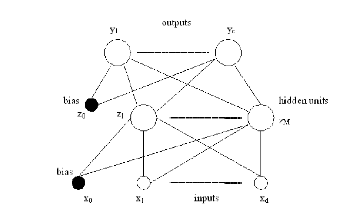
Note, however, that an alternative convention is sometimes also found in literature which counts layers of units rather than layers of weights, and regards the input as separate units. According to this convention the network showed in Fig. 1 would be called three-layer network. However, since the layers of adaptive weights are those which really matter in determining the properties of the network function, we refer to the former convention.
3.1 MLP: the flux of the computation
The MLP realizes a complex nonlinear mapping from the input to the output space. Let us denote the input values to the network by . The first layer of the network forms a linear combinations of these inputs to give a set of intermediate activation variables
| (1) |
with one variable associated with each of the hidden units. Here represents the elements of the first-layer weight matrix and are the biases parameters associated with the hidden units. The variables are then transformed by the nonlinear activation functions of the hidden layer. Here we restrict attention to activation functions. The outputs of the hidden units are then given by
| (2) |
The are then transformed by the second layer of weights and biases to give the second-layer activation values
| (3) |
where is the number of output units. Finally, these values are passed through the output-unit activation function to give output values , where . Depending on the nature of the problem under consideration we have:
-
•
for regression problems: a linear activation function, i.e. ;
-
•
for classification problems: a logistic sigmoidal activation functions applied to each of the output independently, i.e.:
3.2 MLP Training Phase
The basic learning algorithm for MLPs is the so called backpropagation and is based on the error-correction learning rule. In essence, backpropagation consists of two passes through the different layers of the network: a forward pass and a backward pass. In the forward pass an input vector is applied to the input nodes of the network, and its effect propagates through the network layer by layer. Finally, a set of outputs is produced as the actual response of the network. During the backward pass, on the other hand, the weights are all adjusted in accordance with the error-correction rule. Specifically, the actual response of the network is subtracted from a desired (target) response (which we denote as a vector ) to produce an error signal. This error signal is then propagated backward through the network. There are several choices for the form of the error signal to produce and this choice still depends on the nature of the problem, in particular:
-
•
for regression problems we adopted the sum-of-squares error function:
-
•
for classification problems we used the cross-entropy error function:
The weights are adjusted to make the actual response of the network move closer to the desired response in a statistical sense. In this work we adopted a computational more efficient variant of the backpropagation algorithm, namely the quasi-newton method. Furthermore, we employed a weight-decay regularization technique in order to limit the effect of the overfitting of the neural model to the training data, therefore the form of the error function is:
where the sum runs over all the weight and biases. The controls the extents to which the penalty term influences the form of the solution.
It must be stressed that the universal approximation theorem (Haykin, 1999) states that the two layers architecture is capable of universal approximation and a considerable number of papers have appeared in the literature discussing this property (cf. Bishop (1995) and reference therein). An important corollary of this result is that, in the context of a classification problem, networks with sigmoidal nonlinearities and two layer of weights can approximate any decision boundary to arbitrary accuracy. Thus, such networks also provide universal non-linear discriminant functions. More generally, the capability of such networks to approximate general smooth functions allows them to model posterior probabilities of class membership. Since two layers of weights suffice to implement any arbitrary function, one would need special problem conditions (Duda et al., 1973) or requirements to recommend the use of more than two layers. Furthermore, it is found empirically that networks with multiple hidden layers are more prone to getting caught in undesirable local minima. Astronomical data do not seem to require such level of complexity and therefore it is enough to use just a double weights layer, i.e a single hidden layer.
As it was just mentioned, it is also possible to train NNs in a Bayesian framework, which allows to find the more efficient among a population of NNs differing in the hyperparameters controlling the learning of the network (Bishop, 1995), in the number of hidden nodes, etc. The most important hyperparameters being the so called and . is related to the weights of the network and allows to estimate the relative importance of the different inputs and the selection of the input parameters which are more relevant to a given task (Automatic Relevance Determination; Bishop (1995)). In fact, a larger value for a component of implies a less meaningful corresponding weight. is instead related to the variance of the noise (a smaller value corresponding to a larger value of the noise) and therefore to a lower reliability of the network. The implementation of a Bayesian framework requires several steps: initialization of weights and hyperparameters; training the network via a non linear optimization algorithm in order to minimize the total error function. Every few cycles of the algorithm, the hyperparameters are re-estimated and eventually the cycles are reiterated.
4 The data and the ’base of knowledge’
The Sloan Digital Sky Survey (hereafter SDSS) is an ongoing survey to image approximately sterad of the sky in five photometric bands and it is also the only survey so far to be complemented by spectroscopic data for objects (cf. the SDSS webpages at http://www.sdss.org/ for further details). The existence of such spectroscopic subset (hereafter SpS), together with the accurate characterization of biases and errors renders the SDSS an unique and ideal playing ground on which to train and test most photometric redshifts methods.
Several criteria may be adopted in extracting galaxy data from the SDSS database (Yasuda et al., 2001). We preferred, however, to adopt the standard SDSS criterium and use the GALAXY table membership. The data used in this work were therefore extracted from the SDSS catalogues. More in particular, the spectroscopic subsample (hereafter SpS), used for training and testing purposes, was extracted from the Data Release 4 (hereafter DR4; cf. Adelman-McCarthy et al. (2006)) . While this work was in progress the Data Release 5 (DR5) was made publicly available. Thus, the photometric data used to produce the final catalogues were derived from the latter data. We wish to stress that this extension of the dataset was made possible by the fact that the properties of the DR5 are the same of the DR4 except for a wider sky coverage.
In this paper we made use of two different bases of knowledge extracted from the SpS of the DR4:
-
•
The General Galaxy Sample or GG: composed of objects with matching the following selection criteria: dereddened magnitude in band, ; which corresponds to primary objects only in the case of deblended sources.
-
•
The Luminous Red Galaxies sample or LRG: composed of red luminous galaxies candidates having spectroscopic redshift .
The SDSS spectroscopic survey (Eisenstein et al., 2001) was planned in order to favour the observation of the so called Red Luminous Galaxies or LRGs which are expected to represent a more homogeneous population of luminous elliptical galaxies which can be effectively used to trace the large scale structures (Eisenstein et al., 2001). We therefore extracted from the SDSS-DR4 all objects matching the above listed criteria and, furthermore, flagged as .
LRGs are of high cosmological relevance since they are both very luminous (and therefore allow to map the universe out to large distances), and clearly related to the cosmic structures (being preferably found in clusters). Furthermore, their spectral energy distribution is rather uniform, with a strong break at Å produced by the superposition of a large number of metal lines (Schneider et al., 1983; Eisenstein et al., 2003). LRGs are therefore an ideal target to test the validity of photometric redshift algorithms (see for instance: Hamilton (1985), Gladders & Yee (2000), Eisenstein et al. (2001), Willis et al. (2001) and Padmanabhan et al. (2005)). The selection of LRG objects was performed using the same criteria extensively described in Padmanabhan et al. (2005) and, given the rather lengthy procedure, we refer to that paper for a detailed description of the cuts introduced in the parameter space.
Since it is well known that photometric redshift estimates depend on the morphological type, age, metallicity, dust, etc. it has to be expected that if some morphological parameters are taken into account besides than magnitudes or colors alone, estimates of photometric redshifts should become more accurate. Such an effect was for instance found by Tagliaferri et al. (2002); Vanzella et al. (2004).
In order to be conservative and also because it is not always simple to understand which parameters might carry relevant information, for each object we extracted from the SDSS database not only the photometric data but also the additional parameters listed in Table 1.
These parameters are of two types: those which we call ’features’ (marked as in Table 1), are parameters which potentially may carry some useful information capable to improve the accuracy of photometric redshifts, while those named ’labels’ (marked as ) can be used to better understand the biases and the characteristics of the ’base of knowledge’.
For what magnitudes are concerned, and at a difference with other groups who used the , we used the so called dereddened magnitudes (dered), corrected for the best available estimate of the SDSS photometric zero-points:
as reported in Padmanabhan et al. (2005). It has to be stressed, however that such corrections are of little relevance for empirical methods since they affect equally all data sets.
| N | Parameter | F/L | |
|---|---|---|---|
| objID | SDSS identification code | – | |
| ra | right ascention (J2000) | – | |
| dec | declination (J2000) | – | |
| 1 | petroR50i | 50 of Petr. rad. in the -th band, | F |
| 2 | petroR90i | 90 of Petr. rad. in the -th band, | F |
| 3 | deredi | dered. mag. in the band, | F |
| 4 | lnLDeVr | log likelihood for De Vaucouleurs profile, r band | F |
| 5 | lnLExpr | log likelihood for exponential profile, r band | F |
| 6 | lnLStarr | log likelihood for PSF profile, r band | F |
| spectroscopic redshift | L | ||
| specClass | spectral classification index | L |
Note. — Column 1: running number for features only. Column 2: SDSS code. Column 3: short explanation. Column 4: type of parameter, either feature (F) or label (L).
Finally we must stress that we impose the condition that the objects had to be ’primary’ () and detected in all five bands. The latter condition being required by the fact that all empirical methods suffer, one way or the other, from the presence of missing data and, to our knowledge, no clear cut method has been found to overcome this problem.
4.1 Features selection
In order to evaluate the significance of the additional features, our first set of experiments was performed along the same line as described in Tagliaferri et al. (2002) using a Multi Layer Perceptron with 1 hidden layer and 24 neurons. In each experiment, the training, validation and test sets were constructed by randomly extracting from the overall dataset three subsets, respectively containing 60%, 20% and 20% of the total amount of galaxies.
On the sample, we run a total of experiments. The first one was performed using all features, while the other were performed taking away the feature with . For each experiment, following Csabai et al. (2003), we used the test set to evaluate the robust variance obtained by excluding all points whose dispersion is larger then 3 (see § 7). The values are listed in Table 2.
| Parameters | |
|---|---|
| all | 0.0202 |
| all but 1 | 0.0209 |
| all but 2 | 0.0213 |
| all but 4 & 5 | 0.214 |
| all but 6 | 0.215 |
| only magnitudes | 0.0199 |
Note. — Column 1: features used. Features are numbered as in Table 1. Column 2: robust sigma of the residuals.
As it can be seen, the most significant parameters are the magnitudes (or the colors). Other parameters affect only the third digit of the robust sigma and, due to the large increase in computing time during the training phase (which scales as , where is the number of input features) and to avoid loss of generality of higher redshifts, where additional features such as the Petrosian radii are either impossible to measure or affected by large errors, we preferred to drop all additional features and use only the magnitudes. The fact that on the contrary of what was found in Vanzella et al. (2004) and Tagliaferri et al. (2002) additional features do not play a significant role may be understood as a consequence of the fact that in this work the training set is much larger and more complete than in these earlier works and therefore the color parameter space is (on average, but see below) better mapped.
5 The evaluation of photometric redshifts
One preliminary consideration: as it was first pointed out by Connolly et al. (1995), when working in the near and intermediate redshift universe (), the most relevant broad band features are the Balmer break at Å and the shape of the continuum in the near UV. Near IR bands become relevant only at higher redshift and this is the main reason why we decided to concentrate on the near universe (), where the SDSS optical bands provide enough spectral coverage.
One additional reason comes from the redshift distribution of the objects in the SpS-DR4 shown in Fig. 2 (solid line). As it can be clearly seen, the histogram presents a clear discontinuity at ( of the objects have and only are at a higher redshift) and in practice no objects are present for .

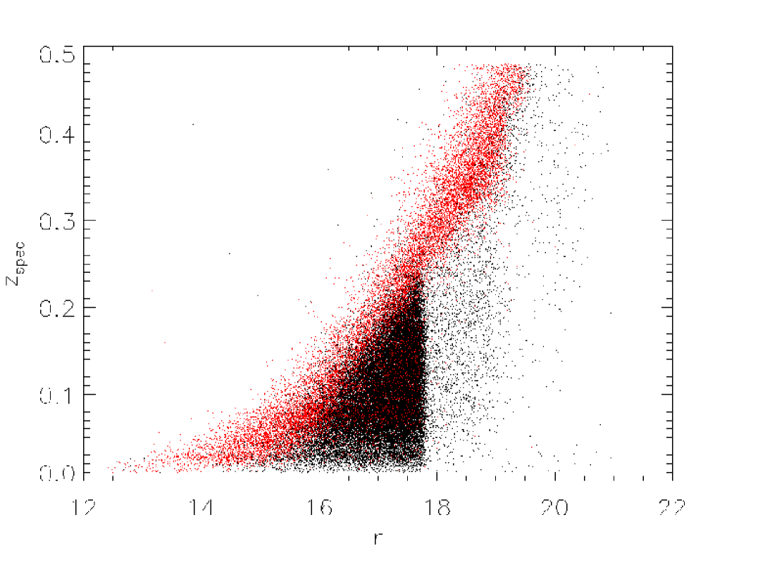
In Fig. 2 we also plot as dotted line the redshift distribution of the galaxies in the SpS data set which match the LRG photometric selection criteria. As it can be seen, within the tail at only a very small fraction (11.4%) of the objects does not match the LRG selection criteria. In Fig. 3 we plot the redshift of objects belonging to the GG sample against their luminosity in band: red dots represent those galaxies which have been a posteriori identified as LRG. As it is clearly seen, the overall distribution at redshift drops dramatically at , due to the selection criteria of the spectroscopic SDSS survey. At higher redshift, namely , the galaxy distribution is dominated by LRGs with few contaminants and extends to much fainter luminosities. Nevertheless LRGs are systematically brighter then GG galaxies all over the redshift interval .
Such large dishomogeneity in the density and nature of training data, poses severe constraints on any empirical method since the different weights of samples extracted in the different redshift bins would lead either to over fitting in the densest region, or to the opposite effect in the less populated ones. Furthermore, the dominance of LRGs at implies that in this redshift range the base of knowledge offers a poor coverage of the parameter space.
The first problem can be solved by taking into account the fact that, as shown in Tagliaferri et al. (2002); Firth et al. (2003) NNs work properly even with scarcely populated training sets, and by building a training set which uniformly samples the parameter space or, in other words, which equally weights different clusters of points (notice that in this paper we use the word cluster in the statistical sense, id est to denote a statistically significant aggregation of points in the parameter space). In the present case the dominance of LRGs at high redshifts renders the parameter space heavily undersampled.
In fact, as it will be shown in Paper III (D’Abrusco et al., 2006), a more detailed analysis of the parameter space shows that at high redshift, the objects group into one very large structure containing more than 90 of the data points, plus several dozens of much smaller clusters .
5.1 The nearby and intermediate redshifts samples
In order to tackle the above mentioned problems, we adopted a two steps approach: first we trained a network to recognize nearby (id est with ) and distant () objects, then we trained two separate networks to work in the two different redshift regimes. This approach ensures that the NNs achieve a good generalization capabilities in the nearby sample and leaves the biases mainly in the distant one. To perform the separation between nearby and distant objects, we extracted from the SDSS-4 SpS training, validation and test sets weighting, respectively, , and of the total number of objects (449,370 galaxies). The resulting test set, therefore, consisted of 89,874 randomly extracted objects. Extensive testing (each experiment was done performing a separate random extraction of training, validation and test sets) on the network architecture lead to a MLP with 18 neurons in 1 hidden layer. This NN achieved the best performances after 110 epochs and the results are detailed, in the form of a confusion matrix, in Table 3.
As it can be seen, this first NN is capable to separate the two classes of objects with an efficiency of , with slightly better performances in the nearby sample () and slightly worse in the distant one ().
| SDSS nearby | SDSS far | |
|---|---|---|
| NN nearby | 76498 | 1096 |
| NN far | 1135 | 11145 |
In Fig. 4 we plot against the redshift the percentage (calculated binning over the redshifts) for the objects in the test set which were misclassified (id est objects belonging to the nearby sample which were erroneously attributed to the distant one and viceversa). The distribution appears fairly constant from to , while higher (but still negligible respect to the total number of objects in the sample) percentages are found at the extremes.

Notice that, when using photometric data alone, the absence of training data for , does not allow to evaluate the fraction of contaminants having which are erroneously attributed to the distant sample. However, given the adopted cuts in magnitude, this number may be safely assumed to be negligible.
5.2 The photometric redshifts
Once the first network has separated the nearby and distant objects, we can proceed to the derivation of the photometric redshifts working separately in the two regimes. Since NNs are excellent at interpolating data but very poor in extrapolating them, in order to minimize the systematic errors at the extremes of the training redshift ranges we adopted the following procedure.
For the nearby sample we trained the network using objects with spectroscopic redshift in the range and then considered the results to be reliable in the range . In the distant sample, instead, we trained the network over the range and then considered the results to be reliable in the range .
In order to select the optimal NN architecture, extensive testing was made varying the network parameters and for each test the training, validation and test sets were randomly extracted from the SpS. The results of the Bayesian learning of the NNs were found to depend on the number of neurons in the hidden layer; for the GG (LRG) sample the performances were best when this parameter was set to 24 for the nearby sample and for the distant one (24 and 25 respectively for the LRG sample). In Fig. 5 we give the trends as a function of the number of hidden neurons, of the interquartile errors and robust dispersion obtained for the nearby and distant GG samples respectively.


For the GG sample, the best experiment, the robust variance turned out to be over the whole redshift range and and for the nearby and distant objects, respectively. For what the LRG sample is concerned, we obtained over the whole range, and and for the nearby and distant samples, respectively. In the upper panels of Figs. 6 and 7 we plot the spectroscopic versus the photometric redshifts for the GG and the LRG samples, respectively. Due to the huge number of points which would make difficult to see the trends in the densest regions, we preferred to plot the data using isocontours (using a step of 0.02 times the maximum data point density).
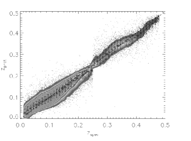
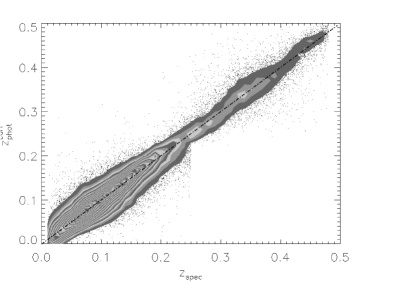
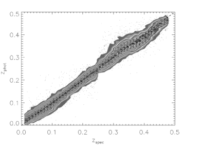
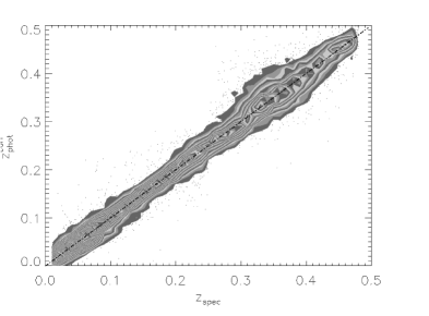
The mean value of the residuals are and for the GG and the LRG samples, respectively. These figures alone, however, are not very significant since systematic trends are clearly present in the data as it is shown in Fig. 8 and in Fig. 9, where we plot for each redshift bin the average value of the photometric redshifts and the robust sigma of the residuals.


6 Interpolative correction
The most significant deviations, as it could be expected (Connolly et al., 1995), are clearly visible in the nearby sample for and in the distant sample at . The first feature is due to the fact that at low redshifts faint and nearby galaxies cannot be easily disentangled by luminous and more distant objects having the same color. The second one is instead due to a degeneracy in the SDSS photometric system introduced by a small gap between the and bands. At , the Balmer break falls into this gap and its position becomes ill defined (Padmanabhan et al., 2005).
It needs to be stressed, however, that these trends represent a rather normal behavior for empirical methods which has already been explicitly noted in Tagliaferri et al. (2002) and Vanzella et al. (2004) and is clearly visible (even when it is not explicitly mentioned) in almost all photometric redshifts data sets (Wadadekar, 2005) available so far for the SDSS.
In order to minimize the effects of such systematic trends, but at the risk of a slight increase in the variance of the final catalogues we applied to both data sets an interpolative correction computed separatedly in the two redshift intervals. We used a ( fitting) to find, separately in each redshift regime, the polynomials which best fit the average points. These polynomials (of the fourth and fifth order, respectively) turned out to be. For the GG sample:
| (4) | |||||
| (5) |
and for the LRG sample:
| (6) | |||||
| (7) |
Thus, the correction to be applied is:
| (8) |
where for near objects and for the distant ones.
Obviously, when applying this method to objects for which we do not possess any spectroscopic estimate of redshift, it is impossible to perform the transformation (Eq. 8) to correct NNs estimates for systematic trends and we are obliged to use an approximation. In other words, we replace the unknown with in the Eq. (8), obtaining the relation:
| (9) |
where or depending on the redshift range.
This is equivalent to assuming that the same NNs distribution represents, with good approximation, the underlying and unknown distribution. After this correction we obtain a robust variance for the GG sample and for the LRG samples, computed in both cases over the whole redshift range, and the resulting distributions for the two samples are shown in the lower panels of Figs. 6 and 7.
7 Discussion of the systematics and of the errors
As noticed by several authors (see for instance, Schneider et al. (2006); Padmanabhan et al. (2005)), while some tolerance can be accepted on the amplitude of the redshift error, much more critical are the uncertainties about the probability distribution of those errors. This aspect is crucial since (Padmanabhan et al., 2005) the observed redshift distribution is related to the true redshift distribution via a Fredholm equation which is ill defined and strongly dependent on the accuracy with which the noise can be modeled. In this respect, many recent studies on the impact of redshift uncertainties on various cosmological aspects are available: dark energy from supernovae studies and cluster number counts (Huterer et al., 2004); weak lensing (Bernstein & Jain, 2004; Huterer et al., 2006; Ishak, 2005; Ma et al., 2006); baryon oscillations (Zhan, 2006; Zhan & Knox, 2006). All these studies model the error distribution as Gaussian.
However, photometric redshift error distributions, due to spectral-type/redshift degeneracies, often have bimodal distributions, with one smaller peak separated from a larger peak by z of order unity (Benítez, 2000; Fernández-Soto et al., 2001, 2002), or more complex error distributions, as it can be seen in Fig. 8 within the GG sample.
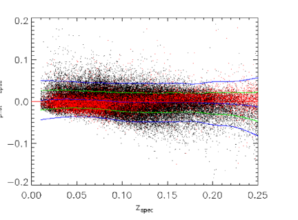
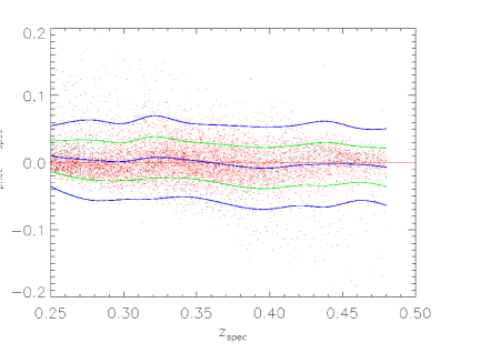
In order to evaluate the robustness of the , several instances of the process were applied to different randomly selected training, validation and test sets and the robust sigma was found to vary only on the fourth significant digit. Small differences were found only in the identification of catastrophic objects, which however did not present any significant variation in their frequency.
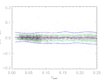
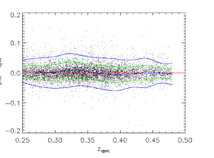
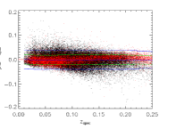
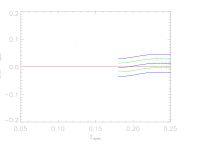
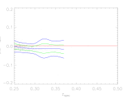
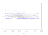
The distribution of the residuals as a function of the spectroscopic redshift for the GG and LRG samples is shown in Fig. 10 separately for the near and distant objects. We have also studied the dependance of such residuals from the -band luminosity of the galaxies in the two different magnitude ranges (cf. 5), ( and ) and in the near and intermediate redshift bins, as shown in Fig. 12 and Fig. 13 for the GG and LRG galaxies respectively. Clear systematics are found only for near/faint and intermediate/luminous LRGs residuals: in the former case, the mean value of residual is systematically higher then 0, while in the latter it is costantly biased to negative values. Both cases can be addressed reminding that these galaxies occupy a poorly sampled volume in the parameter-space, and therefore the NN fails to reproduce the exact trend of spectroscopic redshift.
In Fig. 11 we show the same plot as in Fig. 6 but without isocontours and plotting as red dots the objects which ”a posteriori” were labeled as members of the LRG sample. Interestingly enough, in the nearby sample the non-LRG and the LRG have robust variances of and . Notice, however, that the LRG objects show a clear residual systematic trend. This behaviour can be explained by the fact that in the nearby sample the training set contains a large enough number of examples for both samples of objects and the network can therefore achieve a good generalization capability. In the distant sample the Non-LRG and LRG objects have instead robust variances given by: and . Also in this case the observed behavior can be easily explained as due to the heavy bias toward the LRGs which form of the sample. It must be stressed that while the remaining of the objects still constitute a fairly large sample of objects, the uneven distribution of the training data between the two groups of objects, overtrains the NN toward the LRG objects which therefore are much better traced.
This confirms what already found by several authors (Padmanabhan et al., 2005): the derivation of photometric redshifts requires besides than an accurate evaluation of the errors also the identification of an homogeneous sample of objects.
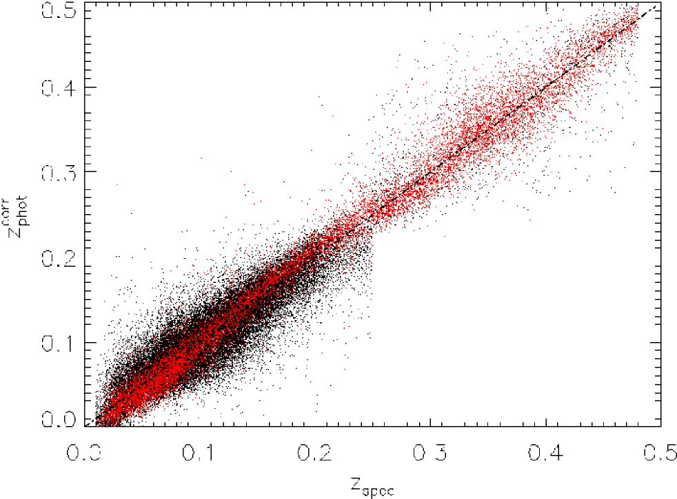
Objects not matching the criterium used for the robust variance are: 3.47 for the LRG sample and for the GG sample. Before correction, the rejected points are of the overall distribution for the GG sample and for the LRG one.
As it was already mentioned, the SDSS data set has been extensively analyzed by several authors who have used different methods for photometric redshift determination. Unfortunately, a direct comparison is not always possible due to differences in either the data sets (different data releases have been used) or in the way errors were estimated. It must be stressed, however, that due to the fact that, above a minimum and reasonably low treshold, the NN performances are not affected much by the number of objects in the training set, the former factor can be safely neglected. So far, the most extensive works are those by (Csabai et al., 2003) and Way & Srivastava (2006). In the former various methods were tested against the EDR data. With reference to their Table 3, and using the ’iterated’ which almost coincides with the robust variance adopted here, we find that the best performances were obtained, among the SED fitting methods for the BC synthetic spectra ( and , for the GG and LRG samples respectively. This method, however leads to very clear systematic trends and to a large number of catastrophic outliers (). Much better performances were attained by empirical methods and, in particular, by the interpolative one which leads to a ) with a fraction of catastrophic redshifts of only . In Way & Srivastava (2006) the authors made use of an Ensemble of NN (E) and Gaussian Process Regressions (GP). Their best results using the magnitudes only were and for the E and GP methods respectively, and at a difference with our method, their methods greatly benefits by the use of additional parameters such as the Petrosian radii, the concentration index and the shape parameter.
Two points are worth to be stressed. First of all, their selection criteria for the construction of the training set appear much more restrictive and it is not clear what performances could be achieved should such restriction be relaxed. Second, even though such ’ensemble’ approach is very promising and is likely to be the most general one, it has to be stressed that the bagging procedure, used in Way & Srivastava (2006) to combine the NNs, is known to be very effective only in those cases where the intrinsic variance of the adopted machine learning model is high. In this specific case, large number of training data and few input features, the NN result very stable and therefore other combining procedures, such as AdaBoost (Freund et al. (2003)), should be preferred (Dietterich (2002)). This might also be the reason why when only the photometric parameters are used their method gives slightly worse performances than ours and instead leads to better results when the number of features is increased.
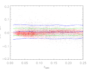
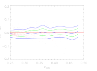
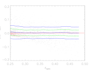
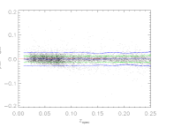
An additional machine learning approach, namely Support Vector Machines, was used by Wadadekar (2005). In Table 4 we shortly summarize the main results of the above quoted papers.

7.1 Contamination by distant galaxies
The fact that our NN’s are trained on a sample of galaxies with observed redshift introduces some contamination from objects which even though at still have and therefore match the photometric selection criteria.
The only possible way to avoid such an effect would be to use a knowledge base covering in an uniform way all significant regions of the photometric parameter space down to the adopted magnitude limit. In the case of SDSS this is true for magnitudes brighter than 17.7 but is not true at fainter light levels where the only region uniformously covered by the spectroscopic subsample is that defined by the LRG selection criteria. A possible way out could be to extend the base of knowledge to fainter light level by including stastically significant and complete samples of spectroscopic redshifts from other and deeper surveys. The feasibility of using a third NN to classify (and eventually throw into a waste basket) objects having is under study. At the moment, however, since we are interested in validating the method and in producing catalogues to be used for statistical applications, we shall estimate the number and the distribution in magnitude of such contaminants on statistical grounds only using the -band luminosity function derived from SDSS data by Blanton et al. (2003). This function, in fact, allows to derive for any given absolute magnitude the number of objects which even though at a redshift larger than 0.5 still match our apparent magnitude threshold and thus are misclassified. By integrating over the absolute magnitude and over the volume covered by the survey we obtain the curve in Fig. 14 which corresponds to a total number of contaminants of . It has to be noticed however that for magnitudes brighter than 20.5, the fraction of contaminants is less than and drops below for .
| Reference | Method | Data | Range | ||
|---|---|---|---|---|---|
| Csabai et al. (2003) | SED fitting CWW | EDR | 0.0621 | ||
| Csabai et al. (2003) | SED fitting BC | EDR | 0.0509 | ||
| Csabai et al. (2003) | interpolative | EDR | 0.0451 | ||
| Csabai et al. (2003) | bayesian | EDR | 0.0402 | ||
| Csabai et al. (2003) | empirical, polynomial fit | EDR | 0.0318 | ||
| Csabai et al. (2003) | K-D tree | EDR | 0.0254 | ||
| Suchkov et al. (2005) | Class X | DR-2 | 0.0340 | ||
| Way & Srivastava (2006)a | Gaussian Process | DR-3 | 0.0230 | ||
| Way & Srivastava (2006)a | ensemble | DR-3 | 0.0205 | ||
| Collister & Lahav (2004) | ANNz | EDR | 0.0229 | ||
| Wadadekar (2005) | SVM | DR-2 | 0.027 | ||
| Wadadekar (2005)a | SVM | DR-2 | 0.024 | ||
| Vanzella et al. (2004) | MLP ff | DR1 | 0.016 | 0.022 | |
| Padmanabhan et al. (2005) | Template fitting and Hybrid | DR1-LRG | |||
| this work before int. | MLP | DR5-GG | -0.0036 | 0.0197 | 0.01,0.25 |
| this work before int. | MLP | DR5-GG | -0.0036 | 0.0245 | 0.25,0.48 |
| this work after int. | MLP | DR5-GG | 0.01,0.25 | ||
| this work after int. | MLP | DR5-GG | 0.25,0.48 | ||
| this work before int. | MLP | DR5-LRG | -0.0029 | 0.0194 | 0.01,0.25 |
| this work before int. | MLP | DR5-LRG | -0.0029 | 0.0205 | 0.25,0.48 |
Note. — Column 1: reference; Column 2: method (for the acronyms see text); Column 3: data set (EDR=Early Data Release; DR1 through DR5 the various SDSS data release); Column 4: systematic offset; Column 5: standard deviation; Column 6: redshift range over which the average error is estimated.
(a): additional morphological and photometric parameters.
8 The catalogues
As mentioned above, the catalogues containing the photometric redshift parameters together with the parameters used for their derivation can be downloaded at the URL: . This data, for consistency with the SDSS survey, has been subdivided in several files, each corresponding to a different SDSS stripe of the observed sky. A stripe is defined by a line of constant survey latitude , bounded on the north and south by the edges of the two strips (scans along a constant value), and bounded on the east and west by lines of constant lambda. Because both strips and stripes are defined in ”observed” space, they are rectangular areas which overlap as one approaches the poles (for more details see ). The data for both GG and LRG samples have been extracted using the queries described in 4. The catalogues can be downloaded as ’FITS’ files, containing the fundamental parameters used for redshift determination and the estimated photometric redshift for each individual source. In more details (in brackets SDSS database names of the parameters): unique SDSS identifier (’objID’),right ascension J2000 (’ra’) declination J2000 (’dec’), dereddened magnitudes (’dered_u’, ’dered_g’, ’dered_r’, ’dered_i’, ’dered_z’), radius containing 50 of Petrosian flux for each magnitude (’petroR50_u’, ’petroR50_g’, ’petroR50_r’, ’petroR50_i’, ’petroR50_z’), radius containing 90 of Petrosian flux for each magnitude (’petroR90_u’, ’petroR90_g’, ’petroR90_r’, ’petroR90_i’, ’petroR90_z’), De Vaucouleurs fit ln(likelihood) in u and r bands (’lnLDeV_u’, ’lnLDeV_r’), exponential disc fit ln(likelihood) in u and r bands (’lnLExp_u’, ’lnLExp_r’).
9 Conclusions
In the previous paragraphs we discussed a ’two steps’ application of neural networks to the evaluation of photometric redshifts. Even though finely tailored on the characteristic of the SDSS, the method is completely general and can be easily applied to any other multiband data set provided that a suitable base of spectroscopic knowledge is available. As most other neural networks methods, several advantages are evident:
-
1.
The NN can be easily re-trained if new data become available. Even thoug the training phase can be rather demanding in terms of computing time, once the NN has been trained, the derivation of redshifts is almost immediate ( objects are processed on the fly on a normal laptop).
-
2.
Even though it was not necessary in this specific case, all sorts of a priori knowledge can be taken into account.
On the other end, the method suffers of those limitations which are typical of all empirical methods based on interpolation. Most of all, the training set needs to ensure a complete and if possible uniform coverage of the parameter space.
Our method allowed to derive photometric redshifts for with robust variances of for the GG sample ( and for the nearby and distant sample respectively) and for the LRG sample ( and ). This accuracy was reached adopting using a two-step approach allowing to build training sets which uniformly sample the parameter space of the overall population.
In the case of LRGs, the better accuracy and the close Gaussianity of the residuals, are explained by the fact that this sample was selected based on the a priori assumption that they form a rather homogeneous population sharing the same SED. In other words, this result confirms what has long been known, id est the fact that when using empirical methods, it is crucial to define photometrically homogeneous populations of objects.
In the more general case it would be necessary to define photometrically homogeneous populations of objects in absence of a priori information and therefore relying only on the photometric data themselves. This task, as it has been shown for instance by Suchkov et al. (2005); Bazell & Miller (2004) is a non trivial one, since the complexity of astronomical data and the level of degeneration is so high that most unsupervised clustering methods partition the photometric parameter space in far too many clusters, thus preventing the build-up a of a suitable base of knowledge. A possible way to solve this problem will be discussed in Paper III.
References
- Adelman-McCarthy et al. (2006) Adelman-McCarthy, J.K., et al. 2006, ApJS, 162, 38
- Ball et al. (2004) Ball, N. M., Loveday, J., Fukugita, M., Nakamura, O., Okamura, S., Brinkmann, J., & Brunner, R. J. 2004, MNRAS, 348, 1038
- Baum (1962) Baum, W. A. 1962, IAU Symp. 15: Problems of Extra-Galactic Research, 15, 390
- Bazell & Miller (2004) Bazell D., Miller D.J., astro-ph/0406323
- Bishop (1995) Bishop C.M., 1995, Neural Networks for Pattern Recognition, Oxford University Press
- Benítez (2000) Benítez, N. 2000, ApJ, 536, 571
- Bernstein & Jain (2004) Bernstein, G., & Jain, B. 2004, ApJ, 600, 17
- Blake & Bridle (2005) Blake, C., & Bridle, S. 2005, MNRAS, 363, 1329
- Blanton et al. (2003) Blanton, M.R., Hogg, D.W., Bahcall, N.A., Brinkmann, J., Britton, M., Connolly, A.J., Csabai, I., et al., 2003, ApJ, 592,819
- Bolzonella et al. (2000) Bolzonella, M., Miralles, J.-M., & Pelló, R. 2000, A&A, 363, 476
- Bolzonella et al. (2002) Bolzonella, M., Pelló R. & Maccagni D. 200, A&A, 395, 443
- Brescia et al. (2006) Brescia, M., De Filippis, E., D’Abrusco, R., Longo, G., Paolillo, M., & Staiano, A. 2006, in preparation
- Brodwin et al. (2006) Brodwin, M., Brown, M. J. I., Ashby, M. L. N., Bian, C., Brandt, K., Dey, A., Eisenhardt, P. R., Eisenstain, D. J., Gonzales, A. H., Huang, J. S., Jannuzi, B. T., Kochanek, C. S., McKenzie, E., Pahre, M. A., Smith, H. A., Soifer, B. T., Stanford, S. A., Stern, D., & Elston, R.J. 2006, astro-ph/0607450
- Brunner et al. (1999) Brunner, R. J., Connolly, A. J., & Szalay, A. S. 1999, ApJ, 516, 563
- Bruzual A. & Charlot (1993) Bruzual A., G., & Charlot, S. 1993, ApJ, 405, 538
- (16) Butchins, S. A. 1981, A&A, 97, 407
- Budavári et al. (2003) Budavári, T., et al. 2003, ApJ, 595, 59
- Collister & Lahav (2004) Collister, A. A., & Lahav, O. 2004, PASP, 116, 345
- Coleman et al. (1980) Coleman, G.D., Wu., C.-C., & Weedman, D.W., 1980, ApJS, 43, 393
- Connolly et al. (1995) Connolly, A. J., Csabai, I., Szalay, A. S., Koo, D. C., Kron, R. G., & Munn, J. A. 1995, AJ, 110, 2655
- Csabai et al. (2003) Csabai, I., et al. 2003, AJ, 125, 580
- D’Abrusco et al. (2006) D’Abrusco, R., Staiano, A., Longo, G., Brescia, M., De Filippis, E., Paolillo, M., & Tagliaferri, R. 2006, in preparation
- Dietterich (2002) Dietterich, T. G. 2002, in The Handbook of Brain Theory and Neural Networks, Second edition, M.A. Arbib ed., Cambridge, MA: The MIT Press, 405
- Donalek (2007) Donalek C., 2007, Ph.D. Thesis University of Napoli- Federico II
- Duda et al. (1973) Duda, R. O., Hart, P. E., & Stork, D. G. 2001, A Wiley-Interscience Publication, New York: Wiley, 2001
- Edmonson et al. (2003) Edmondson E.M., Miller L. & Wolf C. astro-ph/0607302
- Eisenstein et al. (2001) Eisenstein, D. J., et al. 2001, AJ, 122, 2267
- Eisenstein et al. (2003) Eisenstein, D. J., et al. 2003, ApJ, 585, 694
- Fernández-Soto et al. (2001) Fernández-Soto, A., Lanzetta, K. M., Chen, H.-W., Pascarelle, S. M., & Yahata, N. 2001, ApJs, 135, 41
- Fernández-Soto et al. (2002) Fernández-Soto, A., Lanzetta, K. M., Chen, H.-W., Levine, B., & Yahata, N. 2002, MNRAS, 330, 889
- Firth et al. (2003) Firth, A. E., Lahav, O., & Somerville, R. S. 2003, MNRAS, 339, 1195
- Freund et al. (2003) Freund, Y, Shapire R. E., 1996, Experiments with a new boosting algorithm, in Proc. 13th International Conferenze on Machine Learning.
- Gladders & Yee (2000) Gladders, M. D., & Yee, H. K. C. 2000, AJ, 120, 2148
- Hamilton (1985) Hamilton, D. 1985, ApJ, 297, 371
- Haykin (1999) Haykin, S., 1999, Neural Networks - A comprehensive Foundation, Second Edition, Prentice Hall
- Huterer et al. (2004) Huterer, D., Kim, A., Krauss, L. M., & Broderick, T. 2004, ApJ, 615, 595
- Huterer et al. (2006) Huterer, D., Takada, M., Bernstein, G., & Jain, B. 2006, MNRAS, 366, 101
- Ishak (2005) Ishak, M. 2005, MNRAS, 363, 469
- Koo (1999) Koo, D. C. 1999, ASP Conf. Ser. 191: Photometric Redshifts and the Detection of High Redshift Galaxies, 191, 3
- Ma et al. (2006) Ma, Z., Hu, W., & Huterer, D. 2006, ApJ, 636, 21
- Massarotti et al. (2001) Massarotti, M., Iovino, A., Buzzoni, A., & Valls-Gabaud, D. 2001, A&A, 380, 425
- Massarotti et al. (2001) Massarotti, M., Iovino, A., & Buzzoni, A. 2001, A&A, 368, 74
- Mobasher et al. (2004) Mobasher, B., et al. 2004, ApJl, 600, L167
- Padmanabhan et al. (2005) Padmanabhan, N., et al. 2005, MNRAS, 359, 237
- Puschell et al. (1982) Puschell, J. J., Owen, F. N., & Laing, R. A. 1982, ApJl, 257, L57
- Schneider et al. (1983) Schneider, D. P., Gunn, J. E., & Hoessel, J. G. 1983, ApJ, 264, 337
- Schneider et al. (2006) Schneider, M., Knox, L., Zhan, H. & Connolly, A. 2006, astro-ph/060698
- Suchkov et al. (2005) Suchkov A.A., Hanish R.J., Margon B., astro-ph/0508501
- Tagliaferri et al. (2002) Tagliaferri, R. et al. 2002, astro-ph/0203445
- Tagliaferri et al. (2003a) Tagliaferri, R., Longo, G., Milano, L., Acernese, F., Barone, F., Ciaramella, A., De Rosa, R., Donalek, C., Eleuteri, A., Raiconi, G., Sessa, S., Staiano, A., & Volpicelli, A. 2003, in the Special Issue on Neural Network Analysis of Complex Scientific Data: Astronomy and Geosciences, Neural Networks, 16, p 297
- Tagliaferri et al. (2003b) Tagliaferri, R., Longo, G., Andreon, S., Capozziello, S., Donalek, C., & Giordano, G. 2003, Lectures Notes in Computer Science, 2859, 226
- Tegmark et al. (2006) Tegmark, M. et al., 2006, astro-ph/0608632
- Wadadekar (2005) Wadadekar, Y. 2005, PASP, 117, 79
- Wang et al. (1998) Wang, Y., Bahcall, N., & Turner, E. L. 1998, AJ, 116, 2081
- Way & Srivastava (2006) Way, M. J., & Srivastava, A. N. 2006, ApJ, 647, 102
- Yasuda et al. (2001) Yasuda, N., et al. 2001, AJ, 122, 1104
- Yip et al. (2004) Yip, C. W., et al. 2004, AJ, 128, 585
- Vanzella et al. (2004) Vanzella, E., et al. 2004, A&A, 423, 761
- Willis et al. (2001) Willis, J. P., Hewett, P. C., & Warren, S. J. 2001, MNRAS, 325, 1002
- Winter et al. (2004) Winter, C. Jeffery, C.S., Drilling, J.S., 2004, ApSS, 291, 375
- Zhan & Knox (2006) Zhan, H., & Knox, L. 2006, ApJ, 644, 663
- Zhan (2006) Zhan, H. 2006, Journal of Cosmology and Astro-Particle Physics, 8, 8