AO assisted spectroscopy with SINFONI: PSF, background, and interpolation

I discuss 3 widely applicable aspects concerning calibration of the near infrared adaptive optics integral field spectrometer SINFONI: (1) the accuracy with which one needs to quantify the PSF and how this might be achieved in practice; (2) how it is possible to fine tune the background subtraction to minimise the residual OH airglow; and (3) how an altered perspective on calibration data might lead to improvements in interpolation and greater flexibility in reconstructing datacubes.

1 A Short Introduction to SINFONI

SINFONI davies:eis03a ; davies:bon04 is a versatile instrument comprising of a 60-element curvature adaptive optics system davies:bon03 that feeds a 1–2.5 $\mu$m integral field spectrometer davies:eis03b . The camera has 3 pixel scales spanning 0.25^′′ to 0.025^′′, making it adaptable to both seeing and diffraction limited and resolutions. The associated fields of view range from $8^{\prime\prime}\times 8^{\prime\prime}$ to $1^{\prime\prime}\times 1^{\prime\prime}$. It can cover the H and K bands together in a single exposure at a spectral resolution of $R\sim 1500$; or a complete single waveband (J, H, or K) at $R\sim 2000$–5000, depending on the pixel scale. Since the highest resolution (associated with the smallest pixel scale) is under-sampled, one has the option of spectrally dithering and interleaving the 2 exposures. Image slicers dissect the field of view and re-arrange the slitlets along a single pseudo-slit. On the detector, the dispersed data from each slitlet appear exactly analogous to standard longslit data, except that there are 32 such 2D spectra next to each other. A dedicated data reduction package spred davies:abu05 reconstructs the 3D datacube. An excellent tool for viewing them is QFitsView (see http://www.mpe.mpg.de/~ott/QFitsView), which displays the spectrum in real time as one moves the pointer across the spatial field. With this tool it is also extremely quick and simple to apply a wide range of processing techniques in real time.

2 The Adaptive Optics Point Spread Function

Misunderstandings about adaptive optics PSF abound: that it must be known in great detail, and that its temporal and spatial variability casts doubt on interpretation of the data. In this section, I attempt to alleviate these concerns by discussing some ideas about the level of accuracy with which one needs to know the PSF, and some ways in which this might be achieved.

2.1 Quantifying the PSF

There will always be some situations where it is necessary to know the PSF in great detail, most obviously in planet searches where one is trying to detect small faint object close around a bright point source. In these cases, it is crucial to distinguish between the object and structure that belongs to the PSF. On the other hand, many – perhaps most – applications do not require such a detailed level of knowledge. Particularly for extragalactic science, where the AO correction is mediocre, a simple combination of 2 analytical functions will often suffice. For example, the PSF can be generally well matched by the sum of a narrow Gaussian, which represents the core of the PSF, and a Moffat function which can trace the wide wings in the halo. Greater detail in the PSF is unnecessary because the accuracy is limited by the model (kinematic or morphological), which, in contrast to the real intrinsic structure in galaxies, is usually simple, and often symmetric.

2.2 (De)-convolution

Figure 1: Velocity and dispersion fields for matter in a self-gravitating disk around a supermassive black hole. In the field shown, the integrated mass of the disk is 5 times that of the black hole. The effect of PSF-induced smearing on the kinematics is very dramatic. Due to cross-talk between these 2 quantities (i.e. velocity gradients on scales comparable to the PSF contribute to the dispersion), the smeared kinematics cannot be deconvolved. The only option is to create a 3D kinematic model (2 spatial and 1 velocity dimension), convolve it with the PSF, and then extract the kinematics. By iterating one can constrain the model parameters.

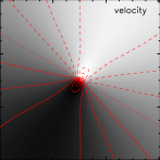
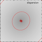
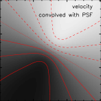
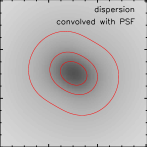
Dealing with a PSF that comprises 2 contrasting components – a narrow core and broad wings – is an important issue. Clearly one needs to separate the PSF from the instrinsic structure in the observed data. But deconvolution is not always the best solution. It is an inverse problem, and hence mathematically messy, tends to amplify noise, and can easily generate unreal artifacts (e.g. ringing). And at the end, one still has no convenient expression for the intrinsic source shape and one still has to deal with a PSF in the deconvolved data. It may be narrower, but it is probably less well defined and may vary with signal-to-noise across the field. In some cases, such as kinematics (Fig. 1), deconvolution is simply not an option due to the cross-talk between the velocity and dispersion.

Figure 2: Example of a faint $K_{s}=19.2$ galaxy observed with adaptive optics davies:cre05 . The galaxy was 18.3” from the guide star, and so the PSF derived for it had to take into account isoplanatic effects (see point (iii) below). The image of the galaxy (left) is too noisy to deconvolve with the PSF. It has therefore been fitted by convolving the PSF with a parameterised galaxy profile (centre). The parameters of the profile were adjusted to minimise the residuals (right). This can yield not only the best fitting parameters, but also a good estimate of their uncertainties.

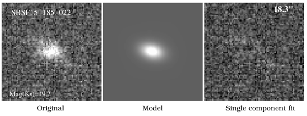
An alternative is to convolve a model of the intrinsic structure with the PSF, compare the result to the observations, and adjust the model iteratively. This is the basis of popular galaxy fitting algorithms, such as galfit davies:pen02 which has been used in Fig. 2. The method also enables one to make realistic estimates of the uncertainty in the fitted parameters. While it cannot be used if there is no way to parameterise the instrinsic source structure (e.g. the features on the surface of a planet such as Titan), it is still widely applicable.

2.3 Methods to estimate the PSF

Below are suggested several ways one might try to infer the shape of the PSF. This list is not necessarily exhaustive, but is intended to indicate that many possibilities exist if one can be a little inventive.

(i) Reconstruct it from the wavefront sensor data
From the astronomer’s perspective, this is the ideal option. PSF reconstruction has been developed for both curvature davies:ver97 and Shack-hartmann AO systems davies:wei03 ; davies:jol04 , and there are no technical limitations. However, there is no general facility for PSF reconstruction yet available at the VLT. A tool is being developed for NACO (see Clenet’s contribution to this proceedings).

(ii) Use an isolated star as a reference
This is generally the path recommended to an observer. However, for practical reasons – specifically the time needed to slew to and observe a separate reference star – it is often impractical. Furthermore, a reliable PSF estimate requires that the intensity and distribution of flux on the WFS is the same for the reference star as for the science wavefront reference object. 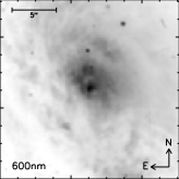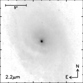If both are stars, this can work well; but as Fig 3 shows for AGN and other extended sources, it is simply unreliable.

Figure 3: Images of the Circinus galaxy: left optical, right near infrared davies:pri04 . It is impossible to reproduce the flux distribution seen by a visible WFS using a reference star. On the other hand, what an infrared WFS sees is dominated by a point source and so it may be possibleto use a reference star to estimate the PSF.

To complicate the matter further, if the wavefront reference is not the science target, then using it to estimate the PSF is misleading due to anisoplanaticism. Instead one needs to find a pair of stars (e.g. from the Washington Double Star Catalog davies:mas01 ) separated by the same distance, one of which matches the guide star magnitude and the other of which can be observed by the science camera.

(iii) Extrapolate it from surrounding stars
If one is lucky, it may be possible to measure the PSF from nearby stars davies:pri04 . More often, it will be necessary to account for anisoplanaticism. Several methods have been developed to estimate an off-axis PSF; and in principle these could be turned around to derive an on-axis PSF from off-axis stars. Typically, they require knowledge of the $C_{N}^{2}$ distribution through the atmosphere davies:fus00 ; davies:bri06 or observations of calibration frames containing many stars davies:ste02 . But it is also possible to make a reasonable (and sufficient) approximation to the way the PSF varies across a wider field using the science data alone, as long as at least one or two stars or compact objects are detected davies:cre05 ; davies:cre06 .

(iv) Extract it from the science data itself
The broad line region in AGN is only a few lightdays across and is therefore always unresolved in 8-m class telescopes. In addition, the near-infrared non-stellar continuum associated with AGN is only 1–2 pc across and hence unresolved in AGN that are at least $\sim 20$ Mpc away. The spatial distribution of both these quantities can be extracted using the spectral information available in a near infrared datacube, and has been used as an estimate of the PSF in several cases davies:dav04a ; davies:dav04b ; davies:dav06 .

One might expect that it should also be possible to extract information about the PSF from other science data in an analogous way.

(v) Derive it by comparison to other higher resolution data
If data taken with another instrument at another time exist at the same wavelength and at higher spatial resolution, one might derive the PSF by reference to these davies:mul06 . This is because convolution of the PSF $P$ with the intrinsic source $S$ yields the observed source $O=P\otimes S$. One can define a broadening function $F$ which, when convolved with the higher resolution observation $O_{h}$, reproduces the lower resolution observation $O_{l}=O_{h}\otimes F$. Then by definition the lower resolution PSF is $P_{l}=P_{h}\otimes F$.

2.4 Effects of LGS adaptive optics

The VLT Laser Guide Star Facility has recently been commissioned, and so the observer will soon have to cope with LGS-AO data. Because the wavefront reference will be the same regardless of the science target, the PSF should in principle be easier to measure using an isolated reference stars as in point (ii) above. In addition, because the LGS samples a cone rather than a full column through the atmosphere, the isoplanatic effects will be smaller. The main impact on the PSF will be residual jitter from the tip-tilt star, which depends on how faint and how far away it is. But this is relatively easy to add in afterwards to an initial (better) estimate of the PSF.

3 Improving the Background Subtraction

Figure 4: Noise in sky subtracted H-band SINFONI cubes (arbitrary data units) for consecutive 5 min integrations. Pluses denote cubes which each had a different sky cube, taken immediately afterwards, subtracted. Diamonds show the resulting noise level when this was performed using the scaling algorithm described in the text.

A method to improve subtraction of the near infrared background, which is dominated by OH emission lines, has recently been described davies:dav07 . This is based on the fact that most of the variation between these lines occurs from changes in the vibrational rather than rotational temperature of the OH radical. And grouping the emission lines according to the vibrational part of their transition can be done to a reasonable approximation by wavelength: any particular spectral segment contains all the strong lines for one specific vibrational transition. One can then apply an appropriate scaling to the sky frame for each segment separately before subtracting it. Since the segments span a reasonably wide wavelength range, the method is robust against emission or absorption features being blended with OH lines. Treatment of the rotational part of the transitions is similar, although trickier because they cannot be grouped so easily and also because OH lines from different transitions are blended. The integration of this background subtraction algorithm into the SINFONI pipeline is described by Modigliani in this proceedings.

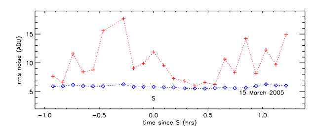
A quantitative indication of the improvement this method can yield is given in Fig. 4. In this experiment, a long sequence of blank 5 min H-band SINFONI frames were used. For each frame, the successive one was used to subtract the sky background. The noise in the sky-subtracted cube – which is dominated by residual OH emission – was measured as the standard deviation of all data values within the spatial field and spanning 1.55-1.75 $\mu$m. The figure shows that the noise is variable and high. Using this new algorithm not only reduced the residual noise by the resulting noise is much more stable across all the frames. In fact, this method allows one to use fewer sky frames, thus significantly increasing the observing efficiency.

One aspect that also needs to be addressed in relation to background subtraction is the accuracy of the wavelength calibration. It is a feature of SINFONI data that there may be a shift of a fraction of a pixel along the spectral axis between frames. If this is not corrected, then subtracting a sky frame will leave P-Cygni residuals for the OH lines. This can be corrected by reconstructing each cube before subtracting the background, measuring the wavelength of each strong OH line, and deriving the mean spectral offset. The whole frame can then be shifted by an appropriate amount to correct the offset. Details of all these aspects are described elsewhere davies:dav07 .

4 Interpolating in 3 Dimensions

Figure 5: Illustrative example of an alternative perspective for reconstructing datacubes. (a) observed data are sampled regularly in the reference frame of the detector. (b) this sampling is irregular in the reference frame of the reconstructed cube; bad pixels can simply be omitted from the set of sampled points. (c) one can freely specify the required gridding (i.e. spatial/spectral pixel scale) for the reconstructed data; it is independent of the actual sampling. (d) each required grid point is interpolated from sampled points which lie in its local neighbourhood. Any suitable algorithm can be used for the interpolation.

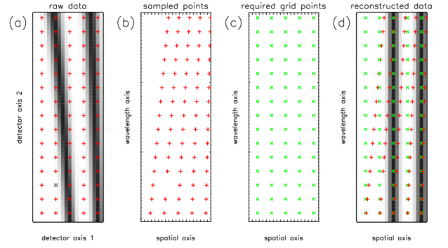
Interpolation is a crucial issue for integral field spectroscopy, since reconstructing 3D datacubes requires a significant amount of interpolation. In the classical approach, one needs to correct for bad pixels, straighten the spectral traces, linearise the dispersion, and finally align the slitlets (or pixels). Tuning the wavelength scale to correct for flexures between frames (as described in Section 3) can introduce an additional interpolation step. Poor management of the interpolation strategy or poor choice of the interpolation scheme can degrade the quality of the final data. For this reason, I propose an alternative perspective on the purpose of calibrations which allows one to view the data reconstruction in a different way – enabling one to perform all the interpolation in a single step while at the same time permitting a far greater flexibility. This can be summarised as follows:

Standard View
calibrations allow one to create the mathematical functions necessary (e.g. polynomials) to correct the spectral and spatial curvature on the detector.

Alternative View
calibrations allow one to create look-up tables which associate each measured value on the detector with its spectral and spatial location in the final reconstructed data.

This new perspective, which is incorporated into the design of the KMOS data reduction library, is outlined graphically in Fig. 5. The most important realisation is that in ‘detector space’ there can be no concept of a wavelength or spatial axis. These concepts apply only to the final reconstructed cube. The detector is nothing more than the medium on which raw data values are recorded. The calibrations allow one to assign each measured value on the detector to a spatial/spectral location in the reconstructed cube. Together, these locations provide an irregularly spaced sampling of that cube. Ihe aim is thus to reduce the raw data and the calibrations to a list of values with their associated locations:

$$\begin{array}[]{cccc}value_{0},&x_{0},&y_{0},&\lambda_{0}\\ value_{1},&x_{1},&y_{1},&\lambda_{1}\\ \vdots&\vdots&\vdots&\vdots\\ value_{n},&x_{n},&y_{n},&\lambda_{n}\\ \end{array}$$

Data associated with bad pixels is simply excluded from the list and so does not contribute to the set of sampled locations. Creation of this list is the first step. The second step is to specify the regular sampling – i.e. the spatial and spectral pixel size – that is required for the reconstructed cube. The third step is to interpolate each of these regularly gridded positions from sampled locations in the local neighbourhood. In a fourth step, one can determine any spectral (or spatial) offsets in the reconstructed cube and feed these back to create a new list with updated locations for each measured value. One can then re-interpolate the regular grid of points, leading to a final cube which has been reconstructed in a single interpolation and which has no offsets. There are a number of advantages of this method:

• Only a single interpolation is required to reconstruct the final cube from the raw data. This leads to improved noise properties in the final cube.

• One can combine separate frames during this interpolation, by concatenating their lists of data values and locations. This is useful because it avoids the need to shift and combine cubes afterwards.

• One has a free choice of spatial and spectral sampling in the final cube. This is useful if one wants to compare the data to that from another instrument: one can reconstruct the cube at the appropriate pixel scale, rather than having to re-interpolate it afterwards.

• One has the option of smoothing the data during the reconstruction. If the data is particularly noisy, one can increase the size of the local neighbourhood around each point to reduce the noise at the expense of resolution.

References

- (1) Abuter R., et al.: NewAR, 50, 398 (2005)
- (2) Bonnet H., et al.: SPIE, 4839, 329 (2003)
- (3) Bonnet H., et al.: ESO Messenger, 117, 17 (2004)
- (4) C. Britton: PASP, 118, 885 (2006)
- (5) G. Cresci, R. Davies, A. Baker, M. Lehnert: A&A, 438, 757 (2005)
- (6) G. Cresci, R. Davies, A. Baker, F. Manucci, M. Lehnert, T. Totani, Y. Minowa: A&A, 458, 385 (2006)
- (7) R. Davies, L. Tacconi, R. Genzel: ApJ, 602, 148 (2004)
- (8) R. Davies, L. Tacconi, R. Genzel: ApJ, 613, 781 (2004)
- (9) R. Davies, et al.: ApJ, 646, 754 (2006)
- (10) R. Davies: MNRAS, 375, 1099 (2007)
- (11) F. Eisenhauer et al.: ESO Messenger, 113, 17 (2003)
- (12) F. Eisenhauer et al.: SPIE, 4841, 1548 (2003)
- (13) T. Fusco, J.-M. Conan, L. Mugnier, V. Michau, G. Rousset: A&AS, 142, 149 (2000)
- (14) L. Jolissaint, J.-P. Véran, J. Marino: SPIE, 4590, 151 (2004)
- (15) B. Mason, G Wycoff, W Hartkopf, G Douglass, C Worley: AJ, 122, 3466 (2001)
- (16) F. Mueller Sánchez, R. Davies, F. Eisenhauer, L. Tacconi, R. Genzel, A. Sternberg: A&A, 454, 481 (2006)
- (17) C. Peng, L. Ho, C. Impey, H.-W. Rix: AJ, 124, 266 (2002)
- (18) A. Prieto, et al.: ApJ, 614, 135 (2004)
- (19) E. Steinbring et al.: PASP, 114, 1267 (2002)
- (20) J.-P. Véran, F. Rigaut, H. Maître, D. Rouan: JOSA, 14, 3057 (1997)
- (21) R. Weiss: PhD thesis, University of Heidleberg (2003)