Completeness I: revisited, reviewed and revived

Abstract

We have extended and improved the statistical test recently developed by Rauzy for assessing the completeness in apparent magnitude of magnitude-redshift surveys. Our improved test statistic retains the robust properties – specifically independence of the spatial distribution of galaxies within a survey – of the $T_{c}$ statistic introduced in Rauzy’s seminal paper, but now accounts for the presence of both a faint and bright apparent magnitude limit. We demonstrate that a failure to include a bright magnitude limit can significantly affect the performance of Rauzy’s $T_{c}$ statistic. Moreover, we have also introduced a new test statistic, $T_{v}$, defined in terms of the cumulative distance distribution of galaxies within a redshift survey. These test statistics represent powerful tools for identifying and characterising systematic errors in magnitude-redshift data.

We discuss the advantages of the $T_{c}$ and $T_{v}$ statistics over standard completeness tests, particularly the widely used $\cal{V}$/$\cal{V}$_max test which assumes spatial homogeneity, and we demonstrate how our $T_{v}$ statistic can essentially be regarded as an improved, cumulative $\cal{V}$/$\cal{V}$_max test which makes better use of the magnitude completeness information in a redshift survey. Finally we apply our completeness test to three major redshift surveys: The Millennium Galaxy Catalogue (MGC), The Two Degree Field Galaxy Redshift Survey (2dFGRS), and the Sloan Digital Sky Survey (SDSS). We confirm that MGC and SDSS are complete up to the published (faint) apparent magnitude limit of $m_{b_{j}}=20.00$ mag. and $m_{r}=17.45$ mag. respectively, indicating there are no residual systematic effects within the photometry. Furthermore, we show that, unless a bright limit is included for 2dFGRS, the data-set displays significant incompleteness at magnitudes brighter than the published limit of $m_{b_{j}}=19.45$ mag.

1 Introduction

In recent years the statistical analysis of galaxy redshift surveys has become a thriving industry in cosmology, yielding powerful constraints on the parameters of both the underlying cosmological world model and on the luminosity distribution of galaxies as a function of redshift, environment and morphological type. However, both tasks are rendered complicated by the presence of observational selection effects – due to e.g. detection thresholds in apparent magnitude, colour, surface brightness or some combination thereof. Over many years, therefore, a wide range of statistical tools has been developed to identify, characterise – and hopefully to remove – the impact of observational selection effects from magnitude-redshift surveys.

Of particular interest are data-sets which are complete in apparent magnitude – meaning that all galaxies brighter than some specified limiting apparent magnitude (or, as is pertinent to this paper, with apparent magnitudes lying between some specified bright and faint limiting values) have been observed. The case of magnitude-redshift data truncated by a faint apparent magnitude limit has been extensively discussed in the literature and well-established techniques have been developed for reconstructing the galaxy luminosity function in this case. These include, for example, the $C-$ method of Lynden-Bell (1971), the maximum likelihood fitting method of Sandage et al. (1979) and the stepwise maximum likelihood method of Efstathiou et al. (1988). However, these methods are formulated under the assumption that the survey data are complete in apparent magnitude; hence, the assumption of magnitude completeness must be rigourously checked.

A classical test for completeness in apparent magnitude is to analyse the variation in galaxy number counts as a function of the adopted limiting apparent magnitude (Hubble 1926). This test, which presupposes that the galaxy population does not evolve with time and is homogeneously distributed in space, is however not very efficient. More specifically, it is difficult to decide in practice whether deviations from the expected galaxy number count is indeed an effect of incompleteness in apparent magnitude, or is due to galaxy clustering and/or evolution of the galaxy luminosity function, or is indeed created by incompleteness in apparent magnitude. Of course in designing a completeness test one can also make use of distance information via galaxy redshifts; the well-known $\cal{V}$/$\cal{V}$_max test of Schmidt (1968) does this, and considers – for a specified magnitude limit – the ratio of two volumes: the volume of a sphere of radius equal to the actual distance of observed galaxy, divided by the volume of a sphere of radius equal to the maximum distance at which the galaxy would be observable – i.e. at the apparent magnitude limit. It follows that – for a non-evolving, homogeneous distribution of galaxies – the expected value of $\cal{V}$/$\cal{V}$_max is equal to $1/2$. The $\cal{V}$/$\cal{V}$_max test has been used to assess the completeness of magnitude-redshift samples (see for example Hudson and Lynden-Bell (1991), but unfortunately it suffers from the same major drawbacks as the Hubble test based on galaxy number counts: it is difficult to interpret whether any significant measured departure from the expected value of $\cal{V}$/$\cal{V}$_max is due to incompleteness or to clustering and evolutionary effects.

In an important (although rarely cited) paper, Efron and Petrosian (1992) introduced a powerful new approach to analysing magnitude-redshift surveys. They proposed a non-parametric test for the independence of the spatial and luminosity distributions of galaxies in a magnitude-limited sample, which required no assumptions concerning the parametric form of both the spatial distribution and the galaxy luminosity function. They applied this test to a quasar sample, with an assumed apparent magnitude limit, in order to robustly estimate the cosmological parameters characterising the luminosity distance-redshift relation of the quasars (see also (Efron and Petrosian, 1998)).

Rauzy (2001) noted that the essential ideas of Efron & Petrosian could be straightforwardly adapted and extended to turn their non-parametric test of the cosmological model into a non-parametric test of the assumption of a magnitude-limited sample – thus developing a simple but powerful tool for assessing the magnitude completeness of magnitude-redshift surveys. As was the case with Efron & Petrosian – and unlike the Hubble number counts or $\cal{V}$/$\cal{V}$_max tests – the Rauzy test statistic requires no assumption that the spatial distribution of galaxies is homogenous. Moreover, it also requires no knowledge of the parametric form of the galaxy luminosity function. On the other hand, the Rauzy test was formulated only for the case of a sharp, faint apparent magnitude limit. The aim of this paper will be to extend Rauzy’s formalism to account for a bright apparent magnitude limit, and to apply the extended completeness test to several recent galaxy redshift surveys.

This paper is, therefore, organised as follows. In Section 2 we review the completeness test introduced by Rauzy (2001) and extend it to the case of a galaxy survey with both a faint and a bright apparent magnitude limit. In Section 3 we then introduce a further variant on the original Rauzy completeness test, which is based on the cumulative distance distribution of observable galaxies in a magnitude-redshift survey. In Section 4 we briefly describe the properties of three recent redshift surveys: the Millennium Galaxy Catalogue, the Sloan Digital Sky Survey and the Two Degree Field Galaxy Redshift Survey. In Section 5 we then apply our new completeness test to these three surveys, investigating their completeness in apparent magnitude. Finally, in Section 6 we summarise our conclusions.

Figure 1: Schematic diagram illustrating the construction of the rectangular regions $S_{1}$ and $S_{2}$, defined for a typical galaxy at $(M_{i},Z_{i})$. The left panel shows the original R01 construction of regions $S_{1}$ and $S_{2}$. The right hand panel shows the construction of regions $S_{1}$ and $S_{2}$ with the inclusion of a bright limit. These regions are uniquely defined for a slice of fixed width, $\delta Z$, in corrected distance modulus, and for ‘trial’ bright and faint apparent magnitude limits $m^{\rm b}_{*}$ and $m^{\rm f}_{*}$ respectively. Also shown are the true bright and faint apparent magnitude limits $m^{\rm b}_{\rm lim}$ and $m^{\rm f}_{\rm lim}$, within which the rectangular regions $S_{1}$ and $S_{2}$ contain a joint distribution of $M$ and $Z$ that is separable.

2 Extending the Rauzy completeness test

In this section we review briefly the robust completeness test introduced by Rauzy (2001; hereafter R01) and applied in Rauzy et al. (2001), and extend it to include the effect of an imposed bright apparent magnitude limit to a magnitude-redshift survey. While this extension is straightforward, our approach in this paper will be rather pedagogical in order to benefit those readers not previously familiar with the formalism previously developed in R01 and Rauzy, Hendry & D’Mellow (2001).

2.1 Assumptions and statistical model

The fundamental assumption of the Rauzy completeness test is that the luminosity function of the galaxy population does not depend on the 3-D redshift space position $\mathbf{z}=(z,l,b)$ of the galaxies. Although this assumption is restrictive, note that it is common to most classical number counts tests of completeness and indeed (when applied in the context of assessing magnitude completeness) the $\cal{V}$/$\cal{V}$_max test. Moreover, the results derived in Appendix 1 of Rauzy, Hendry & D’Mellow (2001) imply that the completeness test of R01 remains valid in the case of pure density evolution. Note also that the completeness test remains valid for the case of pure luminosity evolution provided that an evolution correction is applied to account for the (assumed known) functional dependence of the mean luminosity at given redshift. For clarity, we will defer until a subsequent paper the interesting case where one wishes simultaneously to assess the magnitude completeness and estimate the parameters of a luminosity evolution model. In this paper, where appropriate, we will apply evolutionary and extinction corrections from the literature to the photometry of the galaxy surveys we consider. Specifically, following the notation of R01, we introduce the corrected distance modulus $Z$, defined as

$$Z=m-M=\mu(z)+k_{\rm cor}(z)+e_{\rm cor}(z)+A_{g}(l,b),$$ (1)

where $\mu(z)$ is the (cosmological model-dependent) distance modulus at redshift $z$, $k_{\rm cor}(z)$ and $e_{\rm cor}(z)$ are $k$-corrections and evolutionary corrections respectively and $A_{g}(l,b)$ is an extinction correction dependent on galactic co-ordinates $(l,b)$. Note, however, as will be seen in Section 5 below, that the application (or not) of $k$-corrections and evolutionary corrections generally does not have a strong impact on the performance of our completeness test. Neglecting for the moment any observational selection effects, the joint probability density in position and absolute magnitude for the galaxy population can be written as

$$d{P_{zM}}\ {\propto}\ d{P_{z}}\ \times\ {dP_{M}}\ =\ {\rho}(z,l,b)dldbdz\times f(M)dM,$$ (2)

where ${\rho}(z,l,b)$ is the 3D redshift space distribution function of the sources along the past light-cone and $f(M)$ is the galaxy luminosity function, defined following e.g. Binggeli et al. (1988). We now take as our null hypothesis that the selection effects are separable in position and apparent magnitude, and that the observed sample is complete in apparent magnitude for those objects which are simultaneously brighter than a specified faint apparent magnitude limit, $m^{\rm{f}}_{\rm{lim}}$, and fainter than a specified bright apparent magnitude limit, $m^{\rm{b}}_{\rm{lim}}$. Under this null hypothesis the selection function $\psi(m,z,l,b)$ can be written as

$$\psi(m,z,l,b)\equiv\theta(m^{\rm f}_{\rm lim}-m)\times\theta(m-m^{\rm b}_{\rm lim})\times\phi(z,l,b),$$ (3)

where $\theta(x)$ is the Heaviside or ‘step’ function defined as

$$\theta(x)=\left\{\begin{array}[]{ll}1&\quad{\rm if}\,\,x\geq 0,\\ 0&\quad{\rm if}\,\,x<0,\end{array}\right.$$ (4)

and $\phi(z,l,b)$ describes the selection effects in angular position and observed redshift. Taking into account this model for the selection effects, the probability density function describing the joint distribution of absolute magnitude $M$ and corrected distance modulus $Z$ for the observable galaxy population may therefore be written as

$$dP=\overline{h}(Z)dZ\,f(M)dM\,\theta(m^{\rm f}_{\rm lim}-m)\theta(m-m^{\rm b}_{\rm lim}),$$ (5)

where $\overline{h}(Z)$ is the probability density function of $Z$ for observable galaxies, marginalised over direction on the sky, i.e.

$$\overline{h}(Z)=\int_{l}\,\int_{b}\,h(Z,l,b)dldb,$$ (6)

and the integrand $h(Z,l,b)$ is equal to the (suitably normalised) product of the 3-D redshift space density $\rho(z,l,b)$ and the selection function $\phi(z,l,b)$, re-expressed as a function of $Z$.

Note from Equation (5) that the faint and bright apparent magnitude limits introduce a correlation between the variables $M$ and $Z$ for observable galaxies.

2.2 Defining the random variable $\zeta$

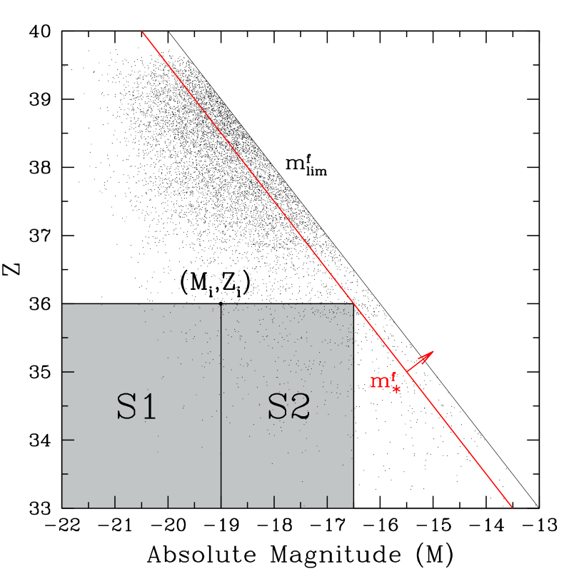
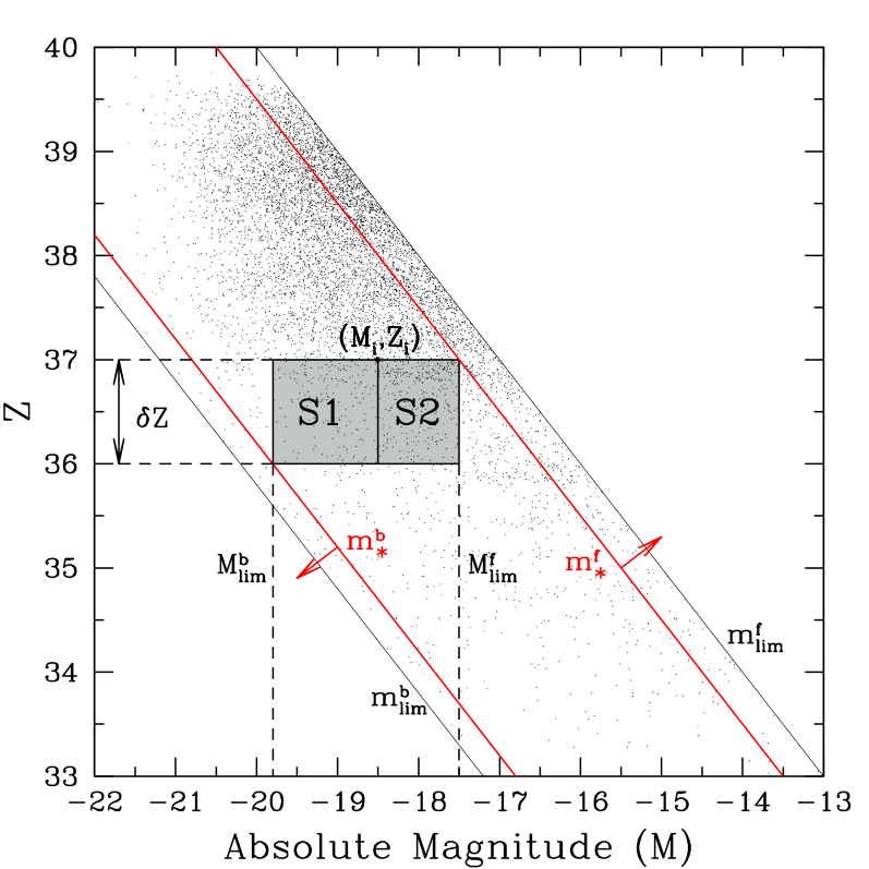
As in R01, the key element of our extended completeness test is the definition of a random variable, $\zeta$, related to the cumulative luminosity function of the galaxy population. We proceed in a similar manner to R01, but now with both a bright and faint apparent magnitude limit. To see how we construct $\zeta$ in this more general case consider Fig. 1, which schematically represents an $M-Z$ plot of corrected distance modulus versus absolute magnitude for the observable population of galaxies. The left hand panel shows this plot for the case of a faint apparent magnitude limit only, as was considered in R01. The right hand panel is for the more general case which we consider here. Shown on the right hand panel are solid diagonal lines representing the ‘true’ faint and bright apparent magnitude limits, $m^{\rm f}_{\rm{lim}}$ and $m^{\rm b}_{\rm{lim}}$ respectively, while the bold diagonal lines represent putative faint and bright magnitude limits, $m^{\rm f}_{*}$ and $m^{\rm b}_{*}$ respectively. The position $(M_{i},Z_{i})$ of the $i^{\rm{th}}$ galaxy is also indicated on both panels, and the schematic diagrams are superimposed on the actual $M-Z$ distribution for the Millennium Galaxy Catalogue (Driver et al. 2005; see below).

In graphical terms, the essential idea of our completeness test is to identify from the data the faintest value of $m^{\rm f}_{*}$ and the brightest value of $m^{\rm b}_{*}$ which together bound a rectangular region of the $M-Z$ plane, within which the joint distribution of $M$ and $Z$ for observable galaxies is separable. If we compare the left and right hand panels of Fig. 1, we can see that the addition of a bright magnitude limit has an important impact on the construction of this separable region: in short, the region is no longer unique. However, if we fix the width, $\delta Z$, in corrected distance modulus as shown in the right hand panel of Fig. 1, the corresponding separable region is now uniquely defined. Moreover we can then define for the $i^{\rm th}$ galaxy the following absolute magnitudes:

• $M^{\rm f}_{\rm lim}(Z_{i})$, the absolute magnitude of a galaxy, at corrected distance modulus $Z_{i}$, which would be observed at the true faint apparent magnitude limit $m^{\rm f}_{\rm lim}$,

• $M^{\rm b}_{\rm lim}(Z_{i}-\delta Z)$, the absolute magnitude of a galaxy, at corrected distance modulus $Z_{i}-\delta Z$, which would be observed at the true bright apparent magnitude limit $m^{\rm b}_{\rm lim}$.

These two absolute magnitudes are indicated, for the putative magnitude limits $m^{\rm f}_{*}$ and $m^{\rm b}_{*}$, by the vertical dashed lines in the right hand panel of Fig. 1.

We now define the random variable $\zeta$ as follows

$$\zeta=\frac{F(M)-F(M^{\rm b}_{\rm lim}(Z-\delta Z))}{F(M^{\rm f}_{\rm lim}(Z))-F(M^{\rm b}_{\rm lim}(Z-\delta Z))},$$ (7)

where $F(M)$ is the Cumulative luminosity function, i.e.

$$F(M)=\int_{-\infty}^{M}f(x)dx.$$ (8)

It is straightforward to show from this definition that the random variable $\zeta$ has a uniform distribution on the interval $[0,1]$, and furthermore that $\zeta$ and $Z$ are statistically independent. Thus $\zeta$ shares the same two defining properties as the corresponding random variable defined in R01. Equation (7) therefore generalises the definition of $\zeta$ to the case of a galaxy survey with bright and faint magnitude limits. The relevance of $\zeta$ as a diagnostic of magnitude completeness will be demonstrated in the next two sections.

2.3 Estimating $\zeta$ and computing the $T_{c}$ statistic

As was the case in R01, the random variable $\zeta$ has the very useful property that we can estimate it without any prior knowledge of the cumulative luminosity function $F(M)$. Given a value of $\delta Z$, it is clear from Fig. 1 that for each point $(M_{i},Z_{i})$ in the $M-Z$ plane we can define the regions $S_{1}$ and $S_{2}$ as follows:

• $S_{1}=\{(M,Z):M^{\rm b}_{\rm lim}\leq M\leq M_{i},\,\,Z_{i}-\delta Z\leq Z\leq Z_{i}\},$

• $S_{2}=\{(M,Z):M_{i}<M\leq M^{\rm f}_{\rm lim},\,\,Z_{i}-\delta Z\leq Z\leq Z_{i}\}.$

In the special case where there is no bright limit the regions $S_{1}$ and $S_{2}$ are as shown in the left hand panel of Fig. 1.

Clearly the random variables $M$ and $Z$ are now independent within each sub-sample $S_{1}$ and $S_{2}$. Therefore from Equation (5) the number of points $r_{i}$ belonging to $S_{1}$ satisfies

$$\frac{r_{i}}{N_{\rm gal}}=\int_{Z_{i}-\delta Z}^{Z_{i}}\overline{h}(Z^{\prime})dZ^{\prime}\,\times\,\int_{M^{\rm b}_{\rm lim}}^{M_{i}}f(M)\,dM,$$ (9)

where $N_{\rm gal}$ is the total number of galaxies in the sample. Similarly the number of points $n_{i}$ in $S_{i}=S_{1}\cup S_{2}$ satisfies

$$\frac{n_{i}}{N_{\rm gal}}=\int_{Z_{i}-\delta Z}^{Z_{i}}\overline{h}(Z^{\prime})dZ^{\prime}\,\times\,\int_{M^{\rm b}_{\rm lim}}^{M^{\rm f}_{\rm lim}}f(M)\,dM.$$ (10)

The integrals over absolute magnitude in Equations (9) and (10) may be rewritten as

$$\int_{M^{\rm b}_{\rm lim}}^{M_{i}}f(M)\,dM\,=\,F\left(M_{i}(Z_{i})\right)-F\left(M^{\rm b}_{\rm lim}(Z_{i})\right),$$ (11)

and

$$\int_{M^{\rm b}_{\rm lim}}^{M^{\rm f}_{\rm lim}}f(M)\,dM\,=\,F\left(M^{\rm f}_{\rm lim}(Z_{i})\right)-F\left(M^{\rm b}_{\rm lim}(Z_{i})\right).$$ (12)

Thus, given a pair of ‘trial’ magnitude limits $m^{\rm f}_{*}$ and $m^{\rm b}_{*}$, it follows from Equations (7) and (9) to (12) that an estimate of $\zeta$ for the $i^{\rm th}$ galaxy is simply the ratio of the number of galaxies belonging to $S_{1}$ and $S_{1}\cup S_{2}$ respectively (where $M^{\rm b}_{*}$ and $M^{\rm f}_{*}$ replace $M^{\rm b}_{\rm lim}$ and $M^{\rm f}_{\rm lim}$ in the definition of $S_{1}$ and $S_{2}$). In fact an unbiased estimate of $\zeta$ for the $i^{\rm th}$ galaxy is (c.f. R01)

$${\hat{\zeta}_{i}}=\frac{r_{i}}{n_{i}+1}.$$ (13)

This estimator is identical to that defined in R01; the introduction of a bright magnitude limit has simply changed the definition of the random variable $\zeta$ itself and the membership criteria of the two regions $S_{1}$ and $S_{2}$. Thus, provided that both $m^{\rm f}_{*}\leq m^{\rm f}_{\rm lim}$ and $m^{\rm b}_{*}\geq m^{\rm b}_{\rm lim}$, then under our null hypothesis ${\hat{\zeta}_{i}}$ will be uniformly distributed on $[0,1]$ and uncorrelated with $Z_{i}$, exactly as was the case in R01. Moreover the expectation value $E_{i}$ and the variance $V_{i}$ of the $\hat{\zeta}_{i}$ are given respectively by

$$E_{i}=E(\hat{\zeta}_{i})=\frac{1}{2},\quad V_{i}=E\left[\left(\hat{\zeta}_{i}-E_{i}\right)^{2}\right]=\frac{1}{12}\,\frac{n_{i}-1}{n_{i}+1}.$$ (14)

Note that $V_{i}$ tends towards the variance of a continuous uniform distribution between 0 and 1 when $n_{i}$ is large.

As in R01, we can, therefore, combine the estimator ${\hat{\zeta}_{i}}$ for each observed galaxy into a single statistic, $T_{c}$, which we can use to test the magnitude completeness of our sample for adopted trial magnitude limits $m^{\rm f}_{*}$ and $m^{\rm b}_{*}$. $T_{c}$ is defined as

$$T_{c}={\displaystyle\sum_{i=1}^{N_{\rm gal}}\left({\hat{\zeta}_{i}}-\frac{1}{2}\right)}\Bigg{/}{{\displaystyle\left(\sum_{i=1}^{N_{\rm gal}}V_{i}\right)^{\frac{1}{2}}}}.$$ (15)

If the sample is complete in apparent magnitude, for a given pair of trial magnitude limits, then $T_{c}$ should be normally distributed with mean zero and variance unity. If, on the other hand, the trial faint (bright) magnitude limit is fainter (brighter) than the true limit, $T_{c}$ will become systematically negative, due to the systematic departure of the $\hat{\zeta}_{i}$ distribution from uniform on the interval $[0,1]$.

3 $T_{v}$: A variant of the Rauzy completeness test

Figure 2: : Schematic diagram illustrating the construction of the rectangular regions $S_{3}$ and $S_{4}$, defined for a typical galaxy at $(M_{i},Z_{i})$, which feature in the estimation of our new completeness test statistic, $T_{v}$. Panel (a) illustrates how $S_{3}$ and $S_{4}$ are constructed for a survey with only a faint magnitude limit $m^{\rm f}_{\rm lim}$, and are shown for a trial faint limit $m^{\rm f}_{\star}$. Panel (b) illustrates the case where the survey also has a true bright limit $m^{\rm b}_{\rm lim}$, and the rectangles are constructed for trial bright and faint limits $m^{\rm b}_{\rm lim}$ and $m^{\rm f}_{\rm lim}$ respectively. Note that the construction of the rectangles is unique for a ‘slice’ of fixed width, $\delta M$, in absolute magnitude.

In Section 1 we remarked on the similarities between the $\cal{V}$/$\cal{V}$_max test statistic and the completeness test of R01. We now introduce a further variant on the test statistic $T_{c}$, related to the distribution of corrected distance modulus for observable galaxies in a magnitude-redshift survey.

3.1 Defining the random variable $\tau$

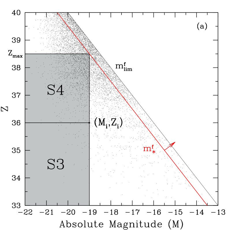
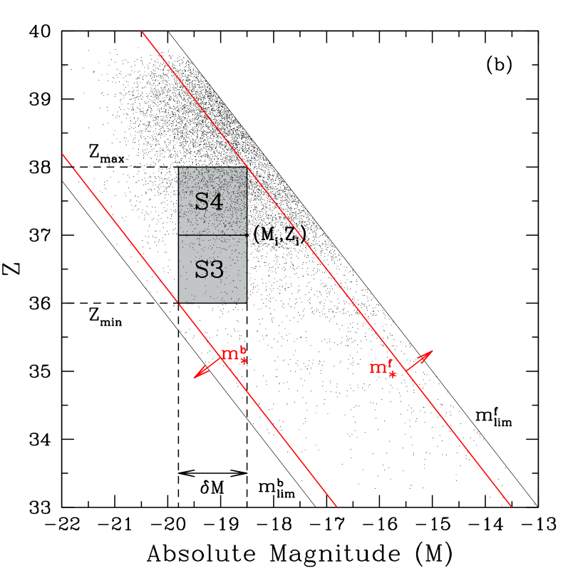
Fig.  2 shows schematic $M-Z$ plots, analogous to Fig. 1: the left panel again has a faint apparent magnitude limit only while the right hand has a ‘true’ bright and faint apparent magnitude limit, $m^{\rm b}_{\rm lim}$ and $m^{\rm f}_{\rm lim}$, with ‘putative’ bright and faint limits, $m^{\rm b}_{\rm*}$ and $m^{\rm f}_{\rm*}$ respectively, shown as the bold diagonal lines. Again, the position, $(M_{i},Z_{i})$, of a typical galaxy is shown on each panel, and the schematic plots are superimposed on the actual $M-Z$ distribution of the Millennium catalogue.

In the right hand panel of Fig.  2, however, we consider a ‘slice’ of width $\delta M$ in absolute magnitude brighter than $M_{i}$, as shown. We see that, given $m^{\rm b}_{\rm lim}$, $m^{\rm f}_{\rm lim}$ and $\delta M$, we can define for the $i^{\rm th}$ galaxy the following corrected distance moduli:

• $Z_{\rm upp}(M_{i})$, the corrected distance modulus of a galaxy, with absolute magnitude $M_{i}$, which would be observed at the true faint apparent magnitude limit $m^{\rm f}_{\rm lim}$,

• $Z_{\rm low}(M_{i}-\delta M)$, the corrected distance modulus of a galaxy, with absolute magnitude $M_{i}-\delta M$, which would be observed at the true bright apparent magnitude limit $m^{\rm b}_{\rm lim}$.

These two limiting distance moduli are indicated, for the putative magnitude limits $m^{\rm f}_{*}$ and $m^{\rm b}_{*}$, by the horizontal dashed lines in Fig.  2.

We now define a new random variable $\tau$ as follows. Let $H(Z)$ denote the cumulative distribution function of corrected distance modulus for observable galaxies, i.e.

$$H(Z)=\int_{-\infty}^{Z}\,\overline{h}(Z^{\prime})\,dZ^{\prime}.$$ (16)

Then $\tau$ is defined as

$$\tau=\frac{H(Z)-H(Z_{\rm low}(M-\delta M))}{H(Z_{\rm upp}(M))-H(Z_{\rm low}(M-\delta M))}.$$ (17)

As was the case for the random variable $\zeta$, it is straightforward to show that $\tau$ possesses the following properties:

• P1: $\tau$ is uniformly distributed between $0$ and $1$,

• P2: $\tau$ and $M$ are statistically independent.

These two properties are exactly analogous to the defining properties of $\zeta$, except that $\tau$ is now independent of corrected absolute magnitude, $M$. Once again we can use property P1 to construct a test for completeness in apparent magnitude.

3.2 Estimating $\tau$ and computing the $T_{v}$ statistic

Under the assumptions introduced in the previous section, it follows that $\tau$ can be estimated from our observed data without any prior knowledge of the spatial distribution of galaxies. To see how this estimate is constructed, consider again the right hand panel of Fig.  2. For each point with co-ordinates $(M_{i},Z_{i})$ in the $M-Z$ plane we can define the regions $S_{3}$ and $S_{4}$ as follows:

• $S_{3}=\{(M,Z):M_{i}-\delta M\leq M\leq M_{i},\,\,Z_{\rm low}\leq Z\leq Z_{i}\},$

• $S_{4}=\{(M,Z):M_{i}-\delta M\leq M\leq M_{i},\,\,Z_{i}\leq Z\leq Z^{i}_{\rm upp}\}.$

In the special case where there is no bright limit the regions $S_{3}$ and $S_{4}$ are as shown in the left hand panel of Fig. 1. Indeed, in this case, $S_{3}$ is identical to the region $S_{1}$ shown on the left hand panel of Fig. 2.

As was the case in Section 2, we see that the random variables $M$ and $Z$ are independent in each sub-sample $S_{3}$ and $S_{4}$. Therefore we can estimate $\tau$ by counting the number, $s_{i}$, of galaxies that belong to $S_{3}$ and the number, $t_{i}$, of galaxies that belong to $S_{3}\cup S_{4}$. As in Section 2, an unbiased estimate of $\tau$ is given by

$${\hat{\tau}_{i}}=\frac{r_{i}}{t_{i}+1}.$$ (18)

Thus, provided that both $m^{\rm f}_{*}\leq m^{\rm f}_{\rm lim}$ and $m^{\rm b}_{*}\geq m^{\rm b}_{\rm lim}$, then under our null hypothesis ${\hat{\tau}_{i}}$ will be uniformly distributed on $[0,1]$ and uncorrelated with $Z_{i}$, exactly as for $\hat{\zeta}_{i}$. Moreover the expectation $E_{i}$ and variance $V_{i}$ of the ${\hat{\tau}_{i}}$ are respectively

$$E_{i}=E(\hat{\tau}_{i})=\frac{1}{2},\quad V_{i}=E\left[\left(\hat{\tau}_{i}-E_{i}\right)^{2}\right]=\frac{1}{12}\,\frac{t_{i}-1}{t_{i}+1}.$$ (19)

Again, the variance of $\hat{\tau}_{i}$ tends towards that of a continuous uniform distribution between 0 and 1 for large $t_{i}$.

We can, therefore, again combine the estimator ${\hat{\tau}_{i}}$ for each observed galaxy into a single statistic, $T_{v}$, which we can use to test the magnitude completeness of our sample for adopted trial magnitude limits $m^{\rm f}_{*}$ and $m^{\rm b}_{*}$. $T_{c}$ is defined as

$$T_{v}={\displaystyle\sum_{i=1}^{N_{\rm gal}}\left({\hat{\tau}_{i}}-\frac{1}{2}\right)}\Bigg{/}{{\displaystyle\left(\sum_{i=1}^{N_{\rm gal}}V_{i}\right)^{\frac{1}{2}}}}.$$ (20)

If the sample is complete in apparent magnitude, for a given pair of trial magnitude limits, then $T_{v}$ should be normally distributed with mean zero and variance unity. If, on the other hand, the trial faint (bright) magnitude limit is fainter (brighter) than the true limit, in either case $T_{v}$ will become systematically negative, due to the systematic departure of the $\hat{\tau}_{i}$ distribution from uniform on the interval $[0,1]$.

4 THE DATA

We will now apply the tools developed in the previous section to test the magnitude completeness of three major redshift surveys: the Millennium Galaxy Catalogue (MGC), the Two Degree Field Galaxy Redshift Survey (2dFGRS) and The Sloan Digital Sky Survey (SDSS-DR1, Early Types). For ease of comparison we have assumed the same background cosmological model but have applied existing selection criteria (detailed below) for each survey.

4.1 Cosmology

Unless otherwise stated we have adopted throughout a ‘Concordance’ cosmology with present-day matter density $\Omega_{\rm m0}=0.3$ and cosmological constant term $\Omega_{\Lambda 0}$ = 0.7, and with a value of $H_{0}$ = 100 kms^-1 Mpc^-1 for the Hubble Constant throughout.

In order to convert the apparent magnitudes published for each survey to corrected absolute magnitudes we apply the following relation:

$$M_{i}=m_{i}-5\log_{10}(d_{L_{i}})-25-A_{g}(l,b)-k_{\rm cor}(z_{i})-e_{\rm cor}(z_{i}),$$ (21)

where $d_{L_{i}}$ is the luminosity distance (in Mpc) of the i^th galaxy given by:

$$d_{L_{i}}=(1+z_{i})\left(\frac{c}{H_{0}}\right)\int^{z_{i}}_{0}\frac{dz}{\sqrt{(1+z_{i})^{3}\Omega_{m0}+\Omega_{\Lambda 0}}},$$ (22)

and the other terms are as defined in Section 2.1 above.

4.2 Selection limits, $k$-corrections and evolutionary corrections

4.2.1 2dFGRS

The $2dF$ Galaxy Redshift Survey measured redshifts using the multifibre spectrograph on the Anglo-Australian Telescope. We have used the 2dFGRS public final release data-set, from the $`best\ observations^{\prime}$ spectroscopic catalogue, which records redshifts for a total of 245,591 sources.

The corresponding photometry was taken from the APM galaxy catalogue (Maddox et al. 1990) for galaxies brighter than an apparent magnitude of $m_{b_{j}}=19.45$ mag. The 2dFGRS survey region covered two strips: one $75^{\circ}\times 10^{\circ}$ around the north galactic pole and the other $80^{\circ}\times 15^{\circ}$ around the southern galactic pole.
To construct a clean catalogue, we firstly selected those galaxies with reliable redshifts – i.e all galaxies with a published redshift quality $Q_{z}\geq 3$. We then imposed maximum and minimum limits in redshift following Cross et al. 2001 – i.e. redshifts in the range $0.015<z<0.12$. From the parent catalogue of 245,591 sources we use a total of 111,082 galaxies.
There have been a variety of $k$-corrections and evolutionary corrections applied to the 2dFGRS. In our analysis we have adopted those applied by Cross (2001) and by Norberg (2002a, b).

4.2.2 The SDSS early-type galaxy sample

For our analysis we used galaxies selected from the Sloan Digital Sky Survey (SDSS) database. See Stoughton et al. (2002) for a description of the Early Data Release; Abazajian et al. (2003) et al. for a description of DR1, the First Data Release; Gunn et al. (1998) for a detailed description of the camera; Fukugita et al. (1996), Hogg et al. (2001) and Smith et al. (2002) for details of the photometric system and calibration; Lupton et al. (2001) for a discussion of the photometric data reduction pipeline; York et al. (2002) for a technical summary of the SDSS project; Pier et al. (2003) for the astrometric calibrations; Blanton et al. (2003) for details of the tilling algorithm; Strauss et al. (2002) and Eisenstein et al. (2001) for details of the target selection.
In broad terms, the SDSS sample includes spectroscopic information as well as photometric measurements in the $u^{*},g^{*},r^{*},i^{*}$ and $z^{*}$ bands. The SDSS First Data Release covers an area of $\approx$ 2000 deg² (Abazajian et al. 2003) on the sky.
The main quantities used in this work are the absolute and apparent magnitudes, and redshifts present in the SDSS-First Data Release, early types only (hereinafter referred to as ’SDSS-DR1’ ). The selection criteria has been discussed in Bernardi et al. (2003) and the data-set compiled in Bernardi et al. (2005). 39,320 objects have been targeted as early-type galaxies and having dereddened Petrosian (hereinafter referred to as, $m_{r}$) apparent magnitude (14.5 $<m_{r}<$ 17.75), and a redshift range of (0.0 $<z<$ 0.4). To calculate the distance modulus we assume a Hubble constant of 70 km s^-1 Mpc^-1.

4.2.3 The Millennium Galaxy Catalogue

The Millennium Galaxy Catalogue (MGC) is a medium-deep, $B_{j}$-band imaging survey, spanning 30.9 deg² that is fully contained within the 2dFGRS and SDSS-DR1. The full catalogue contains 10095 galaxies out to a published limiting apparent magnitude of $m_{b_{j}}=20.00$ mag (e.g. see Cross et al. (2004) for more detail). The photometry was obtained with the Wide Field Camera on the 2.5 m Isaac Newton Telescope in La Palma. The spectroscopy was constructed mainly from the redshifts obtained in the 2dFGRS and SDSS. In addition, the MGC team measured their own redshifts using the spectrograph on the Anglo-Australian Telescope for galaxies in the catalogue that had no assigned redshift.
Similarly with the 2dFGRS catalogue, only galaxies of a redshift quality $Q_{z}\geq 3$ have been selected. For ease of comparison we have imposed the same redshift cut as Driver et al. (2005) – i.e only galaxies in the range $0.013<z<0.18$ were included. From the parent catalogue of 10,095 galaxies this yields a sub set of 7,878 galaxies. Where appropriate we have applied the $k$-corrections and evolutionary corrections as described in detail by Driver et al. (2005).

5 Results

5.1 Testing the MGC dataset

5.1.1 The Rauzy method with a faint limit only

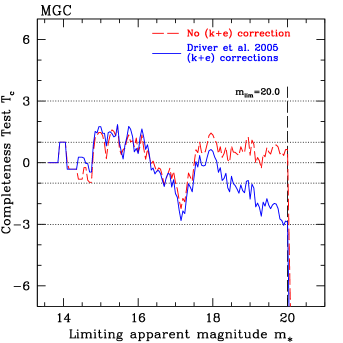
Fig. 3 shows the $T_{c}$ statistic as applied to the MGC survey. Since there was no bright limit published for this dataset we can use the traditional construction of the random variable $\zeta$ as described in R01. The dashed curve shows the $T_{c}$ statistic, as a function of trial magnitude limit, computed using apparent magnitudes that have not been $(k+e)$-corrected, but have been corrected for extinction only. The figure clearly shows that the $T_{c}$ statistic remains within the $3\sigma$ limits – consistent with being complete in apparent magnitude – up to the published magnitude limit of 20.0 mag., but then drops very sharply for trial apparent magnitude limits beyond 20.0 mag.
The solid curve on the same plot again shows the $T_{c}$ statistic as a function of trial magnitude limit but now computed for $(k+e)$-corrected apparent magnitudes. Although the MGC dataset is still consistent with being complete up to the published magnitude limit of 20.0 mag., there is a noticeable departure in the behaviour of $T_{c}$ from that for the uncorrected dataset: for trial magnitude limits in the range $m_{b_{j}}\approx 17.5$ to $m_{b_{j}}=20.00$, $T_{c}$ for the corrected dataset exhibits a slow decline, before again dropping sharply beyond 20.0 mag. The most likely explanation for this feature seems to lie in the way the dataset is selected and corrected. The raw dataset, with uncorrected magnitudes, has the same magnitude limit imposed on all galaxies independent of their galaxy type. If, then, each galaxy is individually $(k+e)$-corrected, the resultant overall magnitude limit for the corrected data will become ‘fuzzy’ without a sharp cut-off. Furthermore, different galaxy populations will be scattered differently, leading to a smooth decrease close to the original uncorrected magnitude limit. On the other hand, if we do not apply a $(k+e)$-correction, the original magnitude limit remains defined (albeit now without explicitly accounting for the effects of evolution and redshifting of each galaxy’s spectral energy distribution). Therefore, to obtain an improved measure of completeness which does properly incorporate a $(k+e)$-correction, one could apply $ROBUST$ separately to subsets of different galaxy type. This would, in principle, lead to the definition of different apparent magnitude limits for different galaxy types. In any event, it is clear from Fig. 3 that the impact on the inferred ‘global’ apparent magnitude limit of applying, or not, $(k+e)$-corrections to the MGC dataset is small.

Figure 3: The $T_{c}$ statistic computed for MGC survey. We have selected galaxies in the range $0.015<z<0.12$ with a quality $Q_{z}\geq 3$. The dashed curve is for all galaxies with no $(k+e)$-corrections applied. The solid curve shows how the $T_{c}$ computed after the application of the $(k+e)$-corrections of Driver et al. (2005).

Figure 4: The $T_{c}$ statistic computed for the MGC survey (without $(k+e)$-corrections) but now illustrating the effect, close to the faint limit, of imposing artificially a bright apparent magnitude limit on the selected galaxies. In the left panel the solid black curve shows $T_{c}$ computed assuming no bright limit (identical to the right hand portion of the dashed curve in Fig. 2) while the other three curves correspond to progressively fainter bright limits, at $m_{b_{j}}>14$, $m_{b_{j}}>15$ and $m_{b_{j}}>16$ respectively. For all four curves we calculated $T_{c}$ following Rauzy (2001) – i.e. assuming no bright limit. We can clearly see that the presence of a bright limit, if ignored, has a significant impact on the computed value of $T_{c}$ for faint magnitudes, and thus would adversely affect the assessment of magnitude completeness close to the faint limit. In the right hand panel we repeat our analysis for the same four cases as in the left panel, but now use our extended method which explicitly accounts for the presence of a bright limit. We can clearly see that the performance of $T_{c}$ is no longer adverseky affected, and a consistent estimate of the faint magnitude limit is obtained for different imposed bright limits.

5.1.2 Imposing a Bright Limit

Having established that MGC is indeed complete up to the published faint magnitude limit of 20.0 mag., we can now use this survey to demonstrate how the introduction of a bright limit can affect the Rauzy completeness test, if not properly accounted for.
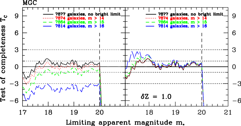
To this end, we take the MGC data-set (with no $(k+e)$-corrections applied) and introduce three, increasingly faint, artificial bright limits in apparent magnitude: $m_{b_{j}}>14$, $m_{b_{j}}>15$, and $m_{b_{j}}>16$ respectively. Fig. 4 (left) shows the resulting $T_{c}$ curves for the data-sets with these artificial bright limits, but where $T_{c}$ was computed assuming no bright limit. The plots clearly show that, as the bright limit is made progressively fainter, the computed value of $T_{c}$ deviates more strongly from the behaviour expected for a complete data-set. This trend is as expected: as can be seen in Fig. 1, the presence of the bright limit breaks the separability of the $M$ and $Z$ distributions for observable galaxies. Hence, if the bright limit is ignored then the computed value of $T_{c}$ will be systematically biased.
We now impose the same artificial bright limits as before but apply our generalised $T_{c}$ method which accounts for a bright and faint limit [see Fig. 4 (right)]. It is evident from this plot that, even with a bright magnitude limit as faint as $m_{b_{j}}=16$, the performance of the $T_{c}$ statistic at fainter magnitudes is largely unaffected, showing consistent behaviour for all the bright limits considered.

5.2 Testing the SDSS-DR1 dataset

Figure 5: Performance of the $T_{c}$ statistic applied, as an illustrative example, to the SDSS-DR1 early-type elliptical galaxies. In the left panel we compute $T_{c}$ using our extended method, fixing the bright magnitude limit to equal the published value of $14.55$ mag. We see that, in this case, the behaviour of $T_{c}$ is consistent with magnitude completeness up to and including the published faint limit of $17.45$ mag., but the statistic drops rapidly thereafter – indicating the sharp onset of magnitude incompletness. In the right hand panel, on the other hand, we compute $T_{c}$ following Rauzy (2001) – i.e. assuming a faint magnitude limit only. As anticipated, we see that the test statistic deviates very strongly from its expected value for a complete data-set at magnitudes which are much brighter than the published faint magnitude limit (although it is worth noting that $T_{c}$ still decreases even more rapidly once the published faint limit is exceeded).

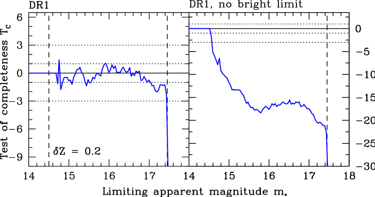
As previously discussed, the SDSS data-set has both a published bright and faint apparent magnitude limit of $m_{r}=14.55$ and $m_{r}=17.45$ mag. respectively. We, therefore, tested the completeness of the DR1 early type galaxies using our generalised $T_{c}$ statistic which accounts for both a faint and bright limit. As an illustration, we chose to fix the bright limit of the SDSS data-set to be equal to the published value, and computed the $T_{c}$ statistic as a function of the trial faint magnitude limit. We could, alternatively, have fixed the value of faint magnitude limit and computed the value of $T_{c}$ for different trial values of the bright limit, or indeed we could have treated simultaneously both the faint and bright limits as free parameters. However, the case we present is sufficient to illustrate our method. Fig. 5 (left) shows the resulting $T_{c}$ curve. We see that our results are in agreement with the published faint magnitude limit – i.e. the behaviour of $T_{c}$ is consistent with magnitude completeness up to and including a sharp, faint limit of $m_{r}=17.45$ mag., followed immediately by the strongly negative behaviour expected for an incomplete sample at fainter magnitudes.

The right-hand panel of Fig. 5 shows the $T_{c}$ curve computed using the traditional Rauzy method with a faint limit only. Here the results show a similar trend to that seen for the MGC data-set with an artificially imposed bright limit section, and further underlines to importance of correctly accounting for a bright and faint limit when both are present in the data. In a future paper we will explore in more detail the completeness of not only the current SDSS data releases, but also how that completeness varies with bandpass.

Figure 6: Performance of the $T_{c}$ statistic applied to our 2dFGRS sample. In the left hand panel we compute $T_{c}$ assuming only a faint magnitude limit, for both uncorrected magnitudes and after applying various different $(k+e)$-corrections. Note that several anomalous features are apparent, which are strongly discrepant from the behaviour of the test statistic expected for a complete sample. Moreover, $T_{c}$ begins to drop very sharply around $m\simeq 19.0$ mag. – significantly brighter than the published faint magnitude limit of $19.45$ mag. In the right hand panel we include the effect of a bright apparent magnitude limit, adopting for simplicity a value equal to the apparent magnitude of the brightest galaxy in our sample. The resulting $T_{c}$ curve (shown for uncorrected magnitudes and computed assuming a fixed ‘slice’ width of $\delta Z=0.8$ in distance modulus) is now entirely consistent with magnitude completeness up to and including the published faint limit, but drops very sharply at fainter magnitudes.

Figure 7: Comparison of the $T_{c}$ and $T_{v}$ statistics computed for MGC (left panel), SDSS-DR1 (middle panel) and 2dFGRS (right panel). For the latter two surveys the same bright limits were adopted as in Figs. 5 and 6 respectively, and appropriate values for $\delta Z$ (for $T_{c}$) and $\delta M$ (for $T_{v}$) were chosen. Note the almost identical agreement of the test statistics in each case. To illustrate the robustness of this result, the MGC results are with $(k+e)$-corrections applied, the SDSS-DR1 results are with $K$-corrections only applied, while the 2dFGRS results are for uncorrected galaxy data.

5.3 The 2dFGRS Survey

We move finally to the 2dFGRS survey which, as discussed in the Data section, has a published faint limit of $m^{f}_{lim}=19.45$ mag.

5.3.1 The Rauzy method with a faint limit only

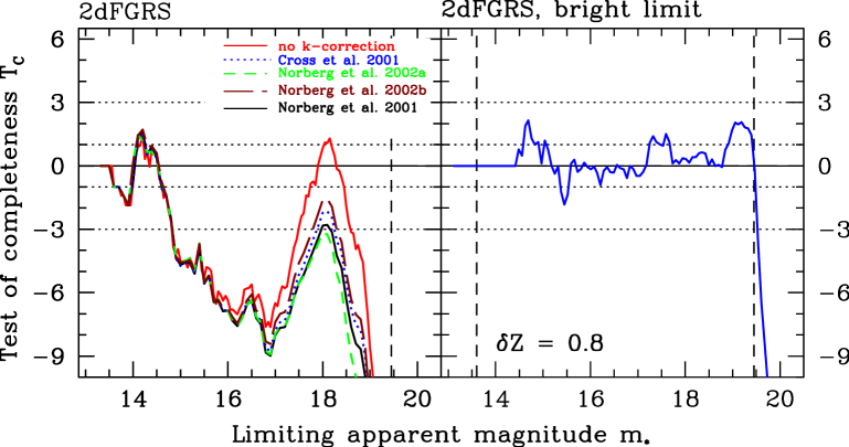
Our initial approach was to apply the traditional $T_{c}$ statistic to the 2dFGRS since the published literature on the survey gives no indication about the presence of a secondary bright limit. Fig. 6 (left) shows the behaviour of $T_{c}$ as a function of trial magnitude limit, $m^{\rm f}_{\star}$, for five different cases. The solid red curve represents the completeness test with with no $k$- or $e$-corrections applied. The remaining four curves show $T_{c}$ with various $(k+e)$- corrections applied to the 2dFGRS data-set, as shown in the figure key.

Consider firstly the uncorrected data-set (solid red curve). We see that for $m^{\rm f}_{\star}<14.85$ mag. the $T_{c}$ statistic appears to behave as we would expect for a complete sample (although of course this is at the cost of ‘throwing away’ most of the galaxies in the survey by imposing such a low value for the faint limit). However, for higher values of $m^{\rm f}_{\star}$ the statistic drops dramatically to a minimum value of nearly $8\sigma$ below its expectation value of zero at $m^{\rm f}_{\star}=16.90$ mag. As we continue to increase $m^{\rm f}_{\star}$, $T_{c}$ rises sharply to reach a peak at $m^{\rm f}_{\star}=18.15$ mag, beyond which the statistic drops dramatically again, exceeding $3\sigma$ below its expected value at $m^{\rm f}_{\star}=18.60$ – i.e. significantly brighter than the published magnitude limit of $m^{\rm f}_{\rm lim}=19.45$ mag.

Could the behaviour of $T_{c}$ be related to the fact that we have used an uncorrected data-set? To address this question consider now the remaining four curves; the dotted and short dashed curves correspond to the Cross (2001) and Norberg et al. (2001) global $(k+e)$-corrections respectively, whereas the long dashed and solid black curves correspond to the type-dependent $(k+e)$-corrections of Norberg (2002a, b). It is clear that the adoption of any of these corrections has very little effect on the completeness statistic compared with the uncorrected case. Indeed, if anything, the addition of $(k+e)$-corrections appears to yield a $T_{c}$ statistic which is more strongly inconsistent with a complete sample. This latter effect may be explicable in the same manner as for the corrected MGC magnitudes described in section 5.1, although it should be noted that the type-dependent $(k+e)$-corrections do not appear to perform significantly better than their global counterparts.

The fact that the value of $T_{c}$ differs from zero at many standard deviations over a wide range of trial faint magnitude limits is clear evidence that the distribution of $M$ and $Z$ for observable galaxies is not separable with these faint limits. The physical cause for this is not immediately clear; however, having demonstrated in the previous subsection the adverse impact on $T_{c}$ of not correctly accounting for a bright magnitude limit, we next apply our generalised test statistic to the 2dFGRS data-set.

5.3.2 2dFGRS with a bright limit

In the absence of a clear indication from the literature of what is an appropriate bright magnitude limit, we adopted the brightest galaxy in our subset (see §4.2.1), $m^{\rm b}_{\rm lim}=13.60$ mag. The right hand plot of Fig. 6 shows the $T_{c}$ curve obtained for the 2dFGRS (with no $k$- or $e$- corrections applied) as a function of trial faint limit, $m^{\rm f}_{\star}$, with $m^{\rm b}_{\rm lim}=13.60$ mag. We have used a $\delta Z$ = 0.8 (a small $\delta Z$ leads to low numbers of galaxies within the subsets, $S1$ and $S2$, making our test statistic prone to large statistical fluctuations and therefore less sensitive to a sharp cut in magnitude). The plot demonstrates a dramatic change in behaviour of the 2dF completeness, compared with the traditional $T_{c}$ statistic. By simply accounting for a bright limit – notwithstanding the fact that no published bright limit has been reported in the literature – we find that the 2dFGRS data-set is indeed complete to the published faint magnitude limit with no evidence for residual systematics.

6 APPLICATION OF THE $T_{v}$ STATISTIC

In the previous sections we introduced and applied our improved $T_{c}$ statistic, which accounts for both a faint and bright magnitude limit in assessing the completeness of a magnitude-redshift survey. In this section we apply the $T_{v}$ statistic, introduced in Section 3 above, to the same data-sets. Our $T_{v}$ statistic can be thought of as an improved, differential, version of the classical $\cal{V}$/$\cal{V}$_max test of galaxy evolution, which is generally presented in the literature as yielding a single number – the mean value of $\cal{V}$/$\cal{V}$_max averaged over all galaxies in the survey, adopting a given faint apparent magnitude limit and assuming that the underlying spatial distribution of galaxies is homogeneous. In contrast, we can compute $T_{v}$ as a function of an incrementally increasing $m^{\rm f}_{\star}$ (and/or indeed, if we wished, an incrementally decreasing bright limit, $m^{\rm b}_{\rm lim}$) and thus analyse our data-set via a series of progressively truncated subsets. Crucially, moreover, like the $T_{c}$ test and unlike the $\cal{V}$/$\cal{V}$_max statistic, $T_{v}$ has the important property of being independent of the spatial distribution of galaxies within the survey.

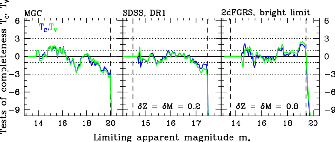
Fig. 7 shows a comparison of the $T_{v}$ and $T_{c}$ curves for all three surveys. The left hand plot is the MGC survey with $(k+e)$-corrections applied. The $T_{v}$ curve shows an almost identical match to the $T_{c}$ statistic. Similar behaviour is evident with SDSS-DR1 and 2dFGRS (middle and right plots). That $T_{v}$ and $T_{c}$ give a consistent indication of the completeness of these surveys should not be too surprising, since we are confident (at least once a bright limit is included in our analysis of 2dFGRS) that all three are well calibrated and well understood. Moreover, they are all relatively shallow in redshift range, which means that extinction and evolution corrections are not likely to impact too strongly on our assessment of their completeness (a fact which is supported by our results for $T_{c}$). However, one can ask under what conditions might the two statistics $T_{c}$ and $T_{v}$ diverge from each other?

Consider a galaxy, $i$, characterised by its ‘coordinates’ $(M_{i},Z_{i})$. We have two complementary ways of generating volume limited data-sets for such a pair:

• at fixed luminosity we can ask what redshift distribution will produce apparent magnitudes permitted by our selection criteria?

• alternatively, at fixed redshift we can ask what distribution of luminosities (i.e. what part of the underlying galaxy luminosity function) are we sampling, given our selection limits in apparent magnitude?

The former criterion resembles the procedure used to contruct the $T_{v}$ statistic, while the latter criterion is more closely related to the procedure used to construct $T_{c}$. This also implies that one might expect the two statistics to behave differently when evolution becomes important – simply because evolution will, of course, break the separability of the underlying joint distribution of $M$ and $Z$, i.e. the conditional distributions of $M$ at given $Z$ and $Z$ at given $M$ will no longer be simply equal to their marginal distributions. It seems likely, therefore, that an exploration of the systematic differences between $T_{c}$ and $T_{v}$ for deeper surveys may be an effective probe of evolution.

7 SUMMARY

We have developed the completeness test statistic, $T_{c}$, first introduced in Rauzy (2001), technique to account for the presence of both a faint and bright apparent magnitude limit in magnitude-redshift samples. We have applied it to the MGC, SDSS-DR1 and 2dFGRS surveys. Our results confirm the completeness of data-sets such as SDSS-DR1 (early types only) where a faint and bright limit is well defined and published in the literature. Specifically, we have demonstrated that SDSS-DR1 is complete in apparent magnitude up to the published magnitude limit of $m_{r}=17.45$ mag indicating no residual systematics. Similarly, the magnitude completeness of the MGC survey has also been confirmed up to its published limit of $m_{b_{j}}=20.0$ mag. Interestingly, however, we found that when we incorporated $(k+e)$-corrections to the MGC data-set, a noticeable (although not statistically significant) departure from the expected value of the $T_{c}$ statistic – and indeed from the computed value of $T_{c}$ for the uncorrected data – was observed close to the magnitude limit. A possible cause for this effect could be the mixing of galaxy populations to which a global $(k+e)$ is then applied – resulting in a slightly $blurred$ magnitude limit.

Our initial approach to the 2dF galaxy survey was to apply the original Rauzy test which accounts for a single, faint magnitude limit only. This was motivated by the current literature, in which $only$ a faint limiting magnitude of $m=19.45$ was well defined in the survey. However, our the application of our $T_{c}$ test reveal that the 2dFGRS is strongly inconsistent with being complete in apparent magnitude unless a secondary bright limit ($m=13.6$ in our subset) is included.

Finally, we have also developed another variant on the original Rauzy $T_{c}$ completeness statistic, which we denote by $T_{v}$, based on the cumulative distance distribution of galaxies in a magnitude-redshift survey. We find that $T_{v}$ has potential advantages over the widely used $\cal{V}$/$\cal{V}$_max test: not least, the $T_{v}$ statistic retains the same properties as that of $T_{c}$ – i.e. is independent of the spatial distribution of galaxies within the survey. Furthermore, we have shown by example, that $T_{v}$ – when applied to the same well calibrated and relatively shallow survey samples as $T_{c}$ – produces almost identical results to that of the $T_{c}$ statistic. Our future work in this area will explore the application of $T_{v}$ and $T_{c}$ to deeper surveys, where evolution and $k$-corrections become more important issues, to investigate the potential of these two statistics as diagnostics of luminosity and density evolution.

References

- Abazajian (2003) Abazajian, K., et al..: 2003, AJ 126, 2081
- Bernardi et al. (2003) Bernardi, M., Sheth, R. K., Annis, J., Burles, S., Eisenstein, D. J., Finkbeiner, D. P., Hogg, D. W., Lupton, R. H., Schlegel, D. J., SubbaRao, M., Bahcall, N. A., Blakeslee, J. P., Brinkmann, J., Castander, F. J., Connolly, A. J., Csabai, I., Doi, M., Fukugita, M., Frieman, J., Heckman, T., Hennessy, G. S., Ivezić, Ž., Knapp, G. R., Lamb, D. Q., McKay, T., Munn, J. A., Nichol, R., Okamura, S., Schneider, D. P., Thakar, A. R., and York, D. G.: 2003, AJ 125, 1817
- Bernardi et al. (2005) Bernardi, M., Sheth, R. K., Nichol, R. C., Schneider, D. P., and Brinkmann, J.: 2005, AJ 129, 61
- Binggeli et al. (1988) Binggeli, B., Sandage, A., and Tammann, G. A.: 1988, Annu.Rev.Astron.Astrophysics 26, 509
- Blanton et al. (2003) Blanton, M. R., Lin, H., Lupton, R. H., Maley, F. M., Young, N., Zehavi, I., and Loveday, J.: 2003, AJ 125, 2276
- Cross (2001) Cross, N., et al..: 2001, MNRAS 324, 825
- Cross et al. (2004) Cross, N. J. G., Driver, S. P., Liske, J., Lemon, D. J., Peacock, J. A., Cole, S., Norberg, P., and Sutherland, W. J.: 2004, MNRAS 349, 576
- Driver et al. (2005) Driver, S. P., Liske, J., Cross, N. J. G., De Propris, R., and Allen, P. D.: 2005, MNRAS 360, 81
- Efron and Petrosian (1992) Efron, B. and Petrosian, V.: 1992, ApJ 399, 345
- Efron and Petrosian (1998) Efron, B. and Petrosian, V.: 1998, ArXiv Astrophysics e-prints
- Efstathiou et al. (1988) Efstathiou, G., Ellis, R. S., and Peterson, B. A.: 1988, MNRAS 232, 431
- Eisenstein (2001) Eisenstein, D. J., et al..: 2001, AJ 122, 2267
- Fukugita et al. (1996) Fukugita, M., Ichikawa, T., Gunn, J. E., Doi, M., Shimasaku, K., and Schneider, D. P.: 1996, AJ 111, 1748
- Gunn (1998) Gunn, J. E., et al..: 1998, AJ 116, 3040
- Hogg et al. (2001) Hogg, D. W., Finkbeiner, D. P., Schlegel, D. J., and Gunn, J. E.: 2001, AJ 122, 2129
- Hubble (1926) Hubble, E. P.: 1926, ApJ 64, 321
- Hudson and Lynden-Bell (1991) Hudson, M. J. and Lynden-Bell, D.: 1991, MNRAS 252, 219
- Lupton (2001) Lupton, R., et al..: 2001, in F. R. Harnden, Jr., F. A. Primini, and H. E. Payne (eds.), ASP Conf. Ser. 238: Astronomical Data Analysis Software and Systems X, pp 269–+
- Lynden-Bell (1971) Lynden-Bell, D.: 1971, MNRAS 155, 95
- Maddox et al. (1990) Maddox, S. J., Efstathiou, G., Sutherland, W. J., and Loveday, J.: 1990, MNRAS 243, 692
- Norberg (2002a) Norberg, P., et al..: 2002a, MNRAS 336, 907
- Norberg (2002b) Norberg, P., et al..: 2002b, MNRAS 332, 827
- Norberg et al. (2001) Norberg, P., Baugh, C. M., Hawkins, E., Maddox, S., Peacock, J. A., Cole, S., Frenk, C. S., Bland-Hawthorn, J., Bridges, T., Cannon, R., Colless, M., Collins, C., Couch, W., Dalton, G., De Propris, R., Driver, S. P., Efstathiou, G., Ellis, R. S., Glazebrook, K., Jackson, C., Lahav, O., Lewis, I., Lumsden, S., Madgwick, D., Peterson, B. A., Sutherland, W., and Taylor, K.: 2001, MNRAS 328, 64
- Pier et al. (2003) Pier, J. R., Munn, J. A., Hindsley, R. B., Hennessy, G. S., Kent, S. M., Lupton, R. H., and Ivezić, Ž.: 2003, AJ 125, 1559
- Rauzy (2001) Rauzy, S.: 2001, MNRAS 324, 51
- Rauzy et al. (2001) Rauzy, S., Hendry, M. A., and D’Mellow, K.: 2001, MNRAS 328, 1016
- Sandage et al. (1979) Sandage, A., Tammann, G. A., and Yahil, A.: 1979, ApJ 232, 352
- Schmidt (1968) Schmidt, M.: 1968, ApJ 151, 393
- Smith (2002) Smith, J. A., et al..: 2002, AJ 123, 2121
- Stoughton (2002) Stoughton, C., et al..: 2002, AJ 123, 485
- Strauss (2002) Strauss, M. A., et al..: 2002, AJ 124, 1810
- York (2000) York, D. G., et al..: 2000, AJ 120, 1579