X-ray Variability Coherence in the Time Domain

Abstract

A technique for calculation of variability coherence at different timescales performed directly in the time domain is introduced. Simulations are made to compare the coherence spectrum derived by the time domain technique with the coherence function by Fourier analysis. The results indicate that in comparison with the Fourier analysis the time domain technique is more powerful for revealing signal coherence in noisy data. We apply the time domain technique to the real data of the black hole binaries Cygnus X-1 and GX 339-4 and compare the results with their Fourier coherence spectra.

1 Introduction

The complex aperiodic variability of high-energy emission shown in different time scales is a common character for X-ray binaries and super massive black holes. Temporal analysis is an important approach to study undergoing physics in objects from observed light curves. The spectral lag between variation signals in different energy bands provides useful information on their producing and propagating processes in celestial objects. Besides the time lag, the spectral coherence, a measure of the degree of linear correlation between two light curves in different energy bands, is another useful quantity to provide constraints on models of physical processes in observed objects. For studying variability coherence in the frequency domain, the coherency function – the normalized average amplitude of the cross power density as a function of Fourier frequency – can be used. Vaughan and Nowak (1997) have presented a procedure for estimating the coherence function in the presence of counting noise, which has been applied to studying black hole candidates (e.g. Nowak & Vaughan 1996; Vaughan & Nowak 1997; Cui, Zhang & Chen 2000; Nowak et al. 2001; Nowak, Wilms & Dove 2002; Ji et al. 2003).

The time domain quantity corresponding to the coherence in the frequency domain is the coefficient of linear correlation between two light curves in different energy bands. The correlation coefficient has not been extensively applied in temporal analysis as the coherence function in the frequency domain. One of the reasons is that the variability is caused by various physical processes at different timescales, a single value of correlation coefficient from two observed light curves is not enough to provide measures of association between complex variables. What needed is a distribution of correlation coefficient over timescales. Here we present a procedure for deriving the coherence spectrum in the time domain, or a timescale spectrum of the correlation coefficient for a complex process in the presence of background noise and compare the coherence spectrum in the time domain with the Fourier frequency-dependent function of coherence by simulation in §2. In our simulation, the result from the time domain technique is consistent with the coherence function obtained from the Fourier analysis when the signal to noise ratio is high. In general, the time domain technique can provide a more accurate and stable result than the Fourier analysis. We apply the time domain technique to the black hole X-ray binaries Cygnus X-1 and GX 339-1 and present the results in §3 and give discussion on timelag effect in §4.

2 Timescale Spectrum of Correlation Coefficient

A proper statistic for measuring the degree of linear correlation between variations in two $N$-point signal counting series $x_{s}(i)$ and $y_{s}(i)$ is their correlation coefficient

$$r=\frac{\sum_{i=1}^{N}(x_{s}(i)-\overline{x}_{s})(y_{s}(i)-\overline{y}_{s})/N}{\sigma(x_{s})\sigma(y_{s})}.$$ (1)

For two observed lightcurves $x(i)=x_{s}(i)+x_{n}(i)$ and $y(i)=y_{s}(i)+y_{n}(i)$ with independent noise $x_{n}$ and $y_{n}$ respectively, we have

$$\sum_{i}(x(i)-\overline{x})(y(i)-\overline{y})=\sum_{i}(x_{s}(i)-\overline{x}_{s})(y_{s}(i)-\overline{y}_{s}),$$

and

$$\sigma^{2}(x)=\sigma^{2}(x_{s})+\sigma^{2}(x_{n}),\hskip 11.38109pt\sigma^{2}(y)=\sigma^{2}(y_{s})+\sigma^{2}(y_{n}),$$

then the signal’s correlation coefficient can be calculated as

$$r=\frac{\sum_{i=1}^{N}(x_{s}(i)-\overline{x}_{s})(y_{s}(i)-\overline{y}_{s})/N}{\sigma(x_{s})\sigma(y_{s})}=\frac{\sum_{i=1}^{N}i(x(i)-\overline{x})(y(i)-\overline{y})/N}{\sqrt{\sigma^{2}(x)-\sigma^{2}(x_{n})}{\sqrt{\sigma^{2}(y)-\sigma^{2}(y_{n})}}}~{}.$$ (2)

It should be pointed out that one can not take two so called “background-subtracted lightcurves” as signal’s lightcurves $x_{s}$ and $y_{s}$ to calculate the correlation coefficient simply by Eq. (1), because background lightcurves given by a database are usually smoothed curves not including the fluctuation of real noise at shorter timescales.

We apply a timescale analysis technique (Li, Feng & Chen 1999; Li 2001; Li et al. 2004) to calculate correlation coefficients for different timescales from two observed lightcurves. From an original lightcurve $x(j;\delta t)~{}(j=1,2,\cdots)$ with a time resolution $\delta t$, we can construct $M$ different lightcurves with the same larger time step $\Delta t=M\delta t$ by combining $M$ successive bins

$$x_{m}(i;\Delta t)=\sum_{j=(i-1)M+m}^{iM+m-1}x(j;\delta t)~{},\hskip 14.22636pt(m=1,\cdots,M)~{},$$ (3)

where the combination starts from the $m$th bin of the original lightcurve. From two simultaneously observed counting series $x(j;\delta t)$ and $y(j;\delta t)$, the correlation coefficient $r(\Delta t)$ for a certain timescale $\Delta t=M_{\Delta t}\delta t$ can be calculated by

$$r(\Delta t)=\frac{1}{M_{\Delta t}}\sum_{m=1}^{M_{\Delta t}}\frac{\sum_{i=1}^{N}(x_{m}(i)-\overline{x}_{m})(y_{m}(i)-\overline{y}_{m})/N}{\sqrt{\sigma^{2}(x_{m})-\sigma^{2}(x_{n})}{\sqrt{\sigma^{2}(y_{m})-\sigma^{2}(y_{n})}}}~{}.$$ (4)

The total observation period is divided into $L$ segments. The correlation coefficient $r_{k}(\Delta t)$ is calculated by Eq. (4) for a pair of lightcurves on each time segment $k$ separately. The average $\overline{r}(\Delta t)=\sum_{k=1}^{L}r_{k}(\Delta t)/L$ and its standard deviation $\sigma(\overline{r})$ are defined as the coherence coefficient for the timescale $\Delta t$ and its error.

To check the procedure described above and compare it with the Fourier coherence function we produce two 1000 s signal time series, $x_{s}$ and $y_{s}$, with time bin $\delta t=1$ ms sampled from a two-dimensional normal distribution

$$p(x_{s},y_{s}) = \frac{1}{2\pi\sigma(x_{s})\sigma(y_{s})\sqrt{1-\rho^{2}}}\exp\left\{-\frac{1}{2(1-\rho^{2})}\left[\left(\frac{x_{s}-\langle x_{s}\rangle}{\sigma(x_{s})}\right)^{2}\right.\right.$$ (5)

$$\left.\left.-2\rho\frac{x_{s}-\langle x_{s}\rangle}{\sigma(x_{s})}\frac{y_{s}-\langle y_{s}\rangle}{\sigma(y_{s})}+\left(\frac{y_{s}-\langle y_{s}\rangle}{\sigma(y_{s})}\right)^{2}\right]\right\}~{},$$

where $\langle x_{s}\rangle,\sigma(x_{s}),\langle y_{s}\rangle,\sigma(y_{s})$ are means and standard deviations of $x_{s}$ and $y_{s}$ respectively, and $\rho$ is the correlation coefficient between $x_{s}$ and $y_{s}$. By giving these parameters in Eq. (5), we are able to produce two signal time series with a certain correlation coefficient. To simplify, we specify $\langle x_{s}\rangle=\langle y_{s}\rangle=49$, $\sigma(x_{s})=\sigma(y_{s})=7$. The correlation coefficient $\rho$ in Eq. (5) is the theoretical value of coherence, and it is used to compare with results of time domain coherence and Fourier coherence function. We add independent Poisson noise $x_{n}$ and $y_{n}$ on the signal series $x_{s}$ and $y_{s}$ respectively to get simulated lightcurves $x=x_{s}+x_{n}$ and $y=y_{s}+y_{n}$. Different signal to noise ratio (SNR) could be set by adjusting the mean of independent Poisson noise. The simulated lightcurve is divided into ten segments, each has a length of 100 s. For each segment, coherences at different timescales are calculated by Eq. (4) and Fourier coherence coefficients at different frequencies are also computed with the procedure described by Vaughan and Nowak (1997). Finally, the average and its standard deviation are computed from the ten time domain coherences and Fourier coherence coefficients separately.

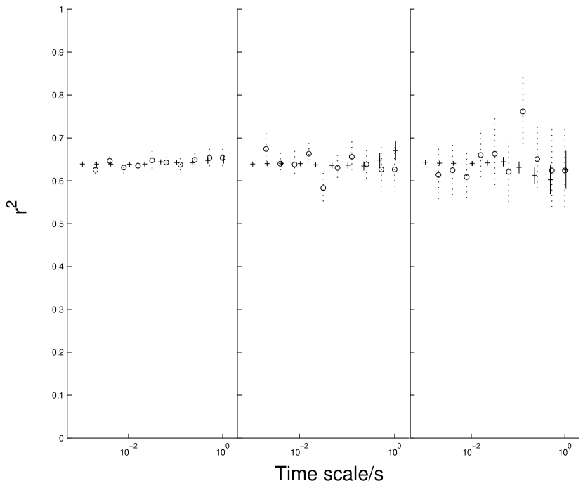
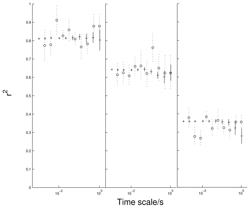
Figure 1 shows coherence spectra from simulated light curves with $\rho=0.8$ and SNR = 5, 2 and 1 separately, where Fourier coherence function in the frequency domain are transformed into the time domain by $timescale=1/frequency$. From Fig. 1 we can see that, in comparing with Fourier coherence functions, time domain coherence distributions are more consistent and accurate. For the case of low SNR, Fourier coherence functions fluctuate seriously and have a large error bar, while the time domain procedure has a better capability to reveal a given coherence, especially at short timescales. Figure 2 show the results for a certain SNR = 1 and different $\rho=0.9$, 0.8 and 0.6 respectively, indicating that the time domain procedure is more powerful to reveal lower measured coherence.

Figure 1: Coherence between two simulated lightcurves with a given signal coherence $r^{2}=0.64$ and different SNR. From left to right, SNR = 5, 2 and 1 respectively. Plus sign and solid line represent the coherence and its deviation obtained by the time domain technique. Circle and dotted line show Fourier coherence function.

Figure 2: Coherence between two simulated lightcurves with a given SNR = 1 and different signal correlation coefficients. From left to right, the signal correlation coefficient $r^{2}=0.81$, 0.64, and 0.36 respectively. Plus sign and solid line represent the coherence and its deviation obtained by the time domain technique. Circle and dotted line show Fourier coherence function.

The test and comparison are extended to different signal distributions other than the binormal one. The joint probability density function of binormal distribution can be factorized into two factors

$$p(x,y)=p(x)p(y|x)~{},$$ (6)

where

$$p(x)=\frac{1}{\sqrt{2\pi}\sigma_{x}}\exp\left[-\frac{1}{2}\left(\frac{x-\langle x\rangle}{\sigma_{x}}\right)^{2}\right]~{},$$ (7)

and

$$p(y|x)=\frac{1}{\sqrt{2\pi}\sigma_{y}\sqrt{1-\rho^{2}}}\exp\left[-\frac{1}{2}\left(\frac{y-\langle y\rangle-\rho\frac{x-\langle x\rangle}{\sigma_{x}}\sigma_{y}}{\sigma_{y}\sqrt{1-\rho^{2}}}\right)^{2}\right]~{}.$$ (8)

The first factor $p(x)$ of Eq. (6) is a one-dimensional Gaussian density function of the variable $x$ which is independent of $y$. The second factor $p(y|x)$ is also a Gaussian density but with average $\overline{y}+\rho\frac{x-\overline{x}}{\sigma_{x}}\sigma_{y}$, standard error $\sigma_{y}\sqrt{1-\rho^{2}}$ and the correlation coefficient $\rho$ between x and y, which can be seen as a conditional density of $y$ given $x$. With Eq. (6) we can produce a pair of time series with a given correlation coefficient $\rho$ with a density function $p(x)$ different to Gaussian by sampling $x$ from the density $p(x)$ and $y$ from the density of Eq. (8). The exponential distribution, uniform distribution and Poisson distribution are adopted as $p(x)$ to produce correlated pairs of time series separately, and then compute their coherence distributions in the time domain and their Fourier correlation functions. All results are similar with Fig. 1 and Fig. 2, showing that the time domain procedure is an effective approach to coherence analysis.

3 X-ray Coherence of Black Hole Binaries

Here we apply the time domain technique of coherence analysis to two black hole candidates, Cyg X-1 in the low state and GX 339-4 in the low and high states. We use observational data from PCA/$RXTE$. PCA/$RXTE$ observation has dead time $10\mu s$ much smaller than time resolution 1ms of original lightcurves we use in this paper. And for Cyg X-1, dead-time affection is about $1\%$ (Maccarone and Coppi 2000), so it could be ignored.

Variabilities in lightcurves observed for an astronomical object are usually caused by various processes at different timescales with different coherences. The coherence coefficient $r(\Delta t)$ calculated by Eq. (4) reflects not only the variation property on the timescale $\Delta t$, but is also affected by that on larger ones up to the total time period used in the calculation. To limit the effect of larger timescales we divide the total observation period into segments, each has a duration just 10$\Delta t$. The resultant correlation coefficient should be then related to the limited time scale region of $\Delta t-10\Delta t$.

In our calculation for Cyg X-1 and GX 339-4 data, for a given time bin $\Delta t$ the studied observation period is divided into segments with a duration of 10$\Delta t$ each and the coherence coefficient is calculated for each segment by using Eq. (4). The all segments are divided into ten groups with the segment numbers in each group being nearly equal to each other. We calculate 10 avarage coherence coefficients $r_{k}(\Delta t)$ for each group $k~{}(k=1,\dots,10)$ respectively and take their average $r(\Delta t)=\sum_{k=1}^{10}r_{k}(\Delta t)/10$ and the standard deviation $\sigma[r(\Delta t)]$ as the final result of the observation. The Fourier coherence coefficients and their average and the standard deviation of the average are also calculated from the 10 time groups. The results are shown in Figure 3. For both Cyg X-1 and GX 339-4 in the low state shown in the left and middle panels of Fig. 3, both Fourier coherence and time domain coherence show similar trend of change from near-perfect coherence at large time scale to low coherence at small time scale. Two other black hole candidates, XTE J1550-564 (Cui, Zhang and Chen 2000) and GRS 1915+105 (Ji et al. 2003), have Fourier coherence function with near-unity coherence at large time scale and low coherence at small time scale. We also apply the time domain technique to these sources and get similar results. As the coherence is much more easily to be lost than maintained, only when one linear physical process is involved could coherence be preserved (Vaughan & Nowak 1997). Any nonlinear process or more than one independent linear processes involved could degrade coherence. The near-perfect coherence at large time scale may provide a strong evidence that there is a powerful physical process in these sources with a large characteristic timescale dominates the emission of photons in the studied energy bands.

It is a remarkable feature that all the values of time domain coherence are very low in the whole studied timescale range for GX 339-4 in the high state, shown in the right panel of Fig. 3, indicating that there is only little relationship between variabilities of 2-5 keV and 5-7 keV emissions of GX339-4 in its high state.

Figure 3: Variability coherence for black hole X-ray binaries. Plus: coherence obtained by the time domain technique. Circle: Fourier coherence function. Left panel: Cyg X-1 in the low state, PCA/$RXTE$ observation in Dec-17-1996, 2-5 keV vs. 5-13 keV. Middle panel: GX 339-4 in the low state, PCA/$RXTE$ observation in Sep-19-1997, 2-6 keV vs. 6-8 keV. Right panel: GX 339-4 in the high state, PCA/$RXTE$ observation in Jan-17-1998, 2-5 keV vs. 5-7 keV.

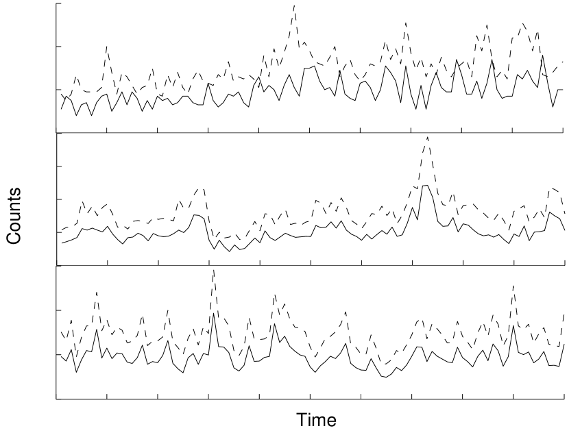
To see whether the relationship between variabilities of two light curves coincides with the time domain coherence computed from them, we simultaneously plot two observed light curves of Cyg X-1 in two energy bands for different time scales at the same time period, shown in Figure 4. From Fig. 4 one can see that the time domain coherence calculated by Eq. (4) can reflect the real strength of the linear relationship between two light curves.

Figure 4: Lightcurve segments of Cyg X-1 in the low state, PCA/$RXTE$ observation in Dec-17-1996. $Solid~{}line$: 2-5 keV, $Dashed~{}line$: 5-13 keV. Top panel: 10 ms time bin, time domain coherence in Fig. 3 is $\sim 0.4$. Middle panel: 100 ms time bin, coherence $\sim 0.9$. Bottom panel: 1000 ms time bin, coherence is very near to unit.

4 Discussion

The Fourier coherence function $r(f)$ of two lightcurves $x$ and $y$ is defined in the space of Fourier frequency

$$r(f)=\frac{|\left<C(f)\right>|}{\sqrt{\left<|X(f)|^{2}\right>\left<|Y(f)|^{2}\right>}}~{}.$$ (9)

Where, $X(f)$ and $Y(f)$ are the Fourier transforms of $x$ and $y$ respectively, the cross spectrum $C(f)=X^{*}(f)Y(f)$, and angle brackets denote an average over the used segments of light curve. If the ratio of two Fourier transforms at a frequency $f$, $H(f)=X(f)/Y(f)$, is the same for all segments of the two processes, or, equivalently

$$y(t)=\int h(t-\tau)x(\tau)d\tau~{},$$ (10)

then $r(f)=1$, the processes are said to be coherent at frequency $f$. But the unit coherence in the time domain, $r(\Delta t)=1$, indicates a linear correlation between the variabilities of intensity in the two energy bands on the timescale $\Delta t$

$$y(i;\Delta t)=hx(i;\Delta t)~{},\hskip 14.22636pt(i=1,\dots,N_{T})~{},$$ (11)

where $h$ is a constant during the observation period $T=N_{T}\Delta t$, which is a stronger constraint than Eq. (10) from an unit coherence, $r(f)=1$, in the frequency domain. It is an advantage for Fourier coherence function that it can obtain coherence at all frequencies simultaneously and exactly, because amplitude at all frequencies could be obtained independently from Fourier transformation of original lightcurve. Improved Fourier coherence function (Vaughan & Nowak 1997) can calculate coherence of noisy lightcurves and uncertainty as well. While the coherence coefficient calculated in the time domain by Eq. (4) can be confined in only a timescale region, $\Delta t-N\Delta t$ with $N$ being the number of time bins in a calculated time segment, and the error of the average coherence coefficient is estimated by the statistical deviation in coherence coefficients of different time segments.

Spectral time lags are usually existed in observed processes. To calculate the time domain coherence $r(\Delta t)$, one should firstly derive their timescale spectrum of time lag, then make time lag correction for light curves at the timescale $\Delta t$. But, in practice, the coherence derived by the time domain technique is not sensitive to the spectral time lag in analyzing real observational data. From lightcurves of Cyg X-1 in its low state in energy band 2-5 keV and 5-13 keV observed by PCA/$RXTE$, we use the modified cross-correlate function (MCCF) (Li, Feng & Chen 1999; Li et al. 2004) to calculate the spectral time lag, the result is similar to what obtained from Fourier analysis (Nowak et al 1999). Then we calculate time domain coherences between the two lightcurves with and without time lag correlation separately. The result shown in Fig. 5 does not indicate any essential effects of the spectral lag on the time domain coherence. To see how seriously time lag could affect results of time domain coherence, we make a modification to the original observed lightcurves to produce an artificial deviation: the band 5-13 keV lags behind the band 2-5 keV by 10 times of time lag measured from the observed lightcurves by MCCF, then calculate time domain coherences between the modified lightcurves. As we can see in Fig. 5, only a litter deviation can be found between the result from the original lightcurves and the modified ones. We also test other data used in this paper to see whether Fig. 5 is only an exception, the results turns out to be that although the spectral time lag exists in most data, it has just little influence to the coherence obtained by the time domain technique.

Figure 5: X-ray coherence obtained by the time domain technique. Cyg X-1 in the low state, PCA/$RXTE$ observation in Dec-17-1996, 2-5 keV vs. 5-13 keV. Circle: from original observed lightcurves. Cross: from lightcurves after spectral timelag correction. Plus: from modified lightcurves whose timelag is artificially amplified by 10 times.

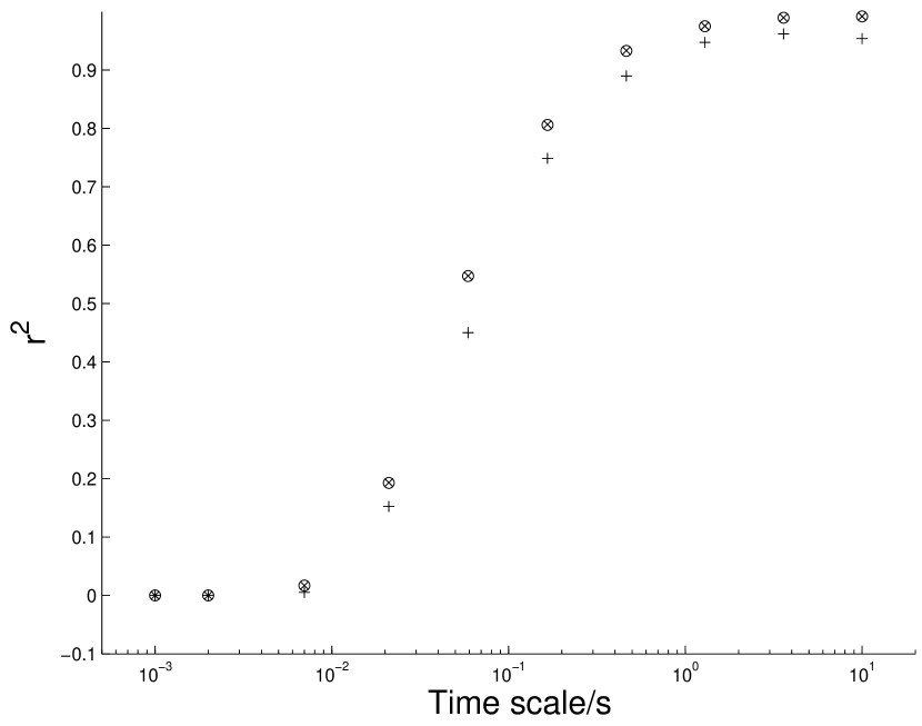
To understand reasons of insensitivity of time domain coherence to spectral timelag in observed X-ray data, we make simulation studies. Two 1000 s lightcurves with 1 ms time bin and a given correlation coefficient $\rho=0.8$ (or expected coherence $r^{2}=0.64$) are produced by sampling from the two-dimensional normal distribution Eq. (5) described in §2. One of the lightcurves is then artificially shifted by 10 ms. We use MCCF to derive timescale distribution of time lags and calculate time domain coherences between the two lightcurves with and without timelag correction. The results are shown in the left panel of Figure 6. We can see that, though the effect of spectral timelag can not be neglected in general, the difference of coherences obtained with and without timelag correction is small at large timescale. For deriving time domain coherences at large timescales, we need to reconstruct original lightcurves with a larger time bin (see the details in §2), which impairs the effect of a timelag which is much smaller than the time bin. Spectral timelags measured at a timescale are usually much shorter than the timescale itself. For example, the X-ray time lag of Cyg X-1 between 2-5 keV and 5-13 keV at the timescale of 1 s (or frequency of 1 Hz) is only about 10 ms. From the left panel of Fig. 6 we can see that the effect of timelag on time domain coherence is small when timelag is much smaller than time bin.

Figure 6: Spectral timelag effect on coherence obtained by the time domain technique. Circle : no timelag correction. Plus: after timelag correction. Left panel: coherence between two simulated lightcurves based on two-dimensional normal distribution model with timelag 10ms at all time scale, the given coherence is $r^{2}=0.64$. Right panel: coherence between two simulated lightcurves based on shot model with timelag 10ms at all time scale.

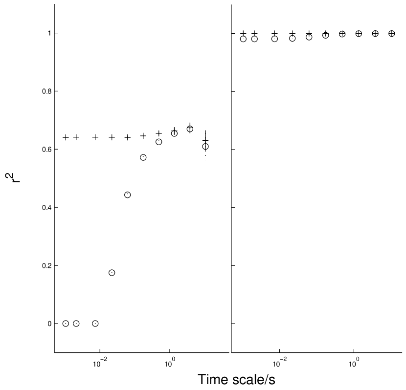
The correlation existed in successive time bins in observed lightcurves may be another reason of the insensitivity of time domain coherence to spectral timelag in observed X-ray data. The right panel of Fig. 6 shows results from two simulated lightcurves based on shot model with 10 ms timelag. We produce a 1000 s lightcurve with 1 ms time bin consisted of random shots similar to what observed from Cyg X-1 (Feng, Li & Chen 1999). The front of the shot is represented by a single exponential and the time constant of both ascending and descending front is 70 ms. The interval between two successive shots follows an exponential distribution with an average of 450 ms. The above produced lightcurve is shifted by 10 ms to create the second one. The right panel of Fig. 6 shows coherence spectra derived by the two lightcurves with and without timelag correction. From Fig. 6 we see that the timelag effect on time domain coherence for lightcurves produced by shots (right panel) is much smaller than that for lightcurves sampled from two-dimensional normal distribution (left panel). This is because successive bins in a lightcurve consisted of shots have a strong connection.

In summary, we propose a time domain technique in this paper to calculate variability coherence for different timescales. In general, the time domain coherence distribution is consistent with the Fourier coherence function, but more reliable for the case of low signal to noise ratio and more powerful to reveal lower coherence. In practical data analysis, the effect of spectral time lags on the time domain coherence can be neglected. This technique provides an useful tool for temporal analysis.

References

- Bendat, J., & Piersol, A. (1986) Bendat, J., & Piersol, A. 1986, Random Data: Analysis and Measurement Procedures
- Cui, Zhang & Chen (2000) Cui W., Zhang S.N. & Chen W. 2000, ApJ, 531, L45
- Feng, Li & Chen (1999) Feng Y.X., Li, T.P. & Chen L. 1999, ApJ, 514, 373
- Ji et al. (2003) Ji J.F., Zhang S.N., Qu J.L. & Li T.P. 2003, ApJ, 584, L23
- Li T.P. (2001) Li T.P. 2001, Chinese J. Astron. Astrophys., 1, 313; astro-ph/0109468
- Li, Feng & Chen (1999) Li, T.P., Feng Y.X. & Chen L. 1999, ApJ, 521, 789
- Li T.P. et al. (2004) Li T.P., Qu J.L., Feng H., Song L.M., Ding G.Q. & Chen L. 2004, Chinese J. Astron. Astrophys., 4, 583; astro-ph/0407458
- (8) Maccarone,T.J & Coppi,P.S. 2000, ApJ, 537, L107
- Nowark & Vaughan (1996) Nowark,M.A. & Vaughan,B.A. 1996, MNRAS, 280, 227
- Nowark et al. (1999) Nowark, M.A., Vaughan, B.A., Wilms, J., Dove, J.B. & Begelman, M.C. 1999, ApJ, 510, 874
- Nowark et al. (2001) Nowark,M.A., Wilms, J., Heindl W.A., Pottschmidt K., Dove,J.B. & Begelman,M.C. 2001, MNRAS, 320, 316
- Nowark,M.A., Wilms,J. and Dove,J.B. (2002) Nowark,M.A., Wilms,J. & Dove,J.B. 2002, MNRAS, 332, 856
- Vaughan,B.A. and Nowark,M.A. (1997) Vaughan,B.A. & Nowark,M.A. 1997, ApJ, 474, L43