Predicting solar cycle 24 with a solar dynamo model
Abstract
Whether the upcoming cycle 24 of solar activity will be strong or not is being hotly debated. The solar cycle is produced by a complex dynamo mechanism. We model the last few solar cycles by ‘feeding’ observational data of the Sun’s polar magnetic field into our solar dynamo model. Our results fit the observed sunspot numbers of cycles 21-23 extremely well and predict that cycle 24 will be about 35% weaker than cycle 23.
Solar activity affects our space environment, thereby influencing various aspects of human life [1]. So it is vitally important to develop capabilities for predicting strengths of the 11-year cycles of solar activity. It has been believed for some time that the Sun’s polar magnetic field at the preceding minimum gives an indication of the strength of the next solar cycle [2]. The weakness of the present polar field has already led to predictions that cycle 24 will be the weakest cycle in 100 years [ 3, 4]. Since the solar cycle is produced by a dynamo mechanism, one would like to make a prediction of cycle 24 from a detailed solar dynamo model also. The only previous dynamo-based prediction is that cycle 24 will be one of the strongest cycles [5]. Our aim is to generate an independent prediction for cycle 24 from a different dynamo model by a different methodology. We identify the Babcock–Leighton process for poloidal field generation as the main source of randomness in solar cycles. A theoretical mean field model of the solar dynamo produces a poloidal field at the end of a cycle which would be typical of an ‘average’ solar cycle. In order to model actual solar cycles, a theoretical mean field model of the solar dynamo has to be ‘corrected’ by feeding actual observational data of poloidal field. Since such data are available only from the mid-1970s, this method can be used to model solar cycles only from that time. We carry on our calculations by feeding the DM (Dipole Moment) values of solar polar field computed by Svalgaard et al. [3] into our already published solar dynamo model [6, 7].
Current solar dynamo models combine three basic processes. (i) The strong toroidal field is produced by the stretching of the poloidal field by differential rotation in the tachocline at the base of the convection zone. (ii) The toroidal field generated in the tachocline gives rise to active regions due to magnetic buoyancy and the decay of tilted bipolar active regions produces the poloidal field by the Babcock–Leighton mechanism. (iii) The meridional circulation advects the poloidal field first to high latitudes and then down to the tachocline. Two-dimensional mean field dynamo models based on these three processes were first constructed about a decade ago [8, 9]. We believe that the processes (i) and (iii) are reasonably smooth and deterministic. In contrast, the process (ii) involves an element of randomness, which presumably is the primary cause of solar cycle fluctuations. Firstly, although active regions appear in a latitude belt at a certain phase of the solar cycle, where exactly within this belt the active regions appear seems random. Secondly, there is considerable scatter in the tilts of bipolar active regions around the average given by Joy’s law. The action of the Coriolis force on the rising flux tubes gives rise to Joy’s law [10], whereas convective buffeting of the flux tubes in the upper layers of the convection zone cause the scatter of the tilt angles [11]. Since the poloidal field generated from an active region by the Babcock–Leighton process depends on the tilt, the scatter in the tilts introduces a randomness in the poloidal field generation process.
The poloidal field gets built up during the declining phase of the cycle and at the minimum, when there are no sunspots, we have the polar field cumulatively produced from the sunspots during the previous cycle. The polar field at the solar minimum produced in a mean field dynamo model is some kind of ‘average’ polar field during a typical solar minimum. The polar field during a particular solar minimum may be stronger or weaker than this average field. We propose the following methodology for modelling the solar cycles with a mean field dynamo model. We run the dynamo code in the usual way from one solar minimum to the next. Then, at the time of the minimum, we change the amplitude of the polar field suitably to make it agree with the observed value of the polar field and run the code again to the next minimum. Proceeding in this way, we can correct for the randomness introduced in the Babcock–Leighton mechanism by using actual observational data.
Our calculations are based on the solar dynamo code Surya. This code, along with a detailed guide [12], is freely available for use by solar physicists. Anybody desirous of obtaining this code may send a request to Arnab Choudhuri through e-mail (arnab@physics.iisc.ernet.in). Full details of the two-dimensional kinematic dynamo model which is solved by Surya are available elsewhere [7, 12]. In what was referred to as the standard model in Sect. 4 of Chatterjee et al. [7], we change some parameters to make the period of the solar cycle equal to 10.6 years (the period in the standard model was 14 years). The old values and changed values of the parameters are listed in Table 1.
| parameter | Standard Model | This Model |
|---|---|---|
| m s-1 | m s-1 | |
| m-1 | m-1 | |
We now discuss how we change the value of the polar field during successive solar minima to feed the relevant information about the past cycles into the code. Reliable data about polar fields from Wilcox Solar Observatory (WSO) and Mount Wilson Observatory (MWO) exist only for the minima at the ends of the cycles 21, 22 and 23. Additionally, MWO data exist for one previous minimum (at the end of cycle 20), though the quality of data was not so good at that time. Svalgaard et al. [3] have analyzed these data carefully and came up with a parameter for the solar minima, which they call ‘Dipole Moment (DM)’. Although we think that this name is somewhat misleading, we keep using it in this paper. This DM, which is a good measure of the polar field during the solar minimum, has its values for the last 3 solar minima listed in Table 1 of Svalgaard et al. [3]. From Fig. 3 of their paper, we estimate DM for the previous minimum at the end of cycle 20 to be about 250 T, although the data appear noisy. According to Table 1, values of DM at the ends of cycles 21, 22 and 23 are respectively 245.1 T, 200.8 T and 119.3 T. The next question we have to address is: what value of DM corresponds to the polar field of an ‘average’ cycle? This question is not so straightforward to settle, given the fact that there is a trend of cycle amplitudes steadily increasing since the Maunder minimum [13]. We tentatively take cycle 23 as an average cycle and the value of DM before its beginning (which is 200.8 T) denoted by as the average for a typical average solar minimum. If we divide the DM value of a particular minimum by =200 T, we get a numerical factor which we would call . The values of at the ends of cycles 20, 21, 22 and 23 are respectively 1.25, 1.23, 1.0 and 0.60.
The poloidal field in a two-dimensional dynamo problem is described by a scalar function . From a regular run of the dynamo code, we can find out the value of the amplitude of at the solar minimum, which would correspond to an ‘average’ value for a typical solar minimum. Let us call this . Suppose we run the dynamo code till a solar minimum for which we know the value of from observational data. At all grid points above , we multiply by a constant factor such that the amplitude of becomes . We do not make any changes in the values of below . This ensures that the poloidal field in the upper layers, which has been created by the Babcock–Leighton mechanism operating during the last cycle, gets corrected to the observed value, whereas the poloidal field at the bottom of the convection zone, which may have been created during the still earlier cycles, is left unchanged. After changing above in this fashion, we run the code till the next minimum when this procedure is repeated.
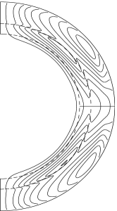
Since we have values of at the ends of cycles 20–23, our procedure for generating a forecast for cycle 24 is now straightforward. We take a relaxed solution of our dynamo code which has been stopped at a solar minimum. We identify this minimum as the minimum at the end of cycle of 20 and change the the values of above in accordance with the value of (which is 1.25). Then we run the code till the next minimum and again change the values of above . Doing this thrice, we come to the minimum at the end of the cycle 23. The next run after this generates the forecast for cycle 24. It may be noted that the poloidal field lines become somewhat discontinuous at after we change the values of above in accordance with observational data. This discontinuity can be seen in Fig. 1 where we plot the poloidal field lines at the minimum before cycle 24 just after updating the values of . However, we find that this discontinuity gets smoothed out within a time scale of weeks.

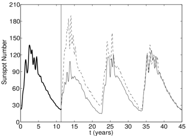
Before presenting results obtained with actual observed values of DM fed into the code, we present some results obtained by changing the poloidal field arbitrarily during a solar minimum and then running the code without any further interruptions. Fig. 2 gives sunspot number plots obtained by increasing and decreasing the poloidal field by 30% above at a solar minimum. We find that the next two solar minima are both affected, after which the memory of the poloidal field change seems to get lost. Svalgaard et al. [3] suggest a simple relation that the maximum International Sunspot Number of cycle will be proportional to the value of DM at the end of cycle , i.e.
On the basis of our model, we expect a more complicated functional relationship
As we shall see below, the results of our dynamo run for the last few cycles are in qualitative agreement with what would be expected from (1). However, if values of DM during the two previous minima are widely different, it is in principle possible that our method based on our dynamo model would generate a forecast for the next cycle significantly different from what is expected from (1).


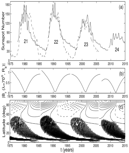
Fig. 3 now presents our results for cycles 21–24 generated by our methodology. The top panel superposes the sunspot number generated from our model on the observational data. The middle panel gives the at a latitude of 70∘ obtained from the dynamo model, showing the jumps at the solar minima when we change the poloidal field in accordance with the observed value of DM. The bottom panel shows the butterfly diagram produced by our model. We see in the top panel that the theoretical plot is in quite good agreement with the observational data for cycles 21–23. whereas cycle 24 comes out as the weakest cycle in a long time. Since the value of DM during the minima at the ends of cycles 22 and 23 are lower than the values of DM in the two preceding minima, the weakness of cycle 24 appears like a very robust result, which does not change with small changes in the parameters of the problem such as the chosen value of . We may point out that the absolute value of the theoretical sunspot number from our numerical code does not have any particular significance, since this value changes on changing such things as the grid spacing. To generate Fig. 3a, we scaled the theoretical sunspot number suitably to make it fit the observational plot.
We are now carrying on calculations in which instead of DM we feed magnetogram data at different latitudes during solar minima into our model. The results will be presented in a future paper. While the use of more detailed polar field data may lead to more realistic predictions, the attractiveness of the scheme presented in this paper is that it is extremely straightforward to implement and is probably reasonably reliable, as we have been able to model cycles 21–23 very well.
Since the dominant processes during the rising phase of a cycle from a minimum to a maximum are fairly regular processes like the magnetic field advection and toroidal field generation by differential rotation, a good knowledge of magnetic configurations during a minimum should enable a good theoretical model to predict the next maximum reliably. On the other hand, the dominant process in the declining phase of a cycle is the poloidal field generation by the Babcock–Leighton process which involves randomness and cannot be predicted in advance by theoretical models. In other words, we suggest that the rising phase of the cycle is predictable (enabling us to predict the strength of the maximum a few years ahead of time), but the declining phase is not predictable. Consequently, it may never be possible to make a realistic prediction of a solar maximum more than 7–8 years ahead of time, even when we have better theoretical models and better magnetic data.
Although our forecast is in agreement with physical intuition as well as forecasts based on polar field strength [3, 4], it is completely opposite of the only other forecast based on a detailed dynamo model [5]. The methodology used by Dikpati & Gilman [5] for feeding the observational data in the theoretical model differs from ours at a fundamental conceptual level. They use the sunspot area as the source term for the generation of the poloidal field, whereas the tacit assumption behind our methodology is that the poloidal field generation involves randomness and cannot be calculated deterministically from the past sunspot data. Cycles with many sunspots do not necessarily produce strong poloidal fields at the end. This is clearly seen in the analysis of Makarov et al. [14] (see their Fig. 1) who have used the positions of H filaments to estimate polar fields for the better part of a century. They find that the polar field during a minimum is correlated with the strength of the next cycle, but the strength of the cycle has no good correlation with the polar field produced at its end. If our identification of the poloidal field generation by the Babcock–Leighton process as the main source of randomness in the solar dynamo is correct, then the methodology of Dikpati & Gilman [5] should in principle not work, although they claim to ‘predict’ many past cycles correctly. Since their forecast for cycle 24 is completely opposite of ours, it should become apparent in the next 4-5 years as to which forecast comes closer to truth.
We thank Dibyendu Nandy, Leif Svalgaard and Jingxiu Wang for discussions. We also express our indebtedness to Dibyendu Nandy for his contributions in developing the code Surya. P. C. acknowledges financial support from Council for Scientific and Industrial Research through grant no. 9/SPM-20/2005-EMR-I. J. J. acknowledges financial support from National Basic Research Program of China through grant no. 2006CB806303.
References
-
[1]
S. Clark, Nature 441, 402 (2006).
-
[2]
K. H. Schatten, P. H. Scherrer, L. Svalgaard, J. M. Wilcox, Geophys. Res. Lett. 5, 411 (1978).
-
[3]
L. Svalgaard, E. W. Cliver, Y. Kamide, Geophys. Res. Lett. 32, L01104 (2005).
-
[4]
K. H. Schatten, Geophys. Res. Lett. 32, L21106 (2005).
-
[5]
M. Dikpati, P. A. Gilman, Astrophys. J., 649, 498–514 (2006).
-
[6]
D. Nandy, A. R. Choudhuri, Science 296, 1671 (2002).
-
[7]
P. Chatterjee, D. Nandy, A. R. Choudhuri, Astron. Astrophys. 427, 1019 (2004).
-
[8]
A. R. Choudhuri, M. Schüssler, M. Dikpati, Astron. Astrophys. 303, L29 (1995).
-
[9]
B. R. Durney, Sol. Phys. 160, 213 (1995).
-
[10]
S. D’Silva, A. R. Choudhuri, Astron. Astrophys. 272, 621 (1993).
-
[11]
D. Longcope, A. R. Choudhuri, Sol. Phys. 205, 63 (2002).
-
[12]
A. R. Choudhuri, The User’s Guide to the Solar Dynamo Code SURYA
(available upon request) (2005).
-
[13]
D. H. Hathaway, R. M. Wilson, Sol. Phys. 224, 5 (2004).
-
[14]
V. I. Makarov, A. G. Tlatov, D. K. Callebaut, V. N. Obridko, B. D. Shelting, Sol. Phys. 198, 409 (2001).