Signal Search and Reconstruction by a Trend Filtering Algorithm

Abstract

We present additional tests of our algorithm aimed at filtering out systematics due to data reduction and instrumental imperfections in time series obtained by ensemble photometry. Signal detection efficiency is demonstrated, and a method of decreasing the false alarm probability is presented. Including the recently discovered transiting extrasolar planet HAT-P-1, we show various examples on the signal reconstruction capability of the method.

Konkoly Observatory, Budapest, Hungary

Harvard-Smithsonian Center for Astrophysics, Cambridge, USA

1. Introduction

One of the most serious challenges in the hunt for transiting extrasolar planets is the removal of the various systematics remaining in the photometric databases even after employing sophisticated methods of CCD image reduction. Sometimes called as “red noise” (Pont, Zucker & Queloz 2006), systematics/trends may show up in many ways. Their most common appearance is a drift with $\sim 1$ d^-1 frequency due to variations of the point-spread function and numerous other parameters, for example focus change, sub-pixel coordinate drifts, etc. In addition to these most trivial systematics, we may have many others, from transients (e.g., imperfect removal of cosmic rays) to periodic saturation of bright stars, depending on Moon phase. During the past several years it has been realized that, except for the simple, high signal-to-noise ratio cases, filtering out these systematics from the databases is absolutely crucial from the point of view of transit search. Therefore, efforts have been taken to devise post processing algorithms that are capable of whitening out the data from the systematics. There are two methods in this field that attracted wider interest. The method SysRem by Tamuz, Mazeh & Zucker (2005) uses basically an iterative principal component analysis to filter out the most prominent systematics from the data. The Trend Filtering Algorithm (TFA) by Kovács, Bakos, & Noyes (2005) is a least-squares method that is capable of filtering out nearly arbitrary systematics, assuming that the selected set of templates is “flavorous” enough, i.e., it contains the light curves necessary for the approximation of the type of trend observed in the target. Here we present tests on the signal recovery capability of TFA.

2. The Algorithm

For completeness, we briefly summarize the basic steps of TFA. First we select a template set of $M$ light curves from the photometric database of the field of interest. From these {$X_{j}(i);j=1,...,M;i=1,...,N$} time series (sampled in $N$ moments of time), we construct the following filter:

$$F(i) = \sum_{j=1}^{M}c_{j}X_{j}(i)\hskip 5.69054pt.$$ (1)

The coefficients {$c_{j}$} for a target {$Y(i)$} are determined by minimizing the following expression:

$$\cal D = \sum_{i=1}^{N}[Y(i)-A(i)-F(i)]^{2}\hskip 5.69054pt.$$ (2)

Here the function $A(i)$ is derived in the following way:

$$A(i)=\left\{\begin{array}[]{ll}\langle Y\rangle=const&\hskip 22.76219pt\mbox{; for period search}\hskip 5.69054pt,\\ A(i)\Leftrightarrow Y(i)-F(i)&\hskip 22.76219pt\mbox{; for signal reconstruction}\hskip 5.69054pt.\end{array}\right.\makebox[65.44133pt][r]{(3)}$$

Namely, in the case of period search we assume that the observed signal is dominated by systematics and noise, and therefore, the filter is expected to yield minimum dispersion around the constant signal average $\langle Y\rangle$. Once the signal is identified, we can recover its shape by iteratively approximating the noiseless and trend-free signal {$A(i)$}. (The iteration is indicated by the symbol $\Leftrightarrow$ in Eq. (3).) In this iterative process we assume that {$A(i)$} can be represented by a low-parameter model, and that the observed signal minus the systematics yield the true signal with white noise.

3. Transit Detection Efficiency

The datasets used in this paper are listed in Table 1. We test transit detection efficiency (TDE), false alarm probability (FAP) and signal reconstruction capability (SRC). For testing SRC on datasets different from those of HATNet (Bakos et al. 2004), we use the HAT-P-1 (Bakos et al. 2006) observations by the 60/90/180cm Schmidt telescope of the Konkoly Observatory.

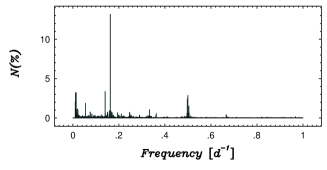
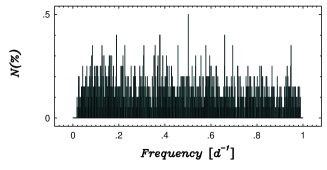
To show that TFA is capable of filtering out nearly all systematics, we compute the distribution function of the peak frequencies obtained by the BLS analysis (Kovács, Zucker & Mazeh 2002). The result of this analysis for field #125 is shown in Fig. 1. We see that the original data includes many stars with various periodic systematics, some of which are not too easy to relate to the daily change of the observational conditions. For example, the strongest peak at $\sim 0.16$ d^-1 is most probably associated with the saturation of the bright stars, because after omitting the first $\sim 400$ stars, the peak at this frequency becomes less prominent than the ones corresponding to other systematics.

Table 1.: Properties of the test datasets

Set	$N$	$N_{\rm star}$	$T$[d]	I [mag]	Purpose
HATnet #125	$6100$	$24980$	$141.0$	$6.3-9.9$	TDE, FAP
HATnet #127	$2100$	$13620$	$167.0$	$7.6-9.7$	FAP
HATnet #148	$5000$	$3430$	$112.0$	$7.4-13.6$	SRC
HAT-P-1, Schmidt	$650$	$202$	$0.32$	$9.6-16.5$	SRC

Notes:    $N$: number of data points per object; $N_{\rm star}$: number of stars in the field; $T$: total time span; I [mag]: I magnitude range in the field.

Figure 1.: : Distribution of the peak frequencies of the BLS spectra of the first 2000 brightest stars in HATNet field #125. Left panel: raw (original) data; right panel: TFAd data with 900 templates. Please note that the application of TFA leads to a nearly flat distribution of the peak frequencies as expected for white noise signals.

We have already demonstrated in Kovács et al. (2005) the ability of TFA of detecting shallow transits that are buried in noise and systematics. Because the statistics we use have slightly changed from then, here we show the results of tests conducted with the new statistics.

We inject a periodic transit signal in the given target from the first $2000$ stars of field #125. Then we run a TFA/BLS analysis on the target and check if the DSP parameter (Kovács & Bakos 2005) corresponding to the highest peak in the frequency spectrum exceeds a given limit. The DSP parameter expresses the significance of the dip corresponding to the transit derived from the analysis. In order to exclude binaries with light reflection and gravitational effects, DSP also includes weighting by the most significant Fourier component of the out-of-transit variation. When computing DSP, we always use the TFA code in the signal reconstruction mode to get a better estimate on this parameter.

Properties of the injected signal and the number of detections are listed in Table 2. We note that the synthetic signal has a flat out-of-transit part and a trapeze shape with rather long ingress/egress durations. The condition of detection is given by a cutoff imposed on DSP. The value of this cutoff is large enough to eliminate false alarms (see Sect. 4). We see that there is a highly significant increase in the detection probability due to the application of TFA. This increase is especially striking when the top 500 bright stars are tested. These are the ones that are most seriously affected by systematics related to saturation effects (see above). We note that the detection ratio can be slightly increased (from $46$% to $50$%) if we choose templates only from this brighter set of stars.

Table 2.: Detection of injected transit signals in field #125

TFA	$N_{\rm star}$	$N_{\rm d}$	$N_{\rm d}$[%]
0	$2000$	$972$	$49$
1	$2000$	$1340$	$67$
0	$500$	$51$	$10$
1	$500$	$228$	$46$

Notes:    Analysis: BLS, with minimum transit duration of $0.01P_{\rm{test}}$, $P_{\rm{test}}\in[1.0,100.0]$ d; Detection condition: DSP$>8.0$; Injected signal parameters: period, $P=5.123$ d; fractional transit length, $q_{\rm tran}=\Delta t_{\rm tran}/P=0.02$; fractional ingress length, $q_{\rm ingr}=\Delta t_{\rm ingr}/\Delta t_{\rm tran}=0.40$; transit depth, $d=-0.015$ mag.

4. False Alarms

By “false alarms” we mean those cases when the detection statistics indicate the presence of a signal, but the probability distribution of the statistics (derived on pure noise) shows that the observed value may also occur due to a random event and the probability of this to happen is “greater than we would like to”. In assessing FAP we resort to direct statistical tests, in which we generate pure Gaussian time series on the time base of the observed light curves. We analyze these artificial time series and count the number of cases when DSP exceeds a prescribed limit. In this way we get estimates on FAPs for a given dataset when TFA and BLS are used.

The results of the tests are presented in Table 3. Several conclusions can be drawn from this table. First of all, as expected, application of TFA introduces correlation in the time series. This increases FAP by a substantial amount. Second, larger number of data points results in a decrease of FAP. Third, larger number of templates leads to stronger correlation, and therefore, to an increase of FAP. Fourth, although increasing the number of data points decreases FAP, it is present in a relative high value even for higher DSP cutoff values (when we already expect a visible sign of the (fake) transit in the folded/binned light curve.

In an attempt to reduce FAP, the following method is suggested. By using several TFA runs, corresponding to various template numbers, we compute DSP values for the given database. Due to the way the template sets are constructed, these results are expected to be largely independent from each other. In a conservative approach of signal detection, we require the signal to be present in all these runs. In the primary selection of transit candidates we require only that the dip is negative (i.e., corresponding to dimming) and that ${\rm DSP}>{\rm DSP}_{\rm cut}$. The result of this multiple template FAP filtering is shown in the lower three lines of Table 3. We see that the method is very effective already with three different TFA runs. For example, even for the sparsely sampled field #127, with three or more different TFA runs we can filter out false alarms with a probability better than 99.9% for signals with DSP$>7$.

Table 3.: Testing false alarms in fields #125 and #127

TFA	$N_{\rm d}(\#127)$				$N_{\rm d}(\#125)$
${\rm DSP}_{\rm cut}$ :	5	6	7		5	6	7
$\emptyset$	68	7	0		26	3	1
a	827	400	107		258	24	2
b	856	523	168		306	31	6
c	842	560	220		394	42	3
d	890	638	328		474	60	5
ab	386	112	9		73	2	0
abc	184	38	1		25	0	0
abcd	97	21	1		14	0	0

Notes:    Test signal: pure Gaussian noise; datasets: the top $2000$ bright stars in each field; Analysis: BLS, with minimum transit duration of $0.02P_{\rm{test}}$, $P_{\rm{test}}\in[1.0,100.0]$ d; TFA template numbers: 0, 700, 800, 900 and 1000 for $\emptyset$, a, b, c and d, respectively; DSP lower detection limits: 5, 6 and 7; Items in the table show the number of detections (negative dips with ${\rm DSP}\geq{\rm DSP}_{\rm cut}$); ab, abc, abcd: datasets used for finding simultaneous detections.

5. Signal reconstruction

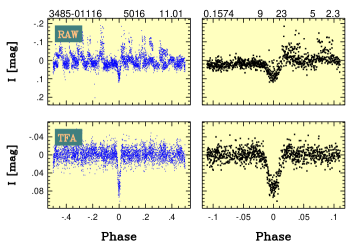
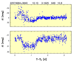
Signal reconstruction is an essential (but optional) part of signal processing when TFA is used. This is because we do not know a priori which part of the observed signal comes from the systematics and which one from the true signal (and all these are coupled with noise). Without knowing the signal parameters a priori, we resort to an iterative scheme in reconstructing the true signal (see also Sect. 2). Our experiments on the HATNet database show that this reconstruction can be quite successful without making any assumption on the signal shape. Once the signal shape is reliably identified, one can proceed by more specific assumptions, e.g., by using trapeze transit shapes, and thereby further decreasing the number of parameters fitted. To illustrate the efficiency of the TFA reconstruction, we show two examples in Fig. 2.

Figure 2.: : Upper panels: ensemble photometry of an eclipsing variable in field #148 (left) and that of HAT-P-1 (right); lower panels: TFA-reconstructed light curves of the same objects. Headers (from left to right): star ID, number of data points, average I magnitude, main BLS frequency [d^-1], signal-to-noise ratio (SNR) of the BLS spectrum, DSP, SNR of the out-of-transit variation and its peak frequency in the units of the BLS frequency. On the right we have: star ID, average magnitude, plotting frequency [d^-1], number of data points, DSP. The reconstruction of HAT-P-1 was made without using its nearby companion star ADS16402 A. In both cases no assumptions were made on the signal shape.

6. Conclusions

Filtering out systematics from astrophysical time series is nearly mandatory if a survey-type analysis is made with the goal of reaching the theoretical white noise limit of signal detection. In the search for extrasolar transiting planets this issue becomes even more highlighted due to the delicacy of the detection. We have shown in this paper that TFA is capable of filtering out various systematics, thereby allowing the detection and a concomitant reconstruction of faint regular (e.g., simple- or multi-periodic) signals. Furthermore, by requiring multiple detections in time series filtered by various TFA templates, false alarm probability can be pushed down near to the white noise limit.

Acknowledgments.

Support for program number HST-HF-01170.01-A to G. Á. B. was provided by NASA through a Hubble Fellowship grant from the Space Telescope Science Institute. Operation of the HATNet project is funded in part by NASA grant NNG04GN74G. We also acknowledge OTKA K-60750.

References

- Bakos et al. (2004) Bakos, G. Á., Noyes, R. W., Kovács, G., et al. 2004, PASP, 116, 266
- Bakos et al. (2006) Bakos, G. Á., Noyes, R. W., Kovács, G., et al., 2006, ApJ, (in press), (astro-ph/0609369)
- Kovács & Bakos (2005) Kovács, G. & Bakos, G. Á. 2005, poster paper (astro-ph/0508081)
- Kovács, Bakos, & Noyes (2005) Kovács, G., Bakos, G. Á., & Noyes, R. W. 2005, MNRAS, 356, 557
- Kovács, Zucker & Mazeh (2002) Kovács, G., Zucker, S. & Mazeh, T. 2002, A&A, 391, 369
- Kruszewski & Semeniuk (2003) Kruszewski A., Semeniuk I. 2003, Acta Astr., 53, 241
- Pont, Zucker & Queloz (2006) Pont, F., Zucker, S., & Queloz, D. 2006, MNRAS, 373, 231
- Tamuz, Mazeh & Zucker (2005) Tamuz, O., Mazeh, T., & Zucker 2005, MNRAS, 356, 1466