Object detection in multi-epoch data

Abstract

In astronomy multiple images are frequently obtained at the same position of the sky for follow-up co-addition as it helps one go deeper and look for fainter objects. With large scale panchromatic synoptic surveys becoming more common, image co-addition has become even more necessary as new observations start to get compared with co-added fiducial sky in real time. The standard co-addition techniques have included straight averages, variance weighted averages, medians etc. A more sophisticated nonlinear response chi-square method is also used when it is known that the data are background noise limited and the point spread function is homogenized in all channels. A more robust object detection technique capable of detecting faint sources, even those not seen at all epochs which will normally be smoothed out in traditional methods, is described. The analysis at each pixel level is based on a formula similar to Mahalanobis distance. The method does not depend on the point spread function.

url]www.stat.psu.edu/$\sim$babu ,

1 Introduction

Many major projects, ongoing and future synoptic surveys, MACHO, OGLE, Palomar-QUEST, Pan-STARRS and LSST, involve repeated scans of large areas of the sky in several spectral bands. Thus an important area of recent astronomical research has been the investigation of source detection in multi-epoch data. A question frequently asked is: What is the best way to combine image regions with low signal to detect faint objects? Historically two basic methods have been used to search for faint astronomical objects:

1. Use a larger telescope to collect a larger number of photons

2. Stack a large number of registered images in order to improve the signal-to-noise ratio.

The former has engineering and monetary limitations while the later may not work for transients that are seen only once and for very faint objects where the signal remains below detection threshold even after the pixel-to-pixel coadding of several images. Szalay et al. (1999) had proposed a method that used chi-square coaddition by treating adjacent pixels to be uncorrelated. It is an improvement over standard coaddition, but since the pixels are in fact correlated, it has its own limitations. The procedure described here is a more robust technique to detect faint sources from multi-epoch data. It is designed not only to have high sensitivity, but to detect changes between images.

The analysis at each pixel level is based on a statistic similar to the measure of distance introduced a by P. C. Mahalanobis in 1936 (Johnson & Wichern 1992, and Atkinson et al. 2004). The Mahalanobis distance $D_{M}$ from a group of values with mean vector $\nu$ and covariance matrix $\Lambda$ from a multivariate vector x is defined as

$$D_{M}({\bf x})=\sqrt{({\bf x}-\nu)\Lambda^{-1}({\bf x}-\nu)^{T}}.$$

It is used in classical multivariate analysis and differs from Euclidean distance. It is scale-invariant, and is based on correlations between variables by which different patterns can be identified and analyzed. Mahalanobis distance can also be defined as dissimilarity measure

$$d_{m}({\bf X},{\bf Y})=\sqrt{({\bf X}-{\bf Y})\Lambda^{-1}({\bf X}-{\bf Y})^{T}}$$

between two random vectors X and Y of the same distribution with covariance matrix $\Lambda$. If the covariance matrix is identity matrix, then the Mahalanobis distance reduces to the Euclidean distance. It is a useful way of determining similarity of an unknown sample set to a known one (Banks et al. 2004, and Atkinson et al. 2004). Mahalanobis distance is available in R Stats package.

The method does not depend on the point spread function, requiring only that the pixel size is invariant. In the following sections we provide the details of the method as well as the tests we have run so far and future plans for large scale implementation.

2 Methodology

We start with $N$ images of a given region of the sky. We first use standard techniques to ensure that all images are the same size in terms of area covered as well as the pixel dimensions. The images are also background subtracted so the mean value in empty parts of each image is close to zero. Suppose the pixel dimensions of each of the images is $(m,n)$. So there are $R$ pixels in each of the image ($=m\times n$). We concentrate on a single pixel $r$. Let f${}^{r}=(f^{r}_{1},\dots,f^{r}_{N})$ denote the row vector of photon counts in $N$ images at pixel $r$. We assume that f^r is approximately Gaussian, i.e.

$${\bf f}^{r}\sim MVN({\bf M},\Sigma),$$

M$=(\mu_{1},\dots,\mu_{N})$ is the vector of means and $\Sigma$ is the variance-covariance matrix. Then ${\bf X}=({\bf f}^{r}-{\bf M})\Sigma^{-1}({\bf f}^{r}-{\bf M})^{T}$ has approximately $\chi^{2}$ distribution. Since approximations are involved, use of bootstrap method, instead of using $\chi^{2}$ tables, to find the critical values (thresholds) at various significance levels is better. Bootstrapping such quadratic forms require special care, see Babu (1984) for details.

This method takes into account potential information in different wave bands. The probability of detecting a source when ${\bf X}>y$ can be obtained from $\chi^{2}$ tables. This incorporates potential correlations of background in different images. If the $f^{r}_{i}$ are all uncorrelated, then the off-diagonal entries of $\Sigma$ are all zero.

Means and covariances can be estimated in two different ways. If the background $M_{i}$ is spatially constant in the i-th image, the covariance matrix $\Sigma$ has entries $s_{i,k}=(1/R)\sum(f^{r}_{i}-M_{i})(f^{r}_{k}-M_{k})$ where $R$ is the number of pixels in each image or cutout. Now the $i,k$-th entry of covariance matrix $\Sigma$ is $s_{i,k}$. This is applicable if the background is similar throughout the image. For spatially variable background, we currently use 9 pixels (the pixel under question and its 8 neighbors) to estimate the covariance matrix $\Sigma(r)$ and the mean vector $M(r)$. If there is no source at pixel r, then $(f^{r}-M(r))\Sigma(r)^{-1}(f^{r}-M(r))^{T}$ has approximately chi-square distribution.

Standard programs like sextractor (SourceExtractor, available from http://terapix.iap.fr) look for a connected set of pixels above a threshold resulting in a list of astronomical objects (called catalog in astronomy jargon) with various flags indicating its validity as an astronomical object based on prior knowledge like that of shapes and profiles of objects built in to the program.

While this technique may not do any better than usual methods for bright objects, under lower signal conditions it is expected to strongly outperform the traditional methods. We will extensively test our technique on the already available PQ (Palomar-QUEST) data in readiness for the even larger stream of LSST data.

As we are testing multiple hypotheses, we need to avoid too many false positives. When there are large number of pixels above the threshold, there may as well be too many falsely discovered source pixels. The proportion of falsely discovered source pixels should be kept to a minimum with any source detection algorithm. The method introduced by Benjamini & Hochberg (1995) (see also Benjamini & Hochberg 1997, and Benjamini & Yekutieli 2005), called False Discovery Rate (FDR) does precisely this, controlling the proportion of incorrectly rejected null hypotheses. T he method allows a priori specification of proportion of false discoveries to total discoveries, and the procedure is independent of the source distribution. An implementation of this procedure is discussed in Hopkins et al. (2002). However, in the examples discussed in the current article, as the detected sources are few and far apart, we shall consider FDR implementation for our method elsewhere. Babu (2004) developed results on bootstrapped empirical process that are relevant in the study of FDR problems.

So far we modeled based on Gaussian assumptions, where least squares methods and maximum likelihood methods coincide. Further, the dependency of pixel data across different filters can be modeled and analyzed with minimum difficulty through covariances and joint multivariate distributions. For Poisson data, modeling the multi-dimensional data with statistical dependence structure is far from clear. Instead it is more natural to consider modeling functional dependency of Poisson rates across filters. This w ill be discussed in a later article.

3 Tests

We carried out a series of tests using artificial data as well as B R I images from the Palomar-QUEST survey (http://palquest.org/). For the former we did the following tests:

1. artificial data with zero background and no noise added,

2. artificial data with non-zero constant background, but no noise,

3. artificial data with non-zero constant background and corresponding Poisson noise added.

We found that our method could recover all objects that the standard coadding gets, and then some. It fails if two or more objects are blended such that they overlap by a large fraction.

For real data we obtained cutouts (image subsections) of size 60’ x 2’ for a few pointings on the sky at several different epochs. Individual CCDs on Palomar-QUEST are about 8’ wide. The dithering strategy followed for the survey necessitates choosing such narrow strips to ensure that for the different scans we do not straddle different CCDs.

Figure 1: $B$ band images of a small portion of the sky from the Palomar-QUEST multi-epoch survey. The three panels show co-adds from 3 (top), 5 (middle) and 7 (bottom) epochs. The images on the left are formed by a traditional pixel-by-pixel averaging procedure (mean after rejection of minimum and maximum points) with4$\sigma$ sources circled. The images on the right are formed by the statistic based on Mahalanobis distance with 4$\sigma$ sources circled.

(This does not mean that we can not do larger areas. It is just that for current exploratory investigations we wish to keep inter-CCD calibrations out of the picture). The images were coadded in the standard way as well as using our method. Object catalogs were then obtained for both sets at a series of significance levels.

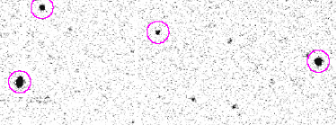
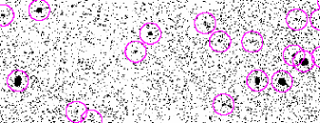
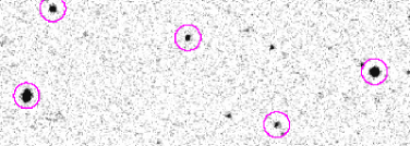
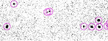
The results there too have been good. We coadded 3, 5 and 7 images using both methods and found that our method does almost as well as the traditional method in most cases and better in many others. This has been quantified with a few tests and tabulated, but more stringent tests are needed for large scale use. An example is to change the number of neighboring pixels considered to constitute the correlation matrix.

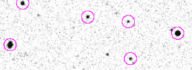
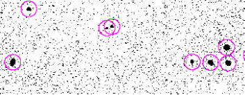
Some preliminary results based on Palomar-Quest images are shown in Figure 1. Our images are more grainy in appearance than the traditional co-added images due to the removal of correlation between adjacent pixels. When more image layers are added, the graininess decreases. The emergence of 3 (two in the top right panel) objects, in line at the bottom right corner of the lower panels of the three images, absent in the left panels is likely due to the passage of a minor planetary body (asteroid, Kuiper Belt Object) through the field.

4 Other possibilities

Figure 2: An example of high-redshift quasar selection, as outliers in a color-color parameter space, from a small area covered in the PQ survey. Normal stars (dots) form a well-defined locus in this parameter space; quasar candidates (solid circles) deviate from this locus, while having exactly the same unresolved image morphology as the stars.

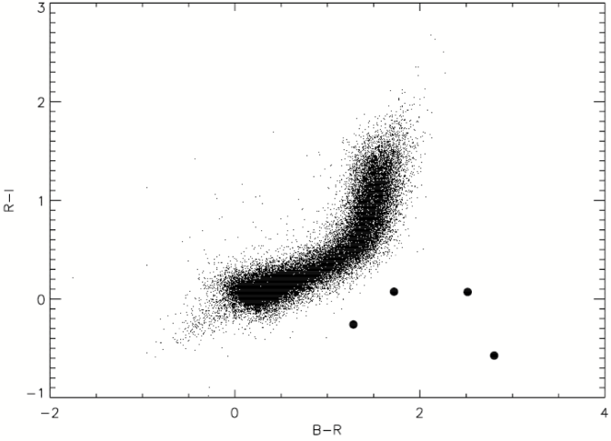
In addition to source detection, a related problem that can be addressed with this technique is that of identifying faint objects in a particular region of color-color space. A color indicates the ratio of fluxes in two bands. A color-color diagram then is a plot which has such ratios formed from 3 bands: A/B on x-axis, and B/C on y-axis. An example color-color diagram depicting $B-R$ and $R-I$ colors from Palomar-QUEST is seen in Figure 2. Objects of a given type occupy particular sections of this plot. Thus for an area of interest e.g. one that is expected to contain hi-z quasars, one could try: $(f_{k}-f_{i})*a*(f_{i}-f_{z})$. This can be tested by populating different colored objects and trying detection in single band, combined bands and using the above technique. Standard squaring as is used in calculating Euclidean distances may have to be avoided as sign of the color is important. For bright normal images this technique may not do well, but under lower signal conditions it is expected to perform better.

5 Future work

As we refine the method for large data sets, we are starting to incorporate it in to the Palomar-QUEST real-time pipeline. Initially some handholding will be needed as Palomar-QUEST images in each of four filters for a given night is about 1500 times the size of the test images tried so far. The advantage will be to be able to see fainter objects and hence curb the rate of false alerts for transients. The methodology will also set a standard for the forthcoming synoptic surveys like Pan-STARRS and LSST can reap rich benefits thereof.

References

- [1] Atkinson, A. C.; Riani, M.; and Cerioli, A. (2004). Exploring multivariate data with the forward search. Springer Series in Statistics. Springer-Verlag, New York.
- [2] Babu, G. J. (1984). Bootstrapping statistics with linear combinations of chi-squares as weak limit. Sankhyā, Series A, 46, 85–93.
- [3] Babu, G. J., 2004. A note on the bootstrapped empirical process. J. of Statistical Planning and Inference, 126, no. 2, 587–589.
- [4] Banks, D.; House, L.; McMorris, F. R.; Arabie, P.; and Gaul, W. (Editors). (2004). Classification, clustering, and data mining applications. Proceedings of the Meeting of the International Federation of Classification Societies held at the Illinois Institute of Technology, Chicago, IL, July 15–18, 2004. Studies in Classification, Data Analysis, and Knowledge Organization. Springer-Verlag, Berlin.
- [5] Benjamini, Y.; and Hochberg Y. (1995). Controlling the false discovery rate: a practical and powerful approach to multiple testing. Journal of the Royal Statistical Society, Series B 57, 289–300.
- [6] Benjamini, Y.; and Hochberg, Y. (1997). Multiple hypotheses testing with weights. Scand. J. Statist., 24, no. 3, 407–418.
- [7] Benjamini, Y.; and Yekutieli, D. (2005). False discovery rate-adjusted multiple confidence intervals for selected parameters. With comments and a rejoinder by the authors. J. Amer. Statist. Assoc., 100, no. 469, 71–93.
- [8] Hopkins, A. M.; Miller, C. J.; Connolly, A. J.; Genovese, C.; Nichol, R. C.; and Wasserman, L. (2002). A new source detection algorithm using the false-discovery rate. AJ, 123, 1086–1094.
- [9] Johnson, R. A.; and Wichern, D. W. (1992). Applied multivariate statistical analysis. Third edition. Prentice Hall, Inc., Englewood Cliffs, NJ.
- [10] Szalay, A. S., Connolly, A. J., and Szokoly, G. P., 1999. Simultaneous Multicolor Detection of Faint Galaxies in the Hubble Deep Field. AJ, 117, 68–74.