The velocity field of the local universe from measurements of type Ia supernovae
Abstract
We present a measurement of the velocity flow of the local universe relative to the CMB rest frame, based on the Jha, Riess & Kirshner (2007) sample of 133 low redshift type Ia supernovae. At a depth of 4500 we find a dipole amplitude of in the direction , , consistent with earlier measurements and with the assumption that the local velocity field is dominated by the Great Attractor region. At a larger depth of 5900 we find a shift in the dipole direction towards the Shapley concentration. We also present the first measurement of the quadrupole term in the local velocity flow at these depths. Finally, we have performed detailed studies based on N-body simulations of the expected precision with which the lowest multipoles in the velocity field can be measured out to redshifts of order 0.1. Our mock catalogues are in good agreement with current observations, and demonstrate that our results are robust with respect to assumptions about the influence of local environment on the type Ia supernova rate.
1. Introduction
Distant type Ia supernovae (SNe Ia) have been used to probe the expansion rate of the Universe out to redshifts of order 1.5 (see e.g. Riess et al., 2004). These measurements were crucial in establishing the current standard model of cosmology in which roughly 30% of the energy density is in the form of non-relativistic matter, whereas roughly 70% is in the form of a dark energy, a component with negative pressure.
The power of supernova surveys as cosmological probes depends on a precise measurement of the luminosity distance to the individual supernovae - but the supernova host galaxies do not follow the Hubble flow. They have peculiar velocities, induced by the underlying gravitational potential, and the measured luminosity distances and redshifts are perturbed in correlation with the large scale structure (see e.g. Miller & Branch, 1992).
The measured fluctuations in the luminosity distances from nearby supernovae surveys can be related to the local variation in the Hubble parameter (Riess et al., 1995), and the local large scale structure, and can be quantified in terms of their correlation functions. This possibility has been studied in several recent papers (Bonvin et al., 2006a, b; Hui & Greene, 2006) (see also Sugiura, Sugiyama & Sasaki, 1999) using analytical methods. Bonvin et al. (2006b) detected the dipole term with respect to the CMB at roughly 2 confidence. The variation of the monopole contribution with redshift was studied by Zehavi et al. (1998) using the same supernova sample as (Riess et al., 1995).
In contrast to measurements of the density field, velocity field measurements are much less sensitive to selection bias, since the field is measured directly instead of summed up from number counting, but it is very sensitive to uncertainties in the measured luminosity distance. Because of this type Ia supernovae are particularly useful as probes of the velocity field because of the very small inherent uncertainty in their luminosity distance. Compared with measurements using galaxies as standard candles much fewer supernovae are needed to get a reliable estimate of at least the lowest multipoles in the velocity field.
The purpose of the present paper is twofold. The first is to perform a theoretical study of the problem of extracting the velocity field from supernova data. The second is to use the developed formalism on the best available data set to extract precise values of the dipole and quadrupole terms in the local velocity field.
We first use large scale dark matter N-body models to predict the observed angular power spectrum of the peculiar radial velocity field as a function of redshift and to explore its utility to probe the local velocity field. By using this method we are able to quantify the effect of various error sources as well as cosmic variance.
We also use the Jha, Riess & Kirshner (2007) (hereafter JRK) sample of nearby type Ia supernovae to calculate the lowest multipoles of the local velocity field. We find that both the dipole and the quadrupole terms are well measured by this sample. Higher multipoles cannot be reliably estimated with the JRK sample because of sparse sampling. In Jha et al. (2007) this sample was also used to probe the monopole term in an analysis similar to that of Zehavi et al. (1998). Similar evidence of a local void was found in Jha, Riess & Kirshner (2007), even taking a data set which is completely disjoint from that in Zehavi et al. (1998). In the following we will concentrate on the dipole and quadrupole terms in the JRK sample since the monopole has already been exhaustively discussed in Jha et al. (2007).
In Section 2 we discuss the formalism used to derive the velocity field from magnitude measurements. In Section 3 we present the analysis tools used to extract the multipole components of the velocity field from a finite sample of supernovae. In Section 4 we use catalogues from N-body simulations to study the expected properties of the velocity field, including the precision with which it can be probed by supernova surveys. We apply the same formalism to the JRK sample and provide a detailed discussion of the results in Section 5. Finally, Section 6 contains a comparison with other measurements of the local velocity field, and in Section 7 we provide our conclusions.
In the following we will take .
2. Distance measures and radial velocities
The luminosity distance, , to a supernova at redshift is given by the definition
| (1) |
where is the observed flux and the luminosity, or equivalently by
| (2) |
where is the apparent and the absolute magnitude. The angular-diameter distance, , to the same supernova is defined as
| (3) |
In a homogeneous and isotropic universe the two distance measures, and , are given by
| (4) |
where
| (5) |
By taking the logarithmic derivative of Eq. (4) with respect to in the special case of a flat universe () we obtain
| (6) |
where
| (7) |
However, in a perturbed universe, the luminosity distance depends on the detailed trajectory of the individual photons from the supernova to the observer. At moderately high redshifts () the contribution arising from lensing by intervening matter dominates, while at low redshifts () the contribution from the peculiar velocities of the supernova host galaxy relative to the observer dominates. In this paper we are only concerned with the local universe. From now on we will therefore only consider the contribution from the peculiar velocities in determining distances. For a given supernova and observer, each with some peculiar velocity, the measured redshift , angular-diameter distance, , and luminosity distance, , are modified according to (Hui & Greene, 2006; Bonvin et al., 2006b)
| (8) | |||||
| (9) | |||||
| (10) |
where by definition
| (11) | |||||
| (12) |
A bar indicates the quantities as measured in a homogeneous and isotropic cosmology, and is the velocity of the supernova projected along the direction from the observer to the supernova. Having measured the redshift, , and the flux, , of the supernova we can calculate the luminosity distance, , and the angular-diameter distance, , to within a scatter determined by the cosmic variance on the luminosity, , of a supernova. As we know the peculiar velocity, , of the observer with respect to the CMB with great accuracy it is useful to collect all known quantities on the left hand side of the three equations:
| (13) | |||||
| (14) | |||||
| (15) |
The three quantities , , and are the redshift, angular-diameter distance, and luminosity distance as measured and calculated by an observer at rest with respect to the CMB. In the following we assume that the measured quantities all have been corrected to a frame at rest with respect to the CMB. The measured redshift, , is most transparently split into the cosmological redshift, , and the radial velocity of the supernova, , by inverting Eq. (14) to find , which is then inserted into this alternative form of Eq. (13):
| (16) |
It is also possible to begin with Eq. (16) to obtain the cosmological redshift, , in terms of the measured redshift, , and the radial velocity, , of the supernova:
| (17) |
We now expand the natural logarithm of the angular-diameter distance, , to first order around the measured redshift, , and by using Eq. (14) we obtain
| (18) |
where for a flat universe is given by Eq. (6). This equation applies equally well for the luminosity distance, so we can give a common formula for both distance measures:
| (19) |
This expression can easily be transformed into an equation between the measured apparent magnitude, , the calculated apparent magnitude, , at the measured redshift, , and the peculiar radial velocity, , of the supernova:
| (20) |
Inverting this equation for the special case of a flat universe we obtain
| (21) |
For low redshift supernovae the Hubble parameter, the angular-diameter distance, and the luminosity distance can all be expanded in terms of the deceleration parameter, :
| (22) | |||||
| (23) | |||||
| (24) |
When we insert these values into Eq. (21) we obtain the radial velocity of a low redshift supernova
| (25) |
In this approximation the distance modulus, , is given by
| (26) | |||||
where the Hubble constant as usual is given as . The distance modulus defined in Eq. (26) should be compared with the distance modulus, , as measured in a frame at rest with respect to the CMB. The difference between the apparent magnitude and the one measured by the observer, , is according to Eq. (15),
| (27) |
The approximate equation (25) is sufficient for the low redshifts that we are considering, while at higher redshifts one has to use the correct form Eq. (21), and also take into account other contributions to , such as lensing.
3. Analysis using an angular expansion of the radial velocity field
We analyse both the mock catalogues discussed in the next section and the real data set (see section 5) using the same technique. In practice we decompose the field into spherical harmonics.
The radial velocity is a real scalar field, and on a spherical shell of a given redshift it can be decomposed into spherical harmonics
| (28) | |||||
Using for the expansion of a real function and we obtain
However, this applies strictly only if the field can be measured on the entire sphere. In our case the radial velocity field is measured for a finite number of directions, so we can only hope to determine a finite number of coefficients by fitting a truncated multipole expansion by the method of weighted linear least squares using as basis functions. Specifically, we solved the problem by a singular value decomposition.
We follow the procedure by Copi, Huterer, Schwarz, and Starkman (2006) and represent the ’th multipole in terms of a scalar, and unit vectors, :
| (30) |
where , and is the sum of all possible traces of the first term. In this representation the multipole expansion up to and including the quadrupole term takes the following form:
| (31) | |||||
Note that and are “headless” vectors only defining a line, not a direction. Equivalently they define a plane, but they do not define a rotation in that plane, so the normal to the plane is also headless. By convention we choose as the first vector, , the one with the largest absolute z-coordinate. We can choose to point to the hemisphere near the pole without introducing a negative amplitude , if both and have their sign changed. Finally we define the normal to the plane spanned by the two vectors as . This is the polar quadrupole vector.
From the coefficients the monopole amplitude can be found as
| (32) |
and the dipole amplitude and direction can be found as
| (33) | |||||
| (34) | |||||
| (35) |
This is the direction of the maximum of the dipole. All the higher order multipole vectors are found by using the program mpd_decomp by Copi et al. (2006).
For the lowest -values the amplitudes in the multipole vector expansion are related to the usual power as (Copi et al., 2006)
| (36) | |||||
| (37) | |||||
| (38) |
It should be noted that in general the individual multipole coefficients obtained in the fit to data can be strongly dependent on the number of modes included. The reason for this is that the window function does not cover the entire sky, rather there are patches with zero coverage. This means that the spherical harmonics are no longer orthogonal, and shows up as a leakage of power between different . In fact, this is predicted to be a significant problem for any harmonic analysis with limited sampling because the higher order multipoles do contribute significantly to the rms velocity. In Section 5.1 we discuss the implications of sampling for the JRK sample.
4. Synthetic supernova surveys from Monte Carlo simulations
Before analysing existing data we make mock catalogues of supernova data based on dark matter N-body simulations. This is done in order to get an estimate of the various sources of error in such measurements. The N-body simulations were done using the Gadget-2 code (Springel, 2005; Springel, Yoshida & White, 2000) with a box size of and & particles respectively to make synthetic realisations. The box size is chosen large enough that the periodic nature of the box does not impact the simulation at the scales (, or ) we are interested in, and the high resolution run is made to assure that our results are not dependent on the numerical resolution. In Fig. 1 is shown a typical all sky map in Mollweide projection of the peculiar velocity field at redshifts , computed in the CMB rest frame.
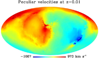
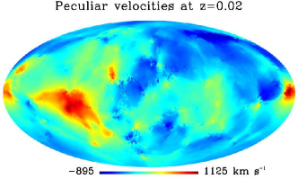
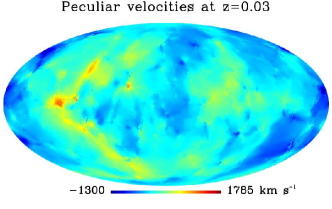
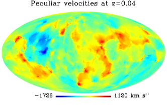
The formation rate of SNe Ia as a function of the environment is not well known, though there are indications that at low redshifts the rate is directly proportional to the stellar mass, and insensitive to the metalicity (Neill et al., 2006) (though see Sharon et al., 2006; Sullivan et al., 2006, and references therein for indications of a bimodal distribution). On the other hand the semi-analytic estimates in the literature (see e.g. Bonvin et al., 2006b; Hui & Greene, 2006) assume a rate which is uniform on the sky. This is clearly not realistic, but to test the effect on the luminosity distance distributions we have made synthetic data sets using both a rate proportional to the mass and an uniform distribution. In Fig. 2 we show the distribution of peculiar radial velocities in the two models. The differences between the two scenarios are at a percent level. Looking at Fig. 1 we see that the radial velocity field is smooth across voids in contrast to e.g. scalar fields like the density field. This is because it is only a pseudo-scalar, and the underlying vector field can be transported efficiently (i.e. it is easier to change the direction of a vector, than transport a scalar quantity).
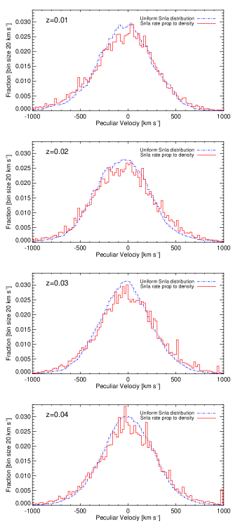
4.1. Making a mock supernova survey
Real measurements rely on a tracer of the matter distribution, whether it is galaxies or SN Ia. In any case, only a finite number of objects will be available. Furthermore there will be a selection bias coming from the presence of galactic foregrounds etc. In this work we generate a mock supernova survey using the following strategy:
a) The total number of measured SNe in a redshift bin, , is chosen.
b) Each SN is generated by sampling one of the two probability distributions described in the previous section.
c) To each SN a noise component is added, resulting from scatter in the (stretch corrected) intrinsic luminosity, uncertainty in extinction correction, measurement errors etc. We describe the errors as a Gaussian error with a spread of on the measured apparent magnitude of the SN.
From this data set the angular power spectrum is calculated. For each type of simulated survey this task is performed 500 times for 27 different observers, to find the mean and variance of the angular power spectrum.
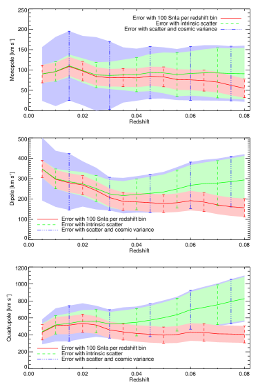
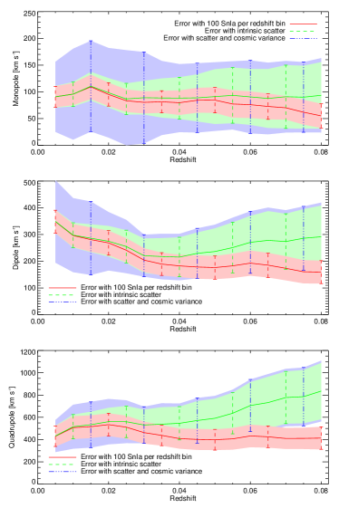
We choose a set of SNe per bin in 16 redshift bins at redshifts of or equivalently with Hubble flow velocities . This conforms roughly to the expectations from local supernova searches conducted today (Li et al., 2003; Krisciunas et al., 2004; Jha et al., 2006) and in the near future (Aldering et al., 2002; Frieman et al., 2004; Hamuy et al., 2006), if they are binned into 3 or 4 redshift bins. In Figs. 3-4 we show the evolution of the lowest multipoles as a function of for both models of the supernova distribution. The red line and error bars show how a hypothetical survey without any external error sources, , would perform. Hence, the error here is only due to the finite number of SNe that are used to probe the velocity field. The green line shows the same, but including a Gaussian scatter of is included. Using the 27 different realisations we can estimate the size of cosmic variance (shaded blue area).
From the figures it is clear that with 100 homogeneous distributed SNe per redshift bin both the dipole and the quadrupole can be measured out to a redshift of about 0.1. Furthermore for the synthetic observations, we know the underlying cosmology and the real Hubble constant, and we can determine the monopole. In the case of real observations we can only measure the relative change. In other words the zero point is in principle only measurable asymptotically at high redshifts. Looking at the red curve, we see that for all multipoles the power goes to zero at higher redshift, as the flow approach the background Hubble flow. We also note that cosmic variance is very large in the monopole term. This indicates that the local “Hubble Bubble” phenomena, such as those found in Zehavi et al. (1998); Jha et al. (2007), are not unlikely.
The velocity amplitudes are positive definite, and including a Gaussian scatter in the velocities, is adding uncorrelated noise to the (synthetic) observations. Therefore the amplitudes of the multipoles, when errors are included, are overestimated. This error is per se hard to separate from the signal, but can trivially be beaten down by a better control of the intrinsic errors or increasing the number of SNe per redshift bin. Given an observational data set synthetic observations with a realistic sky distribution should be used to separate the noise amplitude from the underlying velocity field.
In accordance with the underlying velocity distribution (Fig. 2), on average there is a 5% overestimation of the radial velocity amplitudes, when assuming the Sn Ia rate is proportional to mass compared to a uniform distribution.
5. Results from the JRK sample of nearby supernovae
We apply the analysis technique described in section 3 to the sample of 133 nearby supernovae obtained by JRK. The JRK sample includes 95 type Ia supernovae in the Hubble flow, with an intrinsic dispersion of less than in distances. This is the best sample available with distances derived in a homogeneous way, by using the Multicolor Light Curve Shape (MLCS2k2) method described in Jha et al. (2007). This method is one of several others used to standardise supernova distances, but is particularly powerful in that it allows a disentangled correction for host galaxy extinction and also provides a statistically reliable way to estimate the errors.
The entire JRK sample comprises 133 supernovae. We have selected 3 sub samples of these for our analysis. We followed Jha et al. (2007) in selecting as the first sub sample 95 Hubble flow supernovae, the HF sample, a selection based on distance cut, requirement of an acceptable light curve fit and excluding objects with very high extinction. The SNe in this sample have redshifts between and and a weighted average redshift of or . The second sub sample, the 4500 sample, includes 74 SNe, and is similar to the HF sample, but without the highest redshift SNe and including a few SNe with a lower redshift. It has an weighted average of or and contains SNe with redshift between 0.007 and 0.035. The last sub sample, the 3500 sample, includes 42 SNe, and is similar to the 4500 sample, but without the highest redshift SNe. It has an weighted average of or and contains SNe with redshift between 0.007 and 0.017.
To the uncertainties in the distance moduli, we also add in quadrature an additional error of 0.08 mag in order to properly represent the final uncertainties following Jha et al. (2007). In addition we add in quadrature to the errors in the radial velocity in order to take the velocity dispersion around the local anisotropic Hubble flow into account. Karachentsev et al. (2003) find that the radial velocity dispersion around the local (anisotropic) Hubble flow within Mpc amounts to only , when distance errors are taken into account. For further details on the samples we refer to Jha et al. (2007).
5.1. The effective window function
In Fig. 9 we show the distance to the nearest supernova on the sky, measured in degrees, for all points on the sphere.
The sample has good coverage, except for a few “holes” mainly defined by the galactic disk. The mean distance to the nearest supernova is , but the maximum distance is at , . There are three areas with distance larger than , roughly centred on , and respectively. For a given , the distance between zero points in the field is . If the largest holes in the sample have a size of then the multipole decomposition becomes problematic around . For the present sample this corresponds to so that the quadrupole can be robustly fitted, but not the octupole. We have tested this in practice. When the quadrupole is added, the monopole and dipole amplitudes and the dipole direction hardly change. However, when the octupole is included there is serious leakage of power from the lower ’s to and the results change substantially. The reason is that the fit in the well-sampled regions can be improved by adding the additional 7 coefficients to the fit, but that this happens at the expense of very large changes in the unsampled regions. In order to probe the higher order multipoles it is essential to reduce the size of the voids in the sample. For a uniformly distributed sample of 95 supernovae the average distance to the nearest supernova is 10.4 degrees, nearly the same as in the JRK sample. However, the average maximum distance is 30.1 degrees, significantly lower than in our sample. A uniform sample of 95 supernovae could be used to probe robustly. For a uniform sample the average distance to the nearest supernova scales as , and the average maximum distance in the sample roughly as .
5.2. Results
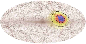
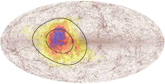
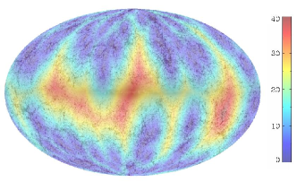
In Figs. 6-8 we show the obtained 68% and 95% contours for the direction of the dipole and quadrupole vectors in galactic coordinates. The corresponding best fit values with their formal 68% errors are shown in Tables 1 and 2.
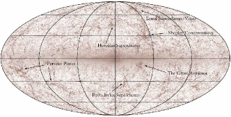
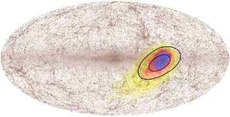
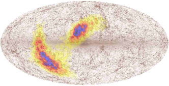
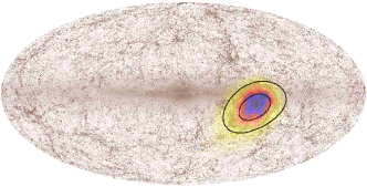
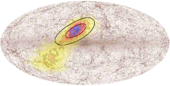


This result can be compared to other velocity surveys based on galaxy samples. The recent review by Feldman, Sarkar & Watkins (2006) summarises these surveys. At an effective depth of 4000 they find that the dipole amplitude is in direction and .
5.2.1 Dipole
The 3500 and 4500 samples both show a dipole in a direction compatible with the Great Attractor region at , . For the HF sample the direction shifts to slightly higher , compatible with a shift in the motion towards the Shapley concentration (which lies at an average distance of 14000 , Bardelli et al., 1994) at slightly higher galactic latitude. Furthermore the amplitude of the dipole decreases, as is expected from the Monte Carlo simulations.
5.2.2 Quadrupole
For all the three sub samples we find a relatively large contribution from the quadrupole, showing that the local flow has a significant shear component. The result is consistent in magnitude with the expectation from the Monte Carlo simulations. From the figures it can also be seen that there is a change in quadrupole direction with redshift, and that the distributions for the 3500 and 4500 samples are bimodal. This could be because the quadrupole is pointing in different directions at the lower and higher end of the included redshift range of the SNe, and hence for the 3500 sample the bimodality is more apparent. Even though we quote formal 68% errors in Table 2 the distribution is highly non-Gaussian and the error bars should be taken as indicative only.
| Sample | |||
|---|---|---|---|
| 3500 | |||
| 4500 | |||
| HF |
| Sample | |||
|---|---|---|---|
| 3500 | |||
| 4500 | |||
| HF |
6. Comparison with other results
6.1. SNIa
The Tonry et al. (2003) data set of 98 SNe was analysed by Hudson et al. (2004) in order to find the local dipole. For the part of the sample with they found a dipole of towards , . They do not quote error bars on this result, but for the part of the sample with the stated errors are for and for . This result is completely compatible with our result for the dipole. However, Hudson et al. quote no results for the higher order terms.
Jha et al. (2007) also provide a crude estimate of the dipole amplitude and direction from a subset of 69 supernovae in their sample which is roughly compatible with our 4500 sample . In the coordinate system of the Local Group they find a velocity of towards a direction of . If we transform our dipole term from the HF sample to the same coordinate system, using the Local Group velocity derived in Rauzy & Gurzadyan (1998), we find a velocity of towards . Both the amplitude and direction are compatible with the JRK value at 1. Our derived amplitude is slightly lower (although not significantly so), because in our fit the quadrupole term accounts for part of the velocity.
As noted before, we do not discuss the local monopole term. By subdividing supernovae into low and high redshift bins (Zehavi et al., 1998; Jha et al., 2007), a significant variation in the local Hubble parameter has been detected. This does not have any impact on our results (see section 5.1), and since it was discussed thoroughly in Jha et al. (2007) we refer to that paper for further details.
6.2. Galaxy surveys
Results from galaxy velocity surveys on scales of order 4000-6000 generally agree that the magnitude of the dipole is of order 300 in the direction , (see for instance Zaroubi (2002) and references therein). This result is compatible with the SN Ia dipole direction and magnitude within .
A reconstruction of the very local velocity field () was done by Tonry et al. (2000) measuring surface brightness fluctuations in 300 early type galaxies, predominantly in groups and clusters. They used an explicit flow model with a Virgo Attractor and a Great Attractor which contain the main local mass concentrations. Furthermore they added dipole and quadrupole terms to account for the gravitational pull and shear from large scale structure further away. They find a very low value of the dipole () and the quadrupole polar vector (), but it may be related to having the dipole in the same direction as the attractors, and the attractors accounting for the major part of the shear (quadrupole term) in the model.
6.3. Clusters
Cluster samples like SMAC probe larger distances, and find directions which are generally compatible with the SN Ia result. For example Hudson et al. (2004) find , . However, they find an amplitude of , significantly higher than our result (although again compatible at ).
7. Discussion
We have analysed mock supernova surveys in order to study the number of supernovae needed to probe the large scale velocity field of the local universe, quantified in terms of the angular power spectra as a function of redshift. We then proceeded to use the best available database of low-redshift supernovae, the JRK sample, to probe the local dipole and quadrupole of the velocity field at three different distances. The present method has several advantages over galaxy surveys. The uncertainty on each individual supernova luminosity is much smaller than the systematic uncertainties in determining galaxy luminosities so that a much smaller sample is sufficient. We find that
-
•
With two different models for the type Ia supernova rate, the resulting mock surveys only differ at the percent level. Hence, using SN Ia to probe the underlying velocity field is robust with respect to assumptions about the supernova environment.
-
•
For the dipole we find a result which is consistent with galaxy surveys at the same Hubble flow depths.
-
•
The quadrupole is comparable in value to the dipole, indicative of a significant shear in the local velocity field, in accordance with our mock catalogues. It has, to our knowledge, not been measured before at these distances.
-
•
With the present sample size of almost 100 supernovae the precision of the dipole measurement is comparable to that in galaxy surveys using thousands of galaxies.
Finally, we note that new surveys like Pan-STARRs, SkyMapper and LSST will measure about 10,000 type Ia supernovae at per year, and if proper light curves and redshifts can be measured for even a small fraction of these events they will provide an extremely powerful tool for studying the dynamics of the local universe.
Acknowledgements
We thank the Danish Centre of Scientific Computing (DCSC) for granting the computer resources used. TH thanks the DARK Cosmology Centre for hospitality during the course of this work. SJ is grateful for support at KIPAC and SLAC via the Panofsky Fellowship. The Dark Cosmology Centre is funded by the DNRF.
References
- Aldering et al. (2002) Aldering, G., et al. 2002, Proc. SPIE, 4836, 61
- Bardelli et al. (1994) Bardelli, S., et al. 1994, MNRAS, 267, 665
- Bonvin et al. (2006a) Bonvin, C., Durrer, R., & Gasparini, M. A. 2006, Phys. Rev. D, 73, 023523
- Bonvin et al. (2006b) Bonvin, C., Durrer, R., & Kunz, M. 2006, Phys. Rev. Lett., 96, 191302
- Cooray & Caldwell (2006) Cooray, A., & Caldwell, R. R. 2006, Phys. Rev. D, 73, 103002
- Copi et al. (2006) Copi, C. J., Huterer, D., Schwarz, D. J., & Starkman, G. D. 2006, MNRAS, 367, 79
- Erdoğdu et al. (2006a) Erdoğdu, P., et al. 2006, MNRAS, 373, 45
- Erdoğdu et al. (2006b) Erdoğdu, P., et al. 2006, MNRAS, 368, 1515
- Feldman, Sarkar & Watkins (2006) Sarkar, D., Feldman, H. A. & Watkins, R. 2006, astro-ph/0607426
- Frieman et al. (2004) Frieman, J., et al. 2004, BAAS, 36, 1548
- Hamuy et al. (2006) Hamuy, M., et al. 2006, PASP, 118, 2
- Hudson et al. (2004) Hudson, M. J., Smith, R. J., Lucey, J. R., and Branchini, E. 2004, MNRAS, 352, 61
- Hui & Greene (2006) Hui, L., & Greene, P. B. 2006, Phys. Rev. D, 73, 123526
- Jha et al. (2006) Jha, S., et al. 2006, AJ, 131, 527
- Jha et al. (2007) Jha, S., Riess, A. G. , and Kirshner, R. P. 2007, submitted to ApJ
- Karachentsev et al. (2003) Karachentsev, I. D., Makarov, D. I., Sharina, M. E., et al. 2003, A&A, 398, 479
- Krisciunas et al. (2004) Krisciunas, K., et al. 2004, AJ, 128, 3034
- Li et al. (2003) Li, W., et al. 2003, PASP, 115, 453
- Miller & Branch (1992) Miller, D. L. and Branch, D. 1992, AJ, 103, 379
- Neill et al. (2006) Neill, J. D., et al. 2006, AJ, 132, 1126
- Pike & Hudson (2005) Pike, R.W. & Hudson, M. J. 2005, ApJ, 635, 11
- Rauzy & Gurzadyan (1998) Rauzy, S. & Gurzadyan, V. G. 1998, MNRAS, 298, 114
- Riess et al. (1995) Riess, A. G., Press, W. H., & Kirshner, R. P. 1995, ApJ, 445, L91
- Riess et al. (2004) Riess, A. G., Strolger, L.-G., Tonry, J. et al. 2004, ApJ, 607, 665
- Sarkar, Feldman & Watkins (2006) Sarkar, D., Feldman, H. A. and Watkins, R. 2006, arXiv:astro-ph/0607426
- Sharon et al. (2006) Sharon, K. et al. 2006, astro-ph/0610228
- Shi & Turner (1997) Shi, X. D. and Turner, M. S. 1998, ApJ, 493, 519
- Springel (2005) Springel, V. 2005, MNRAS, 364 1105
- Springel, Yoshida & White (2000) Springel, V., Yoshida, N. and White, S. D. M. 2001, New Astron., 6, 79
- Sugiura, Sugiyama & Sasaki (1999) Sugiura, N., Sugiyama, N., & Sasaki, M. 1999, Prog. of Theoretical Physics, 101, 903
- Sullivan et al. (2006) Sullivan, M., et al. 2006, ApJ, 648, 868
- Tonry et al. (2000) Tonry, J. L., Blakeslee, J. P., Ajhar, E. A., & Dressler, A. 2000, ApJ, 530, 625
- Tonry et al. (2003) Tonry, J. L. et al. 2003, ApJ, 594, 1
- Zaroubi (2002) Zaroubi, S. 2002, arXiv:astro-ph/0206052
- Zehavi et al. (1998) Zehavi, I., Riess, A. G., Kirshner, R. P. and Dekel, A. 1998, ApJ, 503, 483