Hints of Isocurvature Perturbations in the Cosmic Microwave Background?

Abstract

The improved data on the cosmic microwave background (CMB) anisotropy allow a better determination of the adiabaticity of the primordial perturbation. Interestingly, we find that recent CMB data seem to favor a contribution of a primordial isocurvature mode where the entropy perturbation is positively correlated with the primordial curvature perturbation and has a large spectral index ($n_{\rm{iso}}\sim 3$). With 4 additional parameters we obtain a better fit to the CMB data by $\Delta\chi^{2}=9.7$ compared to an adiabatic model. For this best-fit model the nonadiabatic contribution to the CMB temperature variance is 4%. According to a Markov Chain Monte Carlo analysis the nonadiabatic contribution is positive at more than 95% C.L. The exact C.L. depends somewhat on the choice of priors, and we discuss the effect of different priors as well as additional cosmological data.

1 Introduction

A fundamental question in cosmology is the origin of the density perturbation, from which the structure of the universe (galaxies, and galaxy clusters) has grown. Today a popular scenario is inflation, where the perturbation originates as a quantum fluctuation of the inflaton field.

Clues to the origin of structure can be sought in the nature of this perturbation. Simple inflation models produce adiabatic perturbations, but more complicated (multi-field) models may also produce nonadiabatic perturbations.

Current observations are consistent with adiabatic primordial perturbations, but sizable deviations from adiabaticity remain allowed. Here “primordial” refers to the early radiation-dominated epoch (e.g., at some time soon after big bang nucleosynthesis), when all cosmological scales ($\gtrsim 1$ Mpc) are well outside the horizon. Adiabatic perturbations remain adiabatic while outside the horizon, but give rise to entropy perturbations as they enter the horizon. Adiabatic perturbations are completely characterized by the associated (comoving gauge) curvature perturbation $\mathcal{R}$, whereas nonadiabatic perturbations have entropy perturbations $\mathcal{S}_{ij}\equiv\delta_{i}/(1+w_{i})-\delta_{j}/(1+w_{j})$ between different constituents $i$, $j$ to the energy density. Here $\delta$ is the dimensionless relative density perturbation and $w\equiv p/\rho$ is the ratio of pressure to energy density.

A general perturbation can be divided into an adiabatic mode and a number of isocurvature modes, which evolve independently. The adiabatic mode has $\mathcal{S}_{ij}=0$ initially (i.e., outside the horizon in the radiation-dominated epoch), whereas isocurvature modes have $\mathcal{R}=0$ and $\mathcal{S}_{ij}\neq 0$ initially. There are four different types of isocurvature perturbations [1] — the cold dark matter (CDM), baryon, neutrino density, and neutrino velocity isocurvature modes. For simplicity, we consider here only the CDM mode, with an initial entropy perturbation

$$\mathcal{S}\equiv\delta_{c}-\frac{3}{4}\delta_{\gamma}\,.$$ (1)

The baryon mode is observationally very similar.

Even though purely isocurvature perturbations have been ruled out [2, 3], the data allow a subdominant ($\sim$10% level [4]) isocurvature contribution. Depending on how the primordial $\mathcal{R}$ and $\mathcal{S}$ perturbations were generated, they may be correlated with each other [5].

Observationally the CDM isocurvature mode differs from the adiabatic mode in the locations of the acoustic peaks in the CMB angular power spectrum $C_{\ell}$. The presence of an isocurvature contribution, especially a correlated one, appears in $C_{\ell}$ as a change in the ratio of peak separation to the first peak position. Since the first peak is well fixed by the present data, an isocurvature contribution would appear as a shift in the position of the other peaks, i.e., as a reduction in peak separation. CMB measurements of increasing accuracy allow thus a tighter constraint on the isocurvature contribution. For studies utilizing the Wilkinson Microwave Anisotropy Probe (WMAP) 1-year data [6], see [4, 7, 8, 9, 10, 11, 12, 13, 14, 15].

The WMAP 3-year data [16] is an improvement in this respect [17, 18, 19]. While the first peak was already measured very accurately in the first year, the determination of the second peak shape and location is improved with the 3-year data. Likewise the new Boomerang data [20] begins to define the third peak. This motivates a new study to update our earlier results [4].

The focus of this paper is on what the CMB data say about the nature of primordial perturbations. Thus we use CMB and large-scale structure (LSS) data only, but address other cosmological data in the end. Inclusion of LSS data was needed to break certain parameter degeneracies [21] and to constrain extreme values for spectral indices. Current CMB data do not cover with good accuracy a sufficient range of scales to constrain well the several independent spectral indices of our model. The Planck satellite will eventually fix this situation.

2 Model

We consider a flat ($\Omega_{0}=1$) $\Lambda$CDM model with primordial curvature and entropy perturbations, which may be correlated. For details of our model, see [4]. We give below the main points.

We divide the primordial curvature perturbation into an uncorrelated and a fully correlated part. We assume the power spectra of these perturbations and correlations can be characterized by power laws, but allow different spectral indices for the entropy and curvature perturbation. Thus the spectra can be written as

$$\eqalign{\mathcal{P}_{\mathcal{R}}(k)\equiv\mathcal{C}_{\mathcal{RR}}(k)=A^{2}_{r}\hat{k}^{n_{\rm{ad1}}-1}+A^{2}_{s}\hat{k}^{n_{\rm{ad2}}-1},\\ \mathcal{P}_{\mathcal{S}}(k)\equiv\mathcal{C}_{\mathcal{SS}}(k)=B^{2}\hat{k}^{n_{\rm{iso}}-1},\\ \mathcal{C}_{\mathcal{RS}}(k)=\mathcal{C}_{\mathcal{SR}}(k)=A_{s}B\hat{k}^{n_{\rm{cor}}-1},}$$ (2)

where $\hat{k}=k/k_{0}$ and $k_{0}=0.01\mbox{Mpc}^{-1}$ is the pivot scale at which the amplitudes are defined. The spectral index $n_{\rm{cor}}$ is not an independent parameter and is defined by $n_{\rm{cor}}=(n_{\rm{ad2}}+n_{\rm{iso}})/2$. Our approach is phenomenological, looking for signatures of deviation from adiabaticity in the observations, and is not tied to a particular model for generating the primordial perturbations. The main assumption is that the spectra can be approximated by constant spectral indices over the range of distance scales probed by the data. For motivation and discussion of our parametrization in the inflation context, see [4, 22, 23, 24].

The total CMB spectrum $C_{\ell}$ can now be divided into four components: the uncorrelated adiabatic part, the correlated adiabatic part, the isocurvature part, and the correlation between the last two [4]:

$$\eqalign{C_{\ell}&=A^{2}\bigr{[}(1-\alpha)(1-|\gamma|)\hat{C}^{\mathrm{ad1}}_{\ell}+(1-\alpha)|\gamma|\hat{C}^{\mathrm{ad2}}_{\ell}\\ &\quad+\alpha\hat{C}^{\mathrm{iso}}_{\ell}+\mathrm{sign}(\gamma)\sqrt{\alpha(1-\alpha)|\gamma|}\hat{C}^{\mathrm{cor}}_{\ell}\bigl{]}\\ &\equiv C^{\mathrm{ad1}}_{\ell}+C^{\mathrm{ad2}}_{\ell}+C^{\mathrm{iso}}_{\ell}+C^{\mathrm{cor}}_{\ell},}$$ (3)

where we have defined the total amplitude, the isocurvature fraction, and the correlation at the pivot scale

$$A^{2}\equiv A^{2}_{r}+A^{2}_{s}+B^{2},\qquad\alpha\equiv\frac{B^{2}}{A^{2}}\quad\alpha\in[0,1],$$ (4)

$$\gamma\equiv\mathrm{sign}(A_{s}B)\frac{A^{2}_{s}}{A^{2}_{r}+A^{2}_{s}}\quad\gamma\in[-1,1].$$ (5)

The $\hat{C}_{\ell}$ denote spectra obtained with unit amplitude ($A_{r}=1$, $A_{s}=1$, or $B=1$).

Using this parametrization as a basis for a likelihood study has the problem, that for small values of $\alpha$ or $\gamma$, the spectral indices $n_{\rm{iso}}$ and $n_{\rm{ad2}}$ become unconstrained. This slows down the convergence of the analysis and, if flat priors for the spectral indices are used, may bias the results toward zero $\alpha$ or $\gamma$.

Therefore, as suggested in [4], we have switched to using as primary parameters the amplitudes at two different scales $k_{1}=0.002\leavevmode\nobreak\ \mathrm{Mpc}^{-1}$ and $k_{2}=0.05\leavevmode\nobreak\ \mathrm{Mpc}^{-1}$, making the spectral indices derived parameters. This parametrization and the related issue of priors is discussed more in the Appendix.

In both parameterizations our model has 10 parameters. Four relate to the background cosmology: the physical baryon density ($\omega_{b}=h^{2}\Omega_{b}$), the physical CDM density ($\omega_{c}=h^{2}\Omega_{c}$), the sound horizon angle ($\theta$) and the optical depth to reionization ($\tau$). In the old “index” parametrization the six related to perturbations are the logarithm of the overall primordial perturbation amplitude ($\ln A^{2}$) and the fractional amplitudes $\alpha$ and $\gamma$, all taken at $k_{0}$, and the three spectral indices $n_{\rm{ad1}}$, $n_{\rm{ad2}}$, and $n_{\rm{iso}}$. In the new “amplitude” parametrization the six primary perturbation parameters are the amplitudes $\ln A_{1}^{2}$, $\ln A_{2}^{2}$, $\alpha_{1}$, $\alpha_{2}$, $\gamma_{1}$, and $\gamma_{2}$, taken at $k_{1}$ and $k_{2}$.

3 Analysis

We created 8 Monte Carlo Markov chains (MCMC) using the CosmoMC [25] engine, which we have modified to handle correlated adiabatic and isocurvature modes. We accumulated a total of $1,130,306$ steps with average multiplicity $10.1$, summing up to a total of $11,367,942$ samples. The chains are well mixed, with the Gelman and Rubin [26] statistic $R-1=0.06$. In split ($1/2$) tests the 95% C.L. limits for the primary parameters change typically by less than 10% of the standard deviation, and even for the worst ones by less than 20%.

Likelihood of a model was assessed using the WMAP 3-year data and likelihood code (version v2p2p2) [16, 27, 28], Boomerang [20] and ACBAR [29] data, and the LSS data from the SDSS data release 4 luminous red galaxy sample (LRG) [30, 21]. To avoid the necessity of nonlinear corrections to LSS growth, only the first $14$ $k$-bands were used. We marginalize over the galaxy bias parameter and the ACBAR and Boomerang calibration uncertainties.

Thus in our main analysis we use only four different data sets. The motivation for keeping the number of different data sets small, is that with too many data sets the interplay of their different systematic effects can become problematic. We use the best available CMB and LSS data only. These are the data where the acoustic peak structure can be observed and thus the data which directly probe the adiabaticity of the perturbations. So the main object of this study is to see whether the observed peak structure is that one which characterizes adiabatic perturbations.

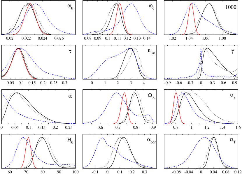
We assign flat (i.e., uniform over some range; see Appendix) prior probabilities to our 10 primary parameters, using the amplitude parametrization. Since some parameters are not tightly constrained by the data, the posterior likelihoods depend somewhat on the prior probability densities. To show the effect of the priors, and to compare to [4], we used the Jacobian of the parameter transformation (see Appendix) to convert the 1-d marginalized likelihoods obtained from our chains to correspond to flat priors for the index parametrization (dotted lines in Fig. 1).

4 Results

Figure 1: Marginalized likelihood functions for selected primary and derived parameters. The solid black curves are our new results using WMAP 3-year data and Boomerang data from the 2003 flight (+ ACBAR & SDSS). The dotted black curves show the effect of assigning flat priors in the index parametrization instead of the amplitude parametrization. The red/gray curves are for an adiabatic model using the same data. The dashed blue curves are from our previous study [4] using data available in 2004. Note that also in the adiabatic model WMAP3 data favors a larger $H_{0}$ than WMAP1 (not shown)—allowing isocurvature modes favors larger $H_{0}$ regardless of which WMAP data set is used, although the effect is much stronger with WMAP3.

Table 1: The best-fit models. A: The full model with a correlated isocurvature mode. B: The adiabatic model.

• 	$\omega_{b}$	$\omega_{c}$	$100\theta$	$\tau$	$n_{\rm{ad1}}$	$n_{\rm{ad2}}$	$n_{\rm{iso}}$	$\alpha$	$\gamma$
  A	0.0223	0.1066	1.062	0.0914	0.975	0.919	3.54	0.0539	0.180
  B	0.0224	0.1124	1.042	0.0856	0.960

• 	$\Omega_{\Lambda}$	$H_{0}$	$\sigma_{8}$	$\alpha_{\rm{cor}}$	$\alpha_{T}$
  A	0.800	80.3	1.11	0.096	0.0356
  B	0.734	71.2	0.80

We show 1-d marginalized likelihoods for selected primary and derived parameters in Fig. 1. Instead of the amplitudes at $k_{1}$ and $k_{2}$ we show the derived parameters: spectral index $n_{\rm{iso}}$ and the amplitude parameters $\alpha$ and $\gamma$ at the intermediate scale $k_{0}=0.01\mbox{Mpc}^{-1}$. The mappings between these are presented in the Appendix.

The data lead to likelihood peaks at clearly nonzero values for $\alpha$ (the ratio of the primordial entropy perturbation power to the total perturbation power at $k_{0}$) and favor a positive $\gamma$. (This significantly reduces the pivot-scale dependence of the likelihoods discussed in [4].) If the subdominant entropy perturbation is correlated with the dominant curvature perturbation it has a much stronger effect on the observables. To account for this we also show $\alpha_{\rm{cor}}\equiv\mathrm{sign}(\gamma)\sqrt{\alpha(1-\alpha)|\gamma|}$, which gives the relative “weight” of the correlation spectrum $C_{\ell}^{\mathrm{cor}}$ in $C_{\ell}$, see Equation (3). We find $\alpha=0.082\pm 0.046$ (mean $\pm$ stdev), with $\alpha<0.169$ at 95% C.L. and $\alpha_{\rm{cor}}=0.139\pm 0.055$, with $0.044<\alpha_{\rm{cor}}<0.252$ at 95% C.L. The correlation between the isocurvature and adiabatic modes is positive, $\gamma>0.051$ at 95% C.L.

These values are obtained from the likelihood functions corresponding to the amplitude parametrization with flat priors for the primary parameters. As can be seen from Fig. 1 the exact confidence levels depend on the assumed priors, but the conclusions are not changed at a qualitative level. We discuss the priors more in the Appendix.

Since the definitions of the primary amplitude parameters (e.g. $\alpha$) depend on the choice of pivot scale, we also define

$$\alpha_{T}\equiv\frac{\sum(2\ell+1)(C_{\ell}^{\mathrm{iso}}+C_{\ell}^{\mathrm{cor}})}{\sum(2\ell+1)C_{\ell}}\,,$$ (6)

the total nonadiabatic contribution to the CMB temperature variance,

$$\Bigg{\langle}\left(\frac{\delta T}{T}\right)^{2}\Bigg{\rangle}=\sum_{\ell}\frac{2\ell+1}{4\pi}C_{\ell}\,.$$ (7)

We find $\alpha_{T}=0.043\pm 0.015$, and the whole 95% C.L. range $0.017<\alpha_{T}<0.073$ is positive. Thus the CMB data clearly favor a nonadiabatic contribution.

Our best-fit model and also the best-fit adiabatic model are given in Table I. They are compared in Fig. 2. The WMAP 3-year data prefer a slightly narrower 2nd peak than the adiabatic model can produce. This holds for the third peak also, but now the peak position and width are determined by the Boomerang data.

Figure 2: The CMB temperature angular power spectrum for our best-fit model (black) compared to the best-fit adiabatic model (red/gray). The dashed blue curve shows the nonadiabatic contribution. The inset shows the 2nd and 3rd peaks.

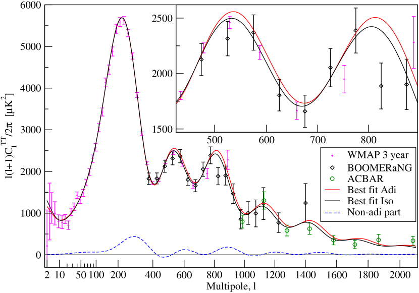
This feature in the data can be accounted for by a correlated isocurvature component. It can narrow down the 2nd peak without affecting the 1st peak position, which is accurately determined by the data. Increasing $\theta$ shifts the whole peak structure to the left, making the peaks narrower. Adding a positively correlated isocurvature component returns the 1st peak to its place.

Compared to the adiabatic model, adding 4 parameters improved the fit by $\Delta\chi^{2}=9.7$. This comes mainly from the fit to the WMAP and Boomerang temperature (TT) $C_{\ell}$; for the WMAP part from the 2nd peak. The data on the TE and EE $C_{\ell}$ are too inaccurate for a few per cent isocurvature contribution to play any role. Therefore the contribution to $\chi^{2}$ from these cross-correlation data is the same for the adabatic and our model. The fit to the SDSS data has improved slightly, whereas that to the ACBAR data is indifferent. In Table 2 we give quantitative numbers for the contributions of different data sets to the best-fit models. The best-fit model and its $\chi^{2}$ with the data are of course not affected by the issue of priors, which affects only the likelihoods. For the first time in the history of CMB temperature anisotropy observations, adding the CDM (or baryon) isocurvature degree of freedom improves the fit to the data, and the likelihoods of isocurvature parameters peak at non-zero values, as seen in Tables 1 & 2 and Fig. 1.

Table 2: The $\chi^{2}$ of the fit of the best-fit models to the data, and the contributions from the four different data sets. A: The full model with a correlated isocurvature mode. B: The adiabatic model.

• data set	$\chi^{2}$ (A)	$\chi^{2}$ (B)	$\Delta\chi^{2}$
  WMAP	3535.20	3539.14	3.94
  Boomerang	31.12	35.04	3.92
  ACBAR	10.10	9.92	$-0.18$
  SDSS LRG	22.64	24.66	2.02
  total	3599.06	3608.78	9.72

The other major effect is that the correlated isocurvature model favors a smaller CDM density $\omega_{c}$ (also $\omega_{b}$ is down, but not as much). This is due to the correlation component $C_{\ell}^{\mathrm{cor}}$, which raises the first and third peaks with respect to the second one. See Fig. 2. Lower $\omega_{m}$ and $\omega_{b}$ compensate this by raising the second peak.

For fixed $\omega_{c}$ and $\omega_{b}$, increasing $\theta$ leads to a larger $\Omega_{\Lambda}$ and a larger Hubble constant $H_{0}$. For fixed $\theta$ and $\omega_{b}$, a lower $\omega_{c}$ requires an even larger $\Omega_{\Lambda}$ and $H_{0}$. Therefore these models have a larger $H_{0}$ and a smaller matter density parameter $\Omega_{m}=1-\Omega_{\Lambda}$, than the adiabatic model.

5 Other cosmological data

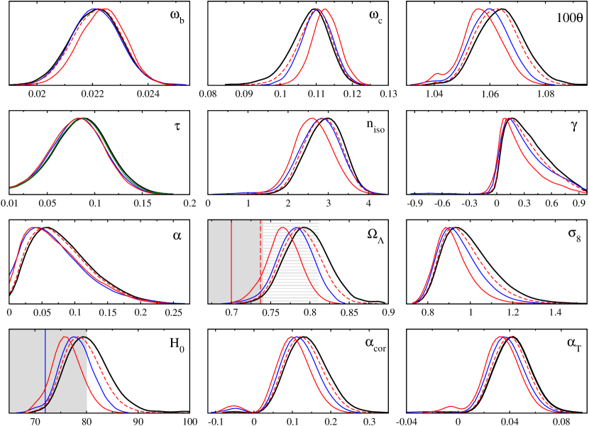
The large $H_{0}=80\pm 4\mathrm{km/s/Mpc}$ and small $\Omega_{m}=0.204\pm 0.028$ of our nonadiabatic model is in some tension with other cosmological data, like the Hubble Space Telescope (HST) value for the Hubble constant, $H_{0}=72\pm 8\mathrm{km/s/Mpc}$ [31] and the estimates of $\Omega_{m}$ from Supernova Ia data ($\Omega_{m}=0.29^{+0.05}_{-0.03}$ from [32], or $\Omega_{m}=0.263\pm 0.042\pm 0.032$ from [33]). To assess the effect of an $\Omega_{m}$ constraint, we postprocessed our likelihoods by weighting (importance sampling [25]) our MCMC chains with corresponding Gaussian distributions for $\Omega_{m}$. We also ran new MCMC chains with a Gaussian $H_{0}=72\pm 8\mathrm{km/s/Mpc}$ [31] prior. The results are shown in Fig. 3. The effect of the weaker $\Omega_{m}=0.263\pm 0.074$ prior is minor and does not eliminate the favoring of nonzero $\alpha$ and positive $\alpha_{T}$. The same is true for the $H_{0}$ prior, although now the 95% C.L. range $-0.005<\alpha_{T}<0.065$ includes $\alpha_{T}=0$. An $\Omega_{m}=0.30\pm 0.04$ prior has a larger effect, but the 1-d likelihood of $\alpha$ appears still to peak at a nonzero value.

Figure 3: Marginalized likelihood functions for selected primary and derived parameters after including additional priors coming from other cosmological data. The solid black curves are the same as in Fig.1. The solid blue curves show the effect of adding the HST $H_{0}$ prior. The solid red curves show the effect of the stronger $\Omega_{m}=0.29^{+0.05}_{-0.03}$ prior and the dashed red curves are for the weaker $\Omega_{m}=0.263\pm 0.074$ prior. The central values and 1-$\sigma$ ranges of these Gaussian priors are indicated by vertical lines and gray areas in the $\Omega_{\Lambda}$ and $H_{0}$ panels.

As noted in [4], $n_{\rm{iso}}\simeq 3$ (when $n_{\rm{ad}}\simeq 1$) means that the relative isocurvature contribution to $C_{\ell}$ is about the same on all scales, but in the LSS power spectrum the isocurvature and correlation components overtake the adiabatic ones at small scales. Thus there is more (matter) power at small scales, with a larger rms mass fluctuation on 8 $h^{-1}$Mpc scale $\sigma_{8}$. While the adiabatic model favors $\sigma_{8}\approx 0.8$, our model favors $\sigma_{8}\approx 1$. Assuming the power law is a good approximation for the primordial spectra also at smaller scales, Lyman-$\alpha$ data can constrain $n_{\rm{iso}}$ [34]. Creating new MCMC chains with Lyman-$\alpha$ data included like in [34] we checked that the peak in the likelihood of $n_{\rm{iso}}$ shifted to $2.1$, and $\alpha$ to zero. The other likelihoods became more like in the adiabatic case. The peak in $\alpha_{T}$ remained clearly positive, but the 68% C.L. region, $\alpha_{T}=0.022^{+0.017}_{-0.025}$, now included $\alpha_{T}=0$. Thus the large small-scale power implied by a relatively large constant $n_{\rm{iso}}$ means that inclusion of small-scale data significantly weakens the preference for a nonadiabatic contribution. One possible interpretation is that $n_{\rm{iso}}$ is not a constant, but becomes smaller for the large $k$ probed by Lyman-$\alpha$ data.

6 Discussion

The acoustic peak structure in the latest CMB data favors a few per cent nonadiabatic contribution. Our best fit to the CMB + LSS data has a significant contribution from a positively correlated isocurvature mode, so that the isocurvature fraction, i.e., the ratio of primordial entropy perturbation power to total perturbation power at the scale of $k=0.01\mathrm{\leavevmode\nobreak\ Mpc}^{-1}$, is 5% and the nonadiabatic contribution to CMB temperature variance is 4%. With the addition of four model parameters, the fit to the data improved by $\Delta\chi^{2}=9.7$, which can already be considered interesting.

We note that the nonadiabatic models that give the best fits to the CMB data, have some problems with other cosmological data. These problems may be remedied if one considers non-flat models. A preliminary look at these models seems to indicate that the best-fit non-flat models are closed models with a total energy density a few per cent over the critical density, a Hubble constant close to the HST value, $\Omega_{m}$ and $\Omega_{\Lambda}$ in agreement with the SNIa data, the isocurvature spectral index $n_{\rm{iso}}$ closer to 2 than 3, and an even larger nonadiabatic contribution than in the case of flat nonadiabatic models.

While interesting, the preference for nonadiabatic primordial perturbations discovered in this study should not be taken as conclusive evidence for a primordial isocurvature mode. It is not yet at a very high confidence level, so the possibility remains that it is just a statistical fluke. Other possible explanations are an unaccounted for systematic effect in the WMAP and Boomerang data, or some other nonstandard cosmological feature whose effect on the CMB is in a similar direction. It remains for the future more precise CMB measurements to resolve this. If the presence of a primordial isocurvature mode were confirmed, it would automatically rule out single-field inflation, since generating a primordial entropy perturbation requires more than one degree of freedom.

Appendix A Priors and parametrizations

When some parameters of a model are not sufficiently tightly constrained by the data, the posterior likelihood functions become sensitive to the assumed prior probability densities for the parameters. Even when one assumes flat, i.e., uniform, priors for the primary parameters of the model, the question remains, which parameters are taken to be the primary parameters, since the priors for the quantities derived from the primary parameters (derived parameters) will not be flat. To avoid problems related to spectral indices becoming unconstrained when the corresponding amplitude parameters have small values, we introduced in this study a parametrization in terms of amplitudes at two different scales, instead of using spectral indices as primary parameters.

Mapping from the amplitude parametrization to the spectral index parametrization is easy to find by employing definitions (2), (4), and (5). The spectral indices can be written in terms of the parameters of amplitude parametrization as

$$n_{\rm{ad1}}-1=\frac{\ln\left[\mathcal{P}_{\mathcal{R}1}(k_{2})/\mathcal{P}_{\mathcal{R}1}(k_{1})\right]}{\ln(k_{2}/k_{1})}\,,$$ (8)

$$n_{\rm{ad2}}-1=\frac{\ln\left[\mathcal{P}_{\mathcal{R}2}(k_{2})/\mathcal{P}_{\mathcal{R}2}(k_{1})\right]}{\ln(k_{2}/k_{1})}\,,$$ (9)

$$n_{\rm{iso}}-1=\frac{\ln\left[\mathcal{P}_{\mathcal{S}}(k_{2})/\mathcal{P}_{\mathcal{S}}(k_{1})\right]}{\ln(k_{2}/k_{1})}\,,$$ (10)

where the first (uncorrelated) adiabatic, the second (correlated) adiabatic and the isocurvature power spectra at scales $k_{i}$ ($i=1,2$) are given by

$$\mathcal{P}_{\mathcal{R}1}(k_{i})=A_{i}^{2}(1-\alpha_{i})(1-|\gamma_{i}|)\,,$$ (11)

$$\mathcal{P}_{\mathcal{R}2}(k_{i})=A_{i}^{2}(1-\alpha_{i})|\gamma_{i}|\,,$$ (12)

$$\mathcal{P}_{\mathcal{S}}(k_{i})=A_{i}^{2}\alpha_{i}\,,$$ (13)

respectively. Then the amplitudes $A$, $\alpha$, and $\gamma$ at $k_{0}=0.01\;$Mpc^-1 are obtained from the amplitude-parametrization amplitudes $A_{1}$, $\alpha_{1}$, and $\gamma_{1}$ defined at $k_{1}=0.002\;$Mpc^-1 by [4]

$$A^{2}=A_{1}^{2}\Big{[}(1-\alpha_{1})(1-|\gamma_{1}|)\tilde{k}^{n_{\rm{ad1}}-1}+(1-\alpha_{1})|\gamma_{1}|\tilde{k}^{n_{\rm{ad2}}-1}+\alpha_{1}\tilde{k}^{n_{\rm{iso}}-1}\Big{]}\,,$$ (14)

$$\alpha=\frac{\alpha_{1}\tilde{k}^{n_{\rm{iso}}-1}}{(1-\alpha_{1})(1-|\gamma_{1}|)\tilde{k}^{n_{\rm{ad1}}-1}+(1-\alpha_{1})|\gamma_{1}|\tilde{k}^{n_{\rm{ad2}}-1}+\alpha_{1}\tilde{k}^{n_{\rm{iso}}-1}}\,,$$ (15)

$$\gamma=\frac{\gamma_{1}\tilde{k}^{n_{\rm{ad2}}-1}}{(1-|\gamma_{1}|)\tilde{k}^{n_{\rm{ad1}}-1}+|\gamma_{1}|\tilde{k}^{n_{\rm{ad2}}-1}}\,,$$ (16)

where $\tilde{k}=k_{0}/k_{1}$, and the spectral indices are obtained from Eqs. (8)–(10).

If we take as a starting point the spectral index parametrization, then the mapping from it to the amplitude parametrization is simply

$$A_{i}^{2}=A^{2}\Big{[}(1-\alpha)(1-|\gamma|)\tilde{k}^{n_{\rm{ad1}}-1}+(1-\alpha)|\gamma|\tilde{k}^{n_{\rm{ad2}}-1}+\alpha\tilde{k}^{n_{\rm{iso}}-1}\Big{]}\,,$$ (17)

$$\alpha_{i}=\frac{\alpha\tilde{k}^{n_{\rm{iso}}-1}}{(1-\alpha)(1-|\gamma|)\tilde{k}^{n_{\rm{ad1}}-1}+(1-\alpha)|\gamma|\tilde{k}^{n_{\rm{ad2}}-1}+\alpha\tilde{k}^{n_{\rm{iso}}-1}}\,,$$ (18)

$$\gamma_{i}=\frac{\gamma\tilde{k}^{n_{\rm{ad2}}-1}}{(1-|\gamma|)\tilde{k}^{n_{\rm{ad1}}-1}+|\gamma|\tilde{k}^{n_{\rm{ad2}}-1}}\,,$$ (19)

where $\tilde{k}=k_{i}/k_{0}$ and $i=1,2$.

Since we assume that all the component spectra can be described by power laws, $\gamma_{1}$ and $\gamma_{2}$ must have the same sign. Hence, they are not completely independent. To obtain independent primary parameters, we draw $\gamma_{1}$ from the range $[-1,1]$, but $\gamma_{2}$ only from the range $[0,1]$, and let $\gamma_{1}$ determine the sign of the correlation. This has no effect on formulas (8) – (18), but to maintain consistency we need to modify equation (19). Instead of $\gamma$ we should have in the nominator $|\gamma|$, if $i=2$.

Employing mappings (8) – (10) and (14) – (16) we obtain the posterior likelihoods of $n_{\rm{ad1}}$, $n_{\rm{ad2}}$, $n_{\rm{iso}}$, $A$, $\alpha$, $\gamma$ for a MCMC run in the amplitude parametrization (corresponding to flat priors for $A_{1}$, $\alpha_{1}$, $\gamma_{1}$, $A_{2}$, $\alpha_{2}$, and $\gamma_{2}$). Likewise, if a MCMC run was made in spectral index parametrization, we could use mappings (17) – (19) to obtain the posterior likelihoods of $A_{1}$, $\alpha_{1}$, $\gamma_{1}$, $A_{2}$, $\alpha_{2}$, $\gamma_{2}$ (and other parameters) corresponding to flat prior probabilities for the primary parameters of the index parametrization.

However, if we want to convert the results obtained in the amplitude parametrization to flat priors for the spectral indices, then the mapping (8) – (10) and (14) – (16) is not enough. We have to correct for the prior too. This can be done by weighting the multiplicities in the MCMC chains (i.e. weighting the posterior likelihood) by the Jacobian of the transformation (8) – (10) and (14) – (16). If the MCMC run was made using primary parameters $\{\Theta_{i}\}$ (and flat priors for them), but we want to show the results with flat priors for $\{\tilde{\Theta}_{i}\}$, the multiplicities must be multiplied by

$$J=\left|\det\left(\frac{\partial\Theta_{i}}{\partial\tilde{\Theta}_{j}}\right)\right|\,.$$ (20)

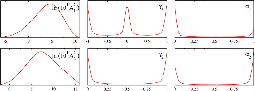
In Figs. 4 and 5 we show what the priors of one parametrization become when the priors of the other parametrization are taken to be flat.

In the amplitude parametrization the range of parameters (which is also a crucial part of the prior) is throughout our study

$$\omega_{b}\in[0.005,0.1],\quad\omega_{c}\in[0.01,0.99],\quad 100\theta\in[0.3,10.0],\quad\tau\in[0.01,0.3]$$

$$\ln(10^{10}A_{1}^{2})\in[1,7],\quad\alpha_{1}\in[0,1],\quad\gamma_{1}\in[-1,1]$$

$$\ln(10^{10}A_{2}^{2})\in[1,7],\quad\alpha_{2}\in[0,1],\quad\gamma_{2}\in[0,1]\,.$$

In the spectral index parametrization the range of background parameters is the same as above, and the perturbation parameters have a uniform prior probability over the ranges

$$n_{\rm{ad1}}\in[-3,4],\quad n_{\rm{ad2}}\in[-3,4],\quad n_{\rm{iso}}\in[-3,12],$$

$$\ln(10^{10}A^{2})\in[1,7],\quad\alpha\in[0,1],\quad\gamma\in[-1,1]\,.$$

These are used only for producing Fig. 5, since all our analysis presented in this paper is based on MCMC runs in the amplitude parametrization. However, we have checked against a MCMC run using the index parametrization, that its results agree with the dotted black curves in Fig. 1 (which were obtained from the MCMC run using amplitude parametrization by correcting for the prior with the Jacobian (20)). For Fig. 5 we chose the above ranges of spectral indices to match this check run and our previous study [4]. As indices are not symmetric around the scale invariance ($n=1$), we can see mild asymmetries in Fig. 5.

Figure 4: The red curves show the priors for the parameters of the index parametrization, when flat priors are assumed for the parameters of the amplitude parametrization. The black curves are the posterior likelihoods we have obtained (the same as the solid black curves in Fig. 1).

Figure 5: The priors for the parameters of the amplitude parametrization, when flat priors are assumed for the parameters of the index parametrization.

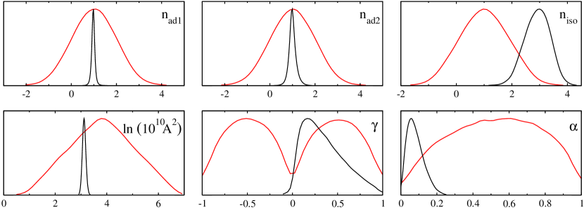
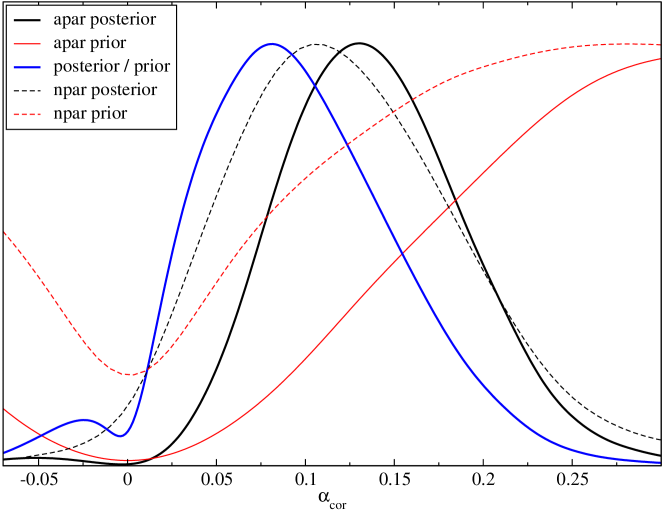
The parameters $\alpha_{\rm{cor}}$ and $\alpha_{T}$ are derived parameters and therefore their prior distributions are not flat in either parametrization. We demonstrate the situation with $\alpha_{\rm{cor}}$ in Fig. 6. We see that $\alpha_{\rm{cor}}$ as well as the parameters $n_{\rm{iso}}$, $\gamma$, and $\alpha$ (see Fig. 4) are not well enough determined by the data to make their likelihood functions insensitive to the choice of priors. The solid blue curve in Fig. 6 is the ratio of the posterior and prior likelihoods for $\alpha_{\rm{cor}}$, and illustrates what the likelihood of $\alpha_{\rm{cor}}$ could be, if $\alpha_{\rm{cor}}$ had a flat prior probability density. The actual likelihood of course depends also on the other priors.

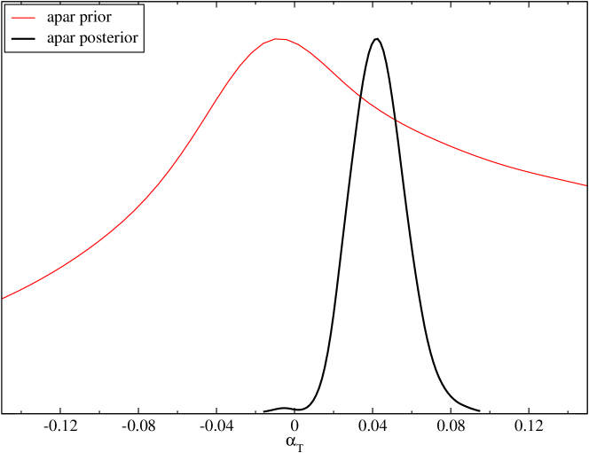
In Fig. 7 we show the prior and posterior distributions of $\alpha_{T}$ in the amplitude parametrization. We see that the prior is relatively flat in the region where the posterior mostly lies. Consequently, unlike for $\alpha_{\rm{cor}}$ the ratio of posterior and prior likelihoods (posterior/prior) for $\alpha_{T}$ is almost indistinguishable from the posterior. Thus the situation with $\alpha_{T}$ is better in this respect than the case of $\alpha_{\rm{cor}}$, and the conclusions about $\alpha_{T}$ are more robust.

Figure 6: Prior and posterior likelihoods for the derived parameter $\alpha_{\rm{cor}}$. The solid red curve is the prior in the amplitude parametrization and the dashed red curve is the same in the index parametrization. The solid and dashed black curves are the corresponding posterior likelihoods. These are the same as the solid and dotted black curves in the $\alpha_{\rm{cor}}$ panel of Fig. 1. The solid blue curve is the ratio of the posterior and prior likelihoods in the amplitude parametrization.

Figure 7: Prior thin red and posterior thick black likelihoods for the derived parameter $\alpha_{T}$. Both likelihoods are for the amplitude parametrization. Posterior/prior would be almost indistinguishable from the posterior.

References

- [1] M. Bucher, K. Moodley, and N. Turok, The general primordial cosmic perturbation, Phys. Rev. D62 (2000) 083508, [astro-ph/9904231].
- [2] K. Enqvist, H. Kurki-Suonio, and J. Valiviita, Open and closed cdm isocurvature models contrasted with the cmb data, Phys. Rev. D65 (2002) 043002, [astro-ph/0108422].
- [3] K. Enqvist, H. Kurki-Suonio, and J. Valiviita, Limits on isocurvature fluctuations from Boomerang and MAXIMA, Phys. Rev. D62 (2000) 103003, [astro-ph/0006429].
- [4] H. Kurki-Suonio, V. Muhonen, and J. Valiviita, Correlated primordial perturbations in light of cmb and lss data, Phys. Rev. D71 (2005) 063005, [astro-ph/0412439].
- [5] D. Langlois, Correlated adiabatic and isocurvature perturbations from double inflation, Phys. Rev. D59 (1999) 123512, [astro-ph/9906080].
- [6] C. L. Bennett et al., First year wilkinson microwave anisotropy probe (wmap) observations: Preliminary maps and basic results, Astrophys. J. Suppl. 148 (2003) 1, [astro-ph/0302207].
- [7] J. Valiviita and V. Muhonen, Correlated adiabatic and isocurvature cmb fluctuations in the wake of wmap, Phys. Rev. Lett. 91 (2003) 131302, [astro-ph/0304175].
- [8] M. Beltran, J. Garcia-Bellido, J. Lesgourgues, A. R. Liddle, and A. Slosar, Bayesian model selection and isocurvature perturbations, Phys. Rev. D71 (2005) 063532, [astro-ph/0501477].
- [9] H. V. Peiris et al., First year wilkinson microwave anisotropy probe (wmap) observations: Implications for inflation, Astrophys. J. Suppl. 148 (2003) 213, [astro-ph/0302225].
- [10] P. Crotty, J. Garcia-Bellido, J. Lesgourgues, and A. Riazuelo, Bounds on isocurvature perturbations from cmb and lss data, Phys. Rev. Lett. 91 (2003) 171301, [astro-ph/0306286].
- [11] D. Parkinson, S. Tsujikawa, B. A. Bassett, and L. Amendola, Testing for double inflation with wmap, Phys. Rev. D71 (2005) 063524, [astro-ph/0409071].
- [12] K. Moodley, M. Bucher, J. Dunkley, P. G. Ferreira, and C. Skordis, Constraints on isocurvature models from the wmap first-year data, Phys. Rev. D70 (2004) 103520, [astro-ph/0407304].
- [13] F. Ferrer, S. Rasanen, and J. Valiviita, Correlated isocurvature perturbations from mixed inflaton- curvaton decay, JCAP 0410 (2004) 010, [astro-ph/0407300].
- [14] M. Beltran, J. Garcia-Bellido, J. Lesgourgues, and A. Riazuelo, Bounds on cdm and neutrino isocurvature perturbations from cmb and lss data, Phys. Rev. D70 (2004) 103530, [astro-ph/0409326].
- [15] C. J. MacTavish et al., Cosmological parameters from the 2003 flight of boomerang, Astrophys. J. 647 (2006) 799, [astro-ph/0507503].
- [16] D. N. Spergel et al., Wilkinson microwave anisotropy probe (wmap) three year results: Implications for cosmology, astro-ph/0603449.
- [17] R. Bean, J. Dunkley, and E. Pierpaoli, Constraining isocurvature initial conditions with wmap 3- year data, Phys. Rev. D74 (2006) 063503, [astro-ph/0606685].
- [18] A. Lewis, Observational constraints and cosmological parameters, astro-ph/0603753.
- [19] R. Trotta, The isocurvature fraction after wmap 3-year data, astro-ph/0608116.
- [20] W. C. Jones et al., A measurement of the angular power spectrum of the cmb temperature anisotropy from the 2003 flight of boomerang, Astrophys. J. 647 (2006) 823, [astro-ph/0507494].
- [21] M. Tegmark et al., Cosmological constraints from the sdss luminous red galaxies, astro-ph/0608632.
- [22] C. Gordon, D. Wands, B. A. Bassett, and R. Maartens, Adiabatic and entropy perturbations from inflation, Phys. Rev. D63 (2001) 023506, [astro-ph/0009131].
- [23] L. Amendola, C. Gordon, D. Wands, and M. Sasaki, Correlated perturbations from inflation and the cosmic microwave background, Phys. Rev. Lett. 88 (2002) 211302, [astro-ph/0107089].
- [24] C. T. Byrnes and D. Wands, Curvature and isocurvature perturbations from two-field inflation in a slow-roll expansion, Phys. Rev. D74 (2006) 043529, [astro-ph/0605679].
- [25] A. Lewis and S. Bridle, Cosmological parameters from cmb and other data: a monte- carlo approach, Phys. Rev. D66 (2002) 103511, [astro-ph/0205436].
- [26] A. Gelman and D. Rubin, Inference from iterative simulation using multiple sequences, Statistical Science 7 (1992) 457.
- [27] L. Page et al., Three year wilkinson microwave anisotropy probe (wmap) observations: Polarization analysis, astro-ph/0603450.
- [28] G. Hinshaw et al., Three-year wilkinson microwave anisotropy probe (wmap) observations: Temperature analysis, astro-ph/0603451.
- [29] ACBAR Collaboration, C.-l. Kuo et al., High resolution observations of the cmb power spectrum with acbar, Astrophys. J. 600 (2004) 32–51, [astro-ph/0212289].
- [30] SDSS Collaboration, M. Tegmark et al., The 3d power spectrum of galaxies from the sdss, Astrophys. J. 606 (2004) 702–740, [astro-ph/0310725].
- [31] W. L. Freedman et al., Final results from the hubble space telescope key project to measure the hubble constant, Astrophys. J. 553 (2001) 47–72, [astro-ph/0012376].
- [32] Supernova Search Team Collaboration, A. G. Riess et al., Type ia supernova discoveries at from the hubble space telescope: Evidence for past deceleration and constraints on dark energy evolution, Astrophys. J. 607 (2004) 665–687, [astro-ph/0402512].
- [33] P. Astier et al., The supernova legacy survey: Measurement of , and w from the first year data set, Astron. Astrophys. 447 (2006) 31–48, [astro-ph/0510447].
- [34] M. Beltran, J. Garcia-Bellido, J. Lesgourgues, and M. Viel, Squeezing the window on isocurvature modes with the lyman- alpha forest, Phys. Rev. D72 (2005) 103515, [astro-ph/0509209].