Multi-scale morphology of the galaxy distribution

Abstract

Many statistical methods have been proposed in the last years for analyzing the spatial distribution of galaxies. Very few of them, however, can handle properly the border effects of complex observational sample volumes. In this paper, we first show how to calculate the Minkowski Functionals (MF) taking into account these border effects. Then we present a multiscale extension of the MF which gives us more information about how the galaxies are spatially distributed. A range of examples using Gaussian random fields illustrate the results. Finally we have applied the Multiscale Minkowski Functionals (MMF) to the 2dF Galaxy Redshift Survey data. The MMF clearly indicates an evolution of morphology with scale. We also compare the 2dF real catalog with mock catalogs and found that $\Lambda$CDM simulations roughly fit the data, except at the finest scale.

1 Introduction

One of the main tenets of the present inflationary paradigm is the assumption of Gaussianity for the primordial density perturbations. This postulate forms the basis of present theories of formation and evolution of large-scale structure in the universe, and of its subsequent analysis. But it remains a hypothesis that needs to be checked.

The most straightforward way to do that would be to follow the definition of Gaussian random fields (see, e.g, Adler (1981)) – their one-point probability distribution and all many-point joint probability distributions of field amplitudes have to be Gaussian. This is clearly a too formidable task. Another way is to check the relationships between the correlation functions and power spectra of different orders, which are well-defined for Gaussian random fields. This approach is frequently used (see, e.g., a review in Martínez & Saar (2002)). A third method is to study the morphology of the cosmological (density) fields. One approach to the morphological description relies on the so-called Minkowski functionals and is complementary to the moment-based methods because these functionals depend on moments of all orders. This procedure has been usually referred to as topological analysis. It has a quite long history already, starting with the seminal paper by Gott et al. (1986), that deals with the genus, a quantity closely related to one of the four Minkowski functionals. The approach in the present paper lies within this latter framework; we describe it in detail in Sec. 2.

There are two different possibilities to develop a morphological analysis of galaxy catalogues based on Minkowski functionals. First, we can dress all points (galaxies) with spheres of a given radius, and study the morphology of the surface that is generated by the convex union of these spheres, as a function of the radius, which acts here as the diagnostic parameter. An appropriate theoretical model to compare with in this case is a Poisson point process. On the other hand, if we wish to study the morphology of the underlying realization of a random field, we have to restore the (density) field first, to choose an isodensity surface corresponding to a given density threshold and to calculate its morphological descriptors. In this approach the density threshold (or a related quantity) acts as the diagnostic parameter. The theoretical reference model is that of a Gaussian random field, and the crucial point here is to properly choose a restoration method that provides a smoothed underlying density field that should be fairly sampled by the observed discrete point distribution.

Starting from the original paper on topology by Gott et al. (1986), this task has been typically done by smoothing the point distribution with a Gaussian kernel. The choice of the optimal width of this kernel has been widely discussed; it is usually taken close to the correlation length of the point distribution. However, Gaussian smoothing is not the best choice for morphological studies. As we have shown recently (Martínez et al., 2005), it tends to introduce additional Gaussian features even for manifestly non-Gaussian density distributions. Minkowski functionals are very sensitive to small density variations, and the wings of Gaussian kernels could be wide enough to generate a small-amplitude Gaussian ripple that is added to the true density distribution. Such effect could be alleviated by using compact adaptive smoothing kernels, as we show below.

It is well known that large-scale cosmological fields have a multi-scale structure. A good example is the density field; it includes components that vary on widely different sales. The amplitudes of these components can be characterized by the power spectrum; the present determinations encompass the frequency interval 0.01–0.8 $h$/Mpc, which corresponds to the scale range from 8 to over 600 Mpc/$h$. Fig. 1 shows the power spectrum for the 2dF galaxy redshift survey (2dFGRS).

As cosmological densities have many scales and widely varying amplitudes, density restoration should be adaptive. Different methods exist to adaptively smooth point distributions to estimate from them the underlying density field. Schaap & van de Weygaert (2000) have introduced the Delaunay Tessellation Field Estimator (DTFS) which adapts itself to the point configuration even when anisotropies are present. The method starts by considering the Delaunay tessellation of the point process, then we can estimate the density at those points using the contiguous Voronoi cells, and finally, we should interpolate to obtain the density in the whole volume. Intricate point patterns have been successfully smoothed using this method and applications to particle hydrodynamics provide good performance (Pelupessy et al., 2003). Ascasibar & Binney (2005) have recently introduced a novel technique based on a different partition of the embedding space. These authors use multidimensional binary trees to make the partition and latter apply adaptive kernels within the resulting cells. Finally, it is well known that wavelets provide a localized (compact-kernel) adaptive restoration method (Starck & Murtagh, 2002). We have applied, in a previous paper (Martínez et al., 2005), a wavelet based denoising technique to the 2dFGRS. As a result we found that the morphology of the galaxy density distribution in the survey volume does not follow a Gaussian pattern, in contrast to the usual results in which deviations of Gaussianity are not clearly detected (see, e.g., Hoyle et al. (2002) for the 2dFGRS and Park et al. (2005) for the Sloan Digital Sky Survey (SDSS)).

Figure 1: The matter density power spectrum for the 2dF GRS. Data courtesy of W. Percival and the 2dF GRS team.

By the way, adaptive density restoration methods are probably the best for calculating partial Minkowski functionals, to describe the morphology of single large-scale density enhancements (superclusters; see, e.g., Shandarin et al. (2004)). Partial functionals can be used to characterize the inner structure (clumpiness) and shapes (via shapefinders (Sahni et al., 1998)) of superclusters. As Minkowski functionals are additive, partial functionals can be, in principle, combined to obtain global Miknkowski functionals for the whole catalogue volume. But if we want to check for non-Gaussianity, direct calculation of global Minkowski functionals is more simple and straightforward. When combining partial functionals, estimating the mean densities and volume distributions for the full sample is a difficult problem.

Now, although a single adaptively found density distribution represents the cosmological density field better, it could not be the best tool for comparing theories with observations. Theories of evolution of structure predict that Gaussianity of the original density distribution is distorted during evolution, and this distortion is scale-dependent. According to the present paradigm, evolution of structure should proceed with different pace at different scales. At smaller scales signatures of gravitational dynamics should be seen, and traces of initial conditions could be discovered at larger scales. In a single density field, containing contributions from all scales, these effects are mixed. Thus, a natural way to study cosmological density fields is the multi-scale approach, scale by scale. This has been done in the past by using a series of kernels of different width (Park et al., 2005), but this method retains considerable low-frequency overlap. A better way is to decompose the density field into different frequency (scale) subbands, and to study each subband separately.

The simplest idea of separation of scales by using different Fourier modes does not work well, at least for morphological studies (studies of shapes and texture). Describing texture requires knowledge of positions, but Fourier modes do not have positions, their position is the whole sample space. A similar weakness, to a smaller extent, is shared by discrete orthogonal wavelet expansions – their localisation properties are better, but vary with scale, and large-scale modes remain badly localised.

This leads to the conclusion that the natural candidates for scale separation are shift-invariant wavelet systems, where wavelet amplitudes of all scales are calculated for each point of the coordinate grid. These wavelet decompositions are redundant – each subband has the same data volume as the original data.

For such a scheme, direct calculation of low-frequency subbands would require convolution with wide wavelet profiles, that could be numerically expensive. A way out is the à trous (with holes) trick, where convolution kernels for the next dyadic scale are obtained by inserting zeros between the elements of the original kernel. In this way, the total number of non-zero elements is the same for all kernels, and all wavelet transforms are equally fast.

Now, as usual with wavelets, there is considerable freedom in choosing the wavelet kernel. A particularly useful choise is the wavelet based on a $B_{3}$ spline scaling function (see Appendix A). In this case, the original data can be reconstructed as a simnple sum of subbands, without extra weights, so the subband decomposition is the most natural.

In the present paper we combine the à trous representation of density fields with a grid-based algorithm to calculate the Minkowski functionals (MF for short), and apply it to the 2dFGRS data.

Section 2 describes how to compute the MF for complex data volumes and how to extend such an approach in a multiscale framework using the wavelet transform. Section 3 describes our observational data while section 4 evaluates the multiscale MF on Gaussian random field realizations for which the analytical results are known. Section 5 presents our results for the 2dFGRS data. These results are compared with the multiscale MF calculated for 22 mock surveys and about 100 Monte-Carlo simulations of Gaussian random fields. We list the conclusions in section 6.

2 Morphological analysis

2.1 Definition

An elegant description of morphological characteristics of density fields is given by Minkowski functionals (Mecke et al., 1994). These functionals provide a complete family of morphological measures. In fact all additive, motion invariant and conditionally continuous functionals defined for any hypersurface are linear combinations of its Minkowski functionals.

The Minkowski functionals describe the morphology of iso-density surfaces (Minkowski, 1903; Tomita, 1990), and depend thus on the specific density level (see Sheth & Sahni (2005) for a recent review). Of course, when the original data are galaxy positions, the procedure chosen to calculate densities (smoothing) will also determine the result (Martínez et al., 2005). Generally, convolution of the data with a Gaussian kernel is applied to obtain a continuous density field from the point distribution. An alternative approach starts from the point field, decorating the points with spheres of the same radius, and studying the morphology of the resulting surface (Schmalzing et al., 1996; Kerscher et al., 1997). This approach does not refer to a density; we cannot use that for the present study.

The Minkowski functionals are defined as follows. Consider an excursion set $F_{\phi_{0}}$ of a field $\phi(\mathbf{x})$ in 3-D (the set of all points where $\phi(\mathbf{x}\geq\phi_{0}$). Then, the first Minkowski functional (the volume functional) is the volume of the excursion set:

$$V_{0}(\phi_{0})=\int_{F_{\phi_{0}}}d^{3}x.$$

The second MF is proportional to the surface area of the boundary $\delta F_{\phi}$ of the excursion set:

$$V_{1}(\phi_{0})=\frac{1}{6}\int_{\delta F_{\phi_{0}}}dS(\mathbf{x}).$$

The third MF is proportional to the integrated mean curvature of the boundary:

$$V_{2}(\phi_{0})=\frac{1}{6\pi}\int_{\delta F_{\phi_{0}}}\left(\frac{1}{R_{1}(\mathbf{x})}+\frac{1}{R_{2}(\mathbf{x})}\right)dS(\mathbf{x}),$$

where $R_{1}$ and $R_{2}$ are the principal curvatures of the boundary. The fourth Minkowski functional is proportional to the integrated Gaussian curvature (the Euler characteristic) of the boundary:

$$V_{3}(\phi_{0})=\frac{1}{4\pi}\int_{\delta F_{\phi_{0}}}\frac{1}{R_{1}(\mathbf{x})R_{2}(\mathbf{x})}dS(\mathbf{x}).$$

The last MF is simply related to other known morphological quantities

$$V_{3}=\chi=\frac{1}{2}(1-G),$$

where $\chi$ is the Euler characteristic and $G$ is the topological genus, widely used in the past study of cosmological density distributions. The functional $V_{3}$ is a bit more comfortable to use – it is additive, while $G$ is not, and it gives just twice the number of isolated balls (or holes). Instead of the functionals, their spatial densities $V_{i}$ are frequently used:

$$v_{i}(f)=V_{i}(f)/V,\quad i=0,\dots,3,$$

where $V$ is the total sample volume. The densities allow us to compare the morphology of different data samples.

The original argument of the functionals, the density level $\rho_{0}$, can have different amplitudes for different fields, and the functionals are difficult to compare. Because of that, normalised arguments are usually used; the simplest one is the volume fraction $f_{v}$, the ratio of the volume of the excursion set to the total volume of the region where the density is defined. Another, similar argument is the mass ratio $f_{m}$, which is very useful for real, positive density fields, but is cumbersome to apply for realizations of Gaussian fields, where the density may be negative. The most widely used argument is the Gaussianized volume fraction $\nu$, defined as

$$f_{v}=\frac{1}{\sqrt{2\pi}}\int_{\nu}^{\infty}\exp(-t^{2}/2)\,dt.$$ (1)

For a Gaussian random field, $\nu$ is the density deviation from the mean, divided by the standard deviation. This argument was introduced already by Gott et al. (1986)), in order to eliminate the first trivial effect of gravitational clustering, the deviation of the 1-point pdf from the (supposedly) Gaussian initial pdf. Notice that using this argument, the first Minkowski functional is trivially Gaussian by definition.

All the Minkowski functionals have analytic expressions for iso-density slices of realizations of Gaussian random fields. For three-dimensional space they are (Tomita, 1990):

$$v_{0} = \frac{1}{2}-\frac{1}{2}\Phi\left(\frac{\nu}{\sqrt{2}}\right),$$ (2)

$$v_{1} = \frac{2}{3}\frac{\lambda}{\sqrt{2\pi}}\exp\left(-\frac{\nu^{2}}{2}\right),$$ (3)

$$v_{2} = \frac{2}{3}\frac{\lambda^{2}}{\sqrt{2\pi}}\nu\exp\left(-\frac{\nu^{2}}{2}\right),$$ (4)

$$v_{3} = \frac{\lambda^{3}}{\sqrt{2\pi}}(\nu^{2}-1)\exp\left(-\frac{\nu^{2}}{2}\right),$$ (5)

where $\Phi(\cdot)$ is the Gaussian error integral, and $\lambda$ is determined by the correlation function $\xi(r)$ of the field:

$$\lambda^{2}=\frac{1}{2\pi}\frac{\displaystyle\xi^{\prime\prime}(0)}{\displaystyle\xi(0)}.$$ (6)

2.2 Numerical algorithms

Several algorithms are used to calculate the Minkowski functionals for a given density field and a given density threshold. We can either try to follow exactly the geometry of the iso-density surface, e.g., using triangulation (Sheth et al., 2003), or to approximate the excursion set on a simple cubic lattice. The algorithm that was proposed first by Gott et al. (1986), uses a decomposition of the field into filled and empty cells, and another popular algorithm (Coles et al., 1996) uses a grid-valued density distribution. The lattice-based algorithms are simpler and faster, but not as accurate as the triangulation codes.

We use a simple grid-based algorithm, that makes use of integral geometry (Crofton’s intersection formula, see Schmalzing & Buchert (1997)). We find the density thresholds for given filling fractions by sorting the grid densities, first. Vertices with higher densities than the threshold form the excursion set. This set is characterised by its basic sets of different dimensions – points (vertices), edges formed by two neighbouring points, squares (faces) formed by four edges, and cubes formed by six faces. The algorithm counts the numbers of elements of all basic sets, and finds the values of the Minkowski functionals as

$$V_{0}(f) = a^{3}N_{3},$$

$$V_{1}(f) = a^{2}\left(\frac{2}{9}N_{2}(f)-\frac{2}{3}N_{3}(f)\right),$$

$$V_{2}(f) = a\left(\frac{2}{9}N_{1}(f)-\frac{4}{9}N_{2}(f)+\frac{2}{3}N_{3}(f)\right),$$

$$V_{3}(f) = N_{0}(f)-N_{1}(f)+N_{2}(f)-N_{3}(f),$$ (7)

where $a$ is the grid step, $f$ is the filling factor, $N_{0}$ is the number of vertices, $N_{1}$ is the number of edges, $N_{2}$ is the number of squares (faces), and $N_{3}$ is the number of basic cubes in the excursion set for a given filling factor (density threshold). The formula (2.2) was first used in cosmological studies by Coles et al. (1996).

2.3 Biases

The algorithm described above is simple to program, and is very fast, allowing the use of Monte-Carlo simulations for error estimation.

However, it suffers from discreteness errors, which are not large, but annoying, nevertheless. An example of that is given in Fig. 2, where we show the $V_{1}$ functional, calculated by the above recipes for a periodic realization of a Gaussian field (the dashed line). As we see, it has a constant shift in $\nu$ over the whole range. This shift is due to the fact that when we approximate iso-density surfaces by a discrete grid, the vertices that compose the surface lie in a range of densities starting from the nominal one. This effect can easily be calculated because this bias will show up as a constant shift in $\nu$ for a Gaussian density field, as observed. Other functionals ($V_{2}$ and $V_{3}$) suffer similar shifts, with smaller amplitudes, and these are not easy to explain.

Figure 2: The $V_{1}$ functional for a realization of a Gaussian random density field in a periodic $256^{3}$ cube (upper panel). Full line shows the theoretical prediction for this realization, dotted line – the standard one-excursion-set estimate, and dashed line – the average of the functional over two excursion sets, The lower panel shows the difference between the estimates and the theoretical prediction; the lines encode the estimates as above.

There is, fortunately, another and simple possibility to fight these errors. The standard way is to approximate an iso-density surface by the collection of vertices that have densities $\rho\geq\rho_{l}$, where $\rho_{l}$ is the threshold density. But another surface, formed by the vertices with $\rho<\rho_{l}$, is as good an approximation to the iso-density surface as the first one. Thus, the natural way to calculate the Minkowski functionals is to run the algorithm twice, swapping the marks for the excursion set, and averaging the values of the functionals obtained. The last step is justified, as the Minkowski functionals are additive. The averaging rules are:

$$V_{0} = \left(V_{0}^{(1)}+V_{\mbox{\scriptsize tot}}-V_{0}^{(2)}\right)/2,$$

$$V_{1} = \left(V_{1}^{(1)}+V_{1}^{(2)}\right)/2,$$

$$V_{2} = \left(V_{2}^{(1)}-V_{2}^{(2)}\right)/2,$$

$$V_{3} = \left(V_{3}^{(1)}+V_{3}^{(2)}\right)/2,$$

Here the upper indices $(1)$ and $(2)$ denote the original and complementary excursion sets, respectively, and $V_{\mbox{\scriptsize tot}}$ is the total number of grid cubes in the data brick. The minus sign in the formula for the third functional ($V_{2}$) accounts for the fact that the curvature of the second surface is opposite to that of the first one.

The $V_{1}$ functional calculated this way is shown in Fig. 2 by the full line; we can compare it with the theoretical prediction for Gaussian fields ((2), the dotted line). The coincidence of the two curves is very good; the only slight deviation is at $\nu\approx 0$, where the Gaussian surface is more complex. We have to stress that the Gaussian curve is not a fit; the parameter $\lambda$ that determines the amplitude of the curve was found directly from the data, using the relations $\xi(0)=\langle\rho^{2}\rangle$ and $\xi^{\prime\prime}(0)=\langle\rho_{,i}^{2}\rangle$, where $\xi(r)$ is the correlation function and $\rho_{,i}$ is the derivative of density at a grid vertex in one of the coordinate directions. The good match of these curves shows also that the Gaussian realization is good, which is not simple to model. The averaging works as well for the two other functionals; this is shown in Fig. 3. There are slight deviations from the theoretical curve for $V_{2}$ around $\nu\approx 1$ and for $V_{3}$ at $\nu\approx 0$; these may be intrinsic to the particular realization, as the number of ’resolution details’ diminishes when the order of the functional increases.

Figure 3: The $V_{2}$ (upper panels) and $V_{3}$ (lower panels) functionals for a realization of a Gaussian random density field in a periodic $256^{3}$ cube. In the larger panels full lines show the theoretical predictions for this realization, dotted lines – the standard one-excursion-set estimates, and dashed lines – the averages of the functionals over two excursion sets, The smaller panels show the differences between the estimates and the theoretical predictions; the lines encode the estimates as above.

We also see that the higher the order, the closer are the one- and two- excursion set estimates. So, even if we are interested only in the topology of the density iso-surfaces, we should correct for the border effects, all Minkowski functionals are used, and it is important that they were unbiased.

There is a natural restriction on the grid steps – the grid has to be fine enough to resolve the details of the density field. The previous figures (Figs. 2, 3) show the Minkowski functionals obtained for the case of the Gaussian field smoothed by a Gaussian filter with $\sigma=3$ grid steps, being the smoothing radius $R\approx 2\sigma=6$.

2.4 Border corrections

As we have seen above, we can obtain good estimates of the Minkowski functionals for periodic fields. The real data, however, is always spatially limited, and the limiting surfaces cut the iso-density surface. An extremely valuable property of Minkowski functionals is that such cuts can be corrected for. Let us assume that the data region (window or mask) is big enough relative to the typical size of details, so that one can consider the field inside the mask homogeneous and isotropic. For this case, Schmalzing et al. (1996) show that the observed Minkowski functionals for the masked iso-surface $M_{i}(D\cap W)$ can be expressed as a combination of the true functionals $M_{i}(D)$ and those of the mask $M_{i}(W)$:

$$M_{i}(D\cap W)=\frac{1}{\cal V}\sum_{j=0}^{i}\left(\begin{array}[]{c}i\\ j\end{array}\right)M_{j}(D)M_{i-j}(W),$$ (8)

where $\cal V$ is the total volume inside the mask. Note that the functionals $M_{i}$ differ from the usual $V_{i}$ by normalisation. Schmalzing et al. (1996) derive the relation (8) for a collection of balls. Here we have applied it to iso-density surfaces and for the true values of the functionals, we get

$$\frac{M_{i}(D)}{\cal V}=\frac{M_{i}(D\cap W)}{M_{0}(W)}-\sum_{j=0}^{i-1}\left(\begin{array}[]{c}i\\ j\end{array}\right)\frac{M_{j}(D)}{\cal V}\frac{M_{i-j}(W)}{M_{0}(W)}.$$ (9)

The relation between $M_{i}$-s and the usual $V_{i}$-s is

$$M_{i}=\frac{\omega_{d-i}}{\omega_{d}}V_{i},$$

where $\omega_{j}$ is the volume of a $j$-dimensional unit ball, and $d$ is the dimension of the space. For Minkowski functionals in three-dimensional space, the explicit relations are:

$$M_{0}=V_{0};\quad M_{1}=\frac{3}{4}V_{1};\quad M_{2}=\frac{3}{2\pi}V_{2};\quad M_{3}=\frac{3}{4\pi}V_{3}.$$

Using (9) and replacing $M_{i}$-s by $V_{i}$, we arrive at the following correction chain:

$$v_{0}(\nu) = \frac{V_{0}(\nu)}{V_{0}(W)},$$

$$v_{1}(\nu) = \frac{V_{1}(\nu)}{V_{0}(W)}-v_{0}(\nu)\frac{V_{1}(W)}{V_{0}(W)},$$

$$v_{2}(\nu) = \frac{V_{2}(\nu)}{V_{0}(W)}-v_{0}(\nu)\frac{V_{2}(W)}{V_{0}(W)}-\frac{3\pi}{4}v_{1}(\nu)\frac{V_{1}(W)}{V_{0}(W)},$$

$$v_{3}(\nu) = \frac{V_{3}(\nu)}{V_{0}(W)}-v_{0}(\nu)\frac{V_{3}(W)}{V_{0}(W)}-\frac{9}{2}v_{1}(\nu)\frac{V_{2}(W)}{V_{0}(W)}$$

$$-\frac{9}{2}v_{2}(\nu)\frac{V_{1}(W)}{V_{0}(W)}.$$

Here $V_{i}(\nu)$ denote the observed (raw) values of Minkowski functionals, and $v_{i}(\nu)$ denote the corrected densities.

Figure 4: Demonstration of border corrections for complex borders. The raw densities of Minkowski functionals for the 2dFGRS NGP sample volume $252^{3}$, cut from a periodic $256^{2}\times 64$ realization of a Gaussian random field (dotted lines) are shown together with the border-corrected estimates (dashed lines) and the estimates for the original brick (full lines). Upper panels show the densities, and smaller lower panels show the differences between the densities for the sample volume and those for the brick (for both the raw and corrected cases, and the same line types are used as in the upper panels). The densities of the second MF $v_{1}$ are shown in the left panels, the densities of the third MF $v_{2}$ – in the middle panels, and the densities of the fourth MF $v_{3}$ – in the right panels.

We tested these corrections with our original Gaussian realization, masked at all faces. The correction for the second Minkowski functional $v_{1}$ is practically perfect. The corrected version of $v_{2}$ is also close to the original for all the argument range, and only a little higher than the original. The higher the order of the functional, the more difficult it is to correct for the borders, as small errors from the lower orders accumulate. The discrepancy with the corrected version of $v_{3}$ and the original estimates is the largest amongst the three densities, but it balances well the amplitudes of the maxima, and is only a little lower than the original for low densities ($\nu\approx 1.5$). There are practically no differences from the original at the high-density end.

A note on the use of masks in practice: we ensure that there is at least one-vertex thick mask layer around our data brick. This allows us to assume periodic borders for the brick itself. And there is also another way to use the mask, ignoring the vertices in the mask, not building any elements from the vertices in the data region to the mask vertices. Then we do not have to apply the correction chain (2.4) and do not have to build the basic sets in the mask region. The latter fact makes the algorithm about twice as fast for the 2dF data (the data region occupies only a fraction of the encompassing brick). We compared this version with the border-corrected algorithm described above (see Appendix B) and found that it gives slightly worse results for Gaussian realizations, so we dropped it. The present algorithm is fast enough, taking 12 seconds for a iso-level for a $256^{3}$ grid on a laptop with the Intel Celeron 1500 MHz processor.

As the data masks are complex (see Fig. 5), we should test the border corrections for real masks, too. Fig. 4 shows the effect of border corrections as used with the data mask for the 2dF NGC sample volume (see section 3). As the corrections give densities of functionals, we will show the densities from this point on. The density field in this volume was generated by simulating a Gaussian random field for a $256\times 256\times 64$ periodic brick, combining these bricks to cover the sample extent, and masking this realization with the Northern data mask. Smaller bricks were combined because the spatial extent of the data was too large for the available core memory to generate a single FFT brick to cover it; as the brick is periodic, the realization remains Gaussian. We show the raw densities of the Minkowski functionals as dashed lines, the corrected versions with full lines, and the densities for the original brick with dotted lines.

We see that the density $v_{1}$ of the $V_{1}$ functional is restored well, apart from a slight deviation near $\nu=0$. The density $v_{2}$ is also corrected well, only its maximum amplitude is slightly smaller than that for the original brick. The restoration is almost perfect for $v_{3}$, with the same small amplitude problem than for the two other densities. The fact that the restoration works so well is really surprising – first, our mask is extremely complex, and, secondly, our realization of the Gaussian random field is certainly not exactly homogeneous and isotropic inside the sample volume. We generate realizations of random fields in this work by the FFT technique; these fields are homogeneous, but isotropic only for small scales, not for scales comparable to the brick size.

The importance of the good restoration of the Minkowski functional means that when checking theoretical predictions, we can directly compare observational results with the predictions, and do not have to use costly Monte-Carlo simulations.

2.5 Multiscale Minkowski Functionals

A natural way to study cosmological fields is the multi-scale approach, scale by scale. According to the present paradigm, evolution of structure should proceed with different pace at different scales. At smaller scales signatures of gravitational dynamics should be seen, and traces of initial conditions could be discovered at larger scales.

The matter density in the universe is formed by perturbations at all scales. In the beginning they all grow at a similar rate, but soon this rate becomes scale-dependent, the smaller the scale, the faster it will go nonlinear and non-Gaussian. Thus it is interesting to decompose the density (and gravitational potential, and velocity) field into different scales and check their Gaussianity (and other interesting characteristics).

Using the wavelet transform as it is described in Appendix A, we obtain a set of wavelet scales ${\cal W}={w_{0},...,w_{J},c_{J+1}}$, and each scale $w_{j}(x,y,z)$ corresponds to the convolution product of the observed galaxies with a wavelet function $\psi_{j}$, where $\psi_{j}(x,y,z)=\psi(\frac{x}{2^{j}},\frac{y}{2^{j}},\frac{z}{2^{j}})$ and $\psi$ is the analyzing wavelet function described in Appendix A. Now, we can apply the MF calculation at each scale independently, and we get four MF values per scale using Eq. 2.2. The set $(V_{j,0},V_{j,1},V_{j,2},V_{j,3})$ will denote the MF at scale $j$. Note that in this framework, we do not have to convolve the data anymore with a Gaussian kernel, avoiding the delicate choice of the size of the kernel bandwidth.

3 The data

There exist two large-volume galaxy redshift surveys at the moment, the Two Degree Field Galaxy Redshift Survey (2dFGRS) (Colless et al., 2003) and the Sloan Digital Sky Survey (SDSS) (York et al., 2000). The 2dFGRS is completed; although the SDSS is not, its data volume has already surpassed that of the 2dFGRS. We shall use in our paper the 2dFGRS dataset; it is easier to handle, and we make use of the mock catalogues created to estimate the cosmic variance of the data.

The galaxies of the 2dFGRS have been selected from an earlier photometric APM survey (Maddox et al., 1996) and its extensions. The survey covers about 2000 deg² in the sky and consists of two separate regions, one in the North Galactic Cap (NGC) and the other in the South Galactic Cap (SGC), plus a number of small randomly located fields; we do not use the latter. The total number of galaxies in the survey is about 250,000. The depth of the survey is determined by its limiting apparent magnitude, which was chosen to be $b_{J}=19.45$. Caused by varying observing conditions, however, this limit depends on the sky coordinates, varying almost the full magnitude. Another cause of non-uniformity of the catalogue is its spectroscopic incompleteness – as the fibres used to direct the light from a galaxy image in the focal plane to the spectrograph have a finite size, a number of galaxies in close pairs were not observed for redshifts. However, these corrections can be estimated; the 2dFGRS team has made public the programs that calculate the completeness factors and magnitude limit, given a line-of-sight direction.

The 2dFGRS survey, as all redshift surveys, is magnitude-limited. This means that the density of observed galaxies decreases with distance; at large distances only intrinsically brighter galaxies can be seen. For certain statistical studies (luminosity functions, correlation functions, power spectra) this decrease can be corrected for. For texture studies there are yet no appropriate correction methods, and maybe, these do not exist, as the scales of the details that can be resolved are inevitably different, and small-scale information is certainly lost at large distances. The usual approach is to use volume-limited subsamples extracted from the survey. In order to create such a sample, one chooses absolute magnitude limits, and retains only the galaxies with absolute magnitudes between these limits. This discards most of the data, but assures that the spatial resolution is the same throughout the survey volume (taking also account of the possible luminosity evolution and K-correction).

The 2dFGRS team has created such catalogues and used them to study higher-order correlation functions (Norberg et al., 2002; Croton et al., 2004a, b). They kindly made these catalogues available to us, and these constitute our main data. These catalogues span one magnitude each, from $M=-17+5\log 10(h)$ until $M=-21+5\log 10(h)$. The catalogues for least bright galaxies span small spatial volumes, and those for the brightest galaxies are sparsely populated. Thus we chose for our work the catalogue spanning the magnitude range $-20\leq M-5\log 10(h)\leq-19$, this is the most informative. This has been also the conclusion of Croton et al. (2004b). We shall call this sample 2dF19. This sample, as all 2dF volume-limited samples, consists of two spatially distinct subsamples, one in the North Galactic Cap region (2df19N) and another in the South Galactic Cap region (2df19S). The sample lies between 61.1 Mpc/$h$ and 375.6 Mpc/$h$; the general features of the subsamples are listed in Table 1.

Table 1: The 2dF volume-limited catalogues used.

sample	galaxies	ra limits (deg)		dec limits		Vol ($10^{6}$	dmean
		(deg)		(deg)		Mpc${}^{3}h^{-3}$)	(Mpc/$h$)
2dF19N	19080	147.0	223.0	$-$6.4	2.6	2.75	5.24
2dF19S	25633	$-$35.5	55.2	$-$37.6	$-$22.4	4.43	5.57

In a previous paper on the morphology of the 2dFGRS (Martínez et al., 2005) we extracted bricks from the data to avoid the influence of border effects. This forced us to use only a fraction of the volume-limited samples. This time we tried to use all the available data, and succeeded with that.

Figure 5: Survey masks for the 2dFGRS volume-limited sample 2dF19. Upper panel – the Northern subsample, lower panel – the Southern subsample. Spatial orientations are chosen to better visualise the volumes.

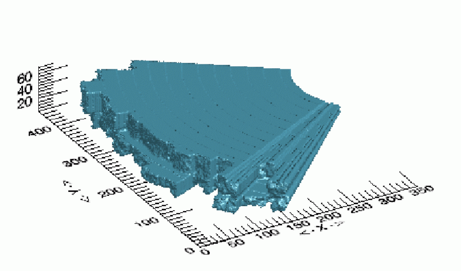
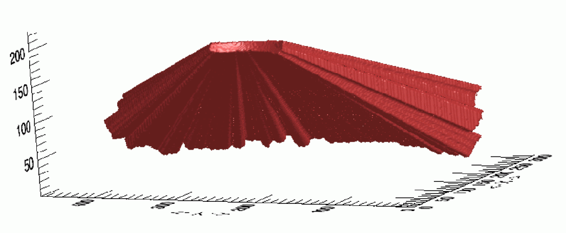
The 2dFGRS catalogue is composed of measurements in a large number of circular patches in the sky, and its footprint in the sky is relatively complex (see the survey web-page http://www.mso.anu.au/2dFGRS). Furthermore, due to the variations in the final magnitude limit used, the catalogue depth is also a function of the direction. In order to use all the data for wavelet and morphological analysis, we had to create a spatial mask, separating the sample volume from regions outside. We did it by creating first a spatial grid for a brick that surrounded the observed catalogue volume, calculated the sky coordinates for all vertices of the brick, and used then the software provided by the 2dFGRS team to find the correction factors for these directions. The completeness factor told us if the direction was inside the sample footpath. If it was, we found the apparent magnitude of the brightest galaxies (with $M=M_{\mbox{\scriptsize min}}$) of our sample for that distance and checked, if it was lower than the sample limit. If it was, the grid point was included in the mask. For the last comparison we had to change from the comoving grid distance to the luminosity distance. We assumed the $\Omega_{M}=0.3$, $\Omega_{\Lambda}=0.7$ cosmology for that and interpolated a tabulated relation between the two distances. As explained in Norberg et al. (2002), the 2dF volume-limited samples were built using the $k+e$-correction as dependent on the spectral type of a galaxy. We do not have such a quantity for the mask, so we tuned a little the bright absolute magnitude limit, checking that the mask should extend as far as the galaxy sample. For that, we had to increase the effective bright absolute magnitude limit by $\Delta M=0.25$. The nearby regions of the mask were cut off at the nearest distance limit for the observational sample.

The original survey mask in the sky includes holes around bright stars; these holes generate narrow tunnels through our spatial mask. As the masks have a complex geometry, we did not want to add discreteness effects due to resolving such tunnels. We filled them in by counting the number of neighbours in a $3^{3}$ cube around non-mask points and, if the neighbour number was larger than a chosen limit, assigning the points to the mask. We chose the required number $n$ of neighbours to avoid filling in at flat mask borders ($n=9$ is enough for that) and iterated the procedure until the tunnels disappeared. This was determined by visual checks (using the ’ds9’ fits file viewer (Joye & Mandel, 2003)).

We show the 3-D views of our masks in Fig. 5. The mask volumes are, in general, relatively thin curved slices with heavily corrugated outer walls. These corrugations are caused by the unobserved survey fields. Also, the outer edges of the mask are uneven, due to the variations in the survey magnitude limit. One 3-D view does not give a good impression of the mask; the slices we shall show below will complement these.

As mentioned in Appendix A, in order to apply the wavelet convolution cascade, the initial density on the grid should be extirpolated by the chosen scaling function. We chose our initial grid step as 1 Mpc/$h$, and used the $B^{(3)}_{3}$ kernel for extirpolation. In order to have a better scale coverage, we repeated the analysis, using the grid step $\sqrt{2}$ Mpc/$h$. The smoothing scale (the spatial extent of the kernel) is 4 grid units, the smoothing radius corresponds to 2 units. When calculating the densities, we used the spectroscopic completeness corrections $c_{\mbox{i\scriptsize sp}}$, included in the 2dFGRS volume-limited catalogues, and weighted the galaxies by the factor $w=1/c_{\mbox{i\scriptsize sp}}$. Most of the weights are close to unity, but a few of them are large. In order not to ’overweight’ these galaxies, we fixed the maximum weight level as $w=2$. The same procedure was chosen by Croton et al. (2004a).

4 Gaussian fields

The filters used to perform wavelet expansion are linear, and thus should keep the morphological structure of Gaussian fields; the Minkowski functionals should be Gaussian for any wavelet order. This is certainly true for periodic densities, but for densities restricted to finite volumes the boundary conditions can introduce correlations. The most popular boundary condition – reflection at the boundary – will keep the density field mostly Gaussian for brick masks. Our adopted zero boundary condition will certainly work destroying Gaussianity, as the random field which is zero outside a given volume and has finite values inside is certainly not Gaussian.

Figure 6: Densities of the Minkowski functionals (from the second at the left until the fourth at the right) for the same Gaussian realization for the wavelet orders 3 and 4 (lower wavelet orders give higher amplitudes). The case for the wavelets generated using the mirror boundary conditions is shown by full lines, for zero boundary conditions dotted lines are used. The amplitudes of the functionals for the wavelet order 4 are rescaled by 2 for $v_{2}$ and by 4 for $v_{3}$ to show more details.

   
   

Figure 7: Multi-scale decomposition of a realization of a Gaussian random field in the 2df19N volume mask, for the $z=34$ Mpc/$h$ slice (the data and the first orders). The upper panel column shows the scaling orders, with the original density at the right. The lower panel shows the wavelet orders, with the lowest order at the right.

   
   

Figure 8: Multi-scale decomposition of of a Gaussian random field in the 2df19N volume mask (continued). Upper panel – scaling orders, lower panel – wavelet orders, the highest orders at the left. The last scaling solution shows already strong effects of the boundary conditions.

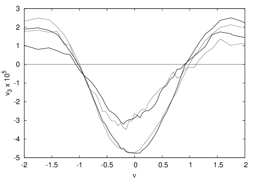
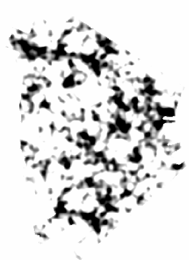
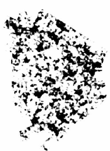
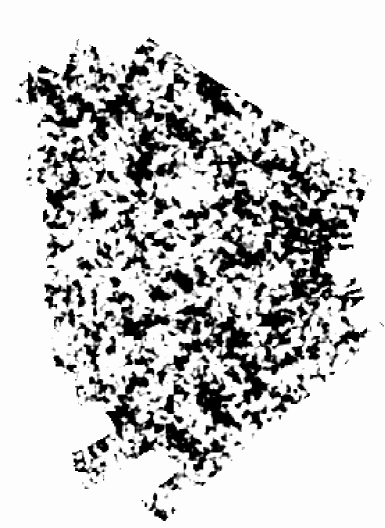
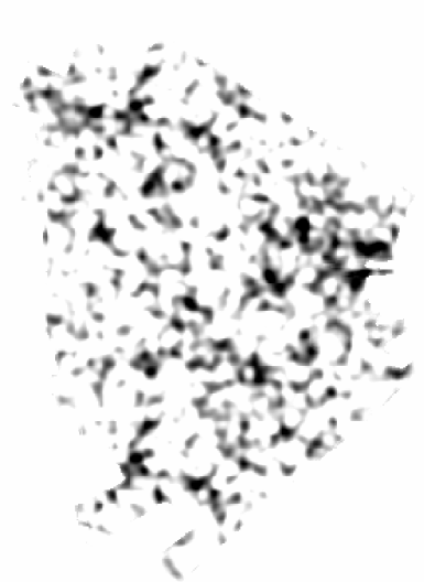
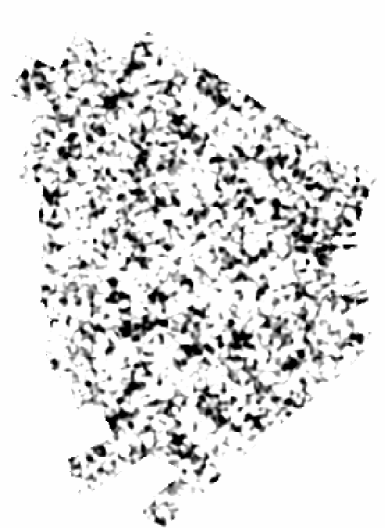
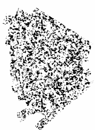
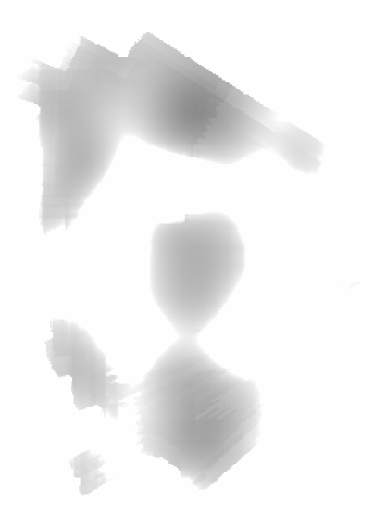
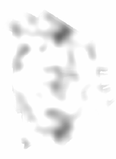
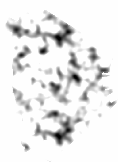
We compare the effect of the mirror and zero boundary conditions in Fig. 6, for high wavelet orders that are yet not dominated by noise, calculated for a Gaussian realization in a $256^{3}$ cube with the $\sigma=3$ Gaussian smoothing described above, and masked at all borders by a layer two vertices thick (thus the effective volume of the data cube is $252^{3}$)

Fig. 6 shows that the second Minkowski functional is certainly better restored by the wavelets obtained by using mirror boundary conditions. These conditions lead to the functionals that are symmetric about $\nu=0$, as it should be, while the functionals obtained by applying zero boundary conditions display a shift towards smaller values of $\nu$. However, although our brick data should prefer mirror boundary conditions, it is not easy to say which boundary conditions give better estimates for the remaining two functionals. Both cases have comparable errors (look at the amplitudes at extrema, which should be equal). Hence, other considerations have to be used. As our data mask is complex, with corrugated planes and sharp corners, the mirror boundary conditions will amplify the corner densities and propagate them inside, while the zero boundary conditions will gradually remove the influence of the boundary data. Thus we have selected zero boundary conditions for the present study; these are probably natural for all observational samples.

Figure 9: The density $v_{3}$ of the fourth MF for the wavelet decomposition of a realization of a Gaussian random field in the 2dfN19 mask. The legends in the figure show the wavelet order and the scaling factor (2W1 denotes the functional for the wavelet order 1, multiplied by 2). The legend NG denotes the original realization.

   
   

Figure 10: Multi-scale decomposition of the 2df19N volume-limited sample, for the $z=39$ Mpc/$h$ slice, and for the grid step $\sqrt{2}$ Mpc/$h$. The original density is shown at top right, the last scaling order at bottom left, the wavelet orders in between. The wavelet orders increase from right to left and from top to bottom. The weakest gray level shows the sample mask.

   
   

Figure 11: Multi-scale decomposition of the 2df19S volume-limited sample, for the $z=97$ Mpc/$h$ slice, and for the grid step $\sqrt{2}$ Mpc/$h$. The original density is shown at top right, the last scaling order at bottom left, the wavelet orders in between. The wavelet orders increase from right to left and from top to bottom. The weakest gray level shows the sample mask (in most cases; sometimes the mask is missing and sometimes the gray level is wider than the mask).

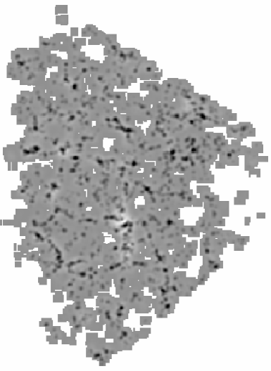
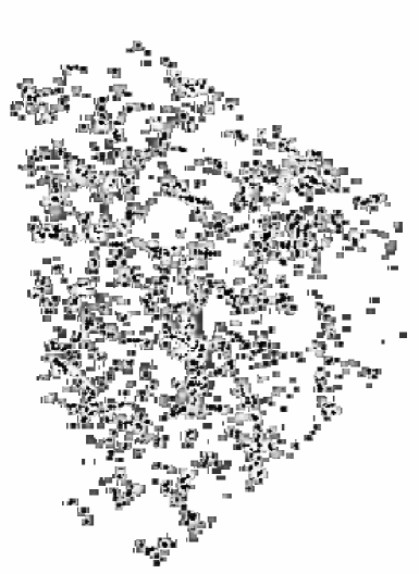
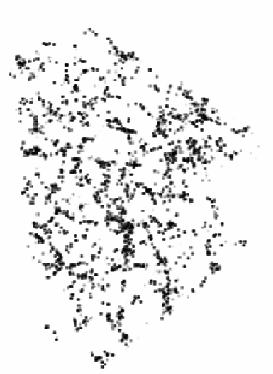
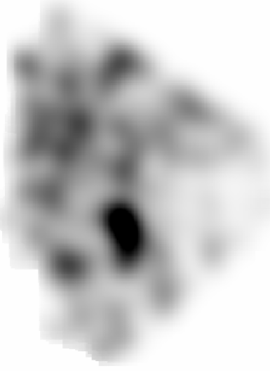
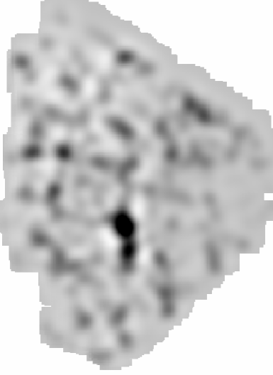
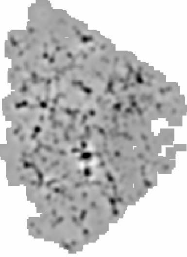
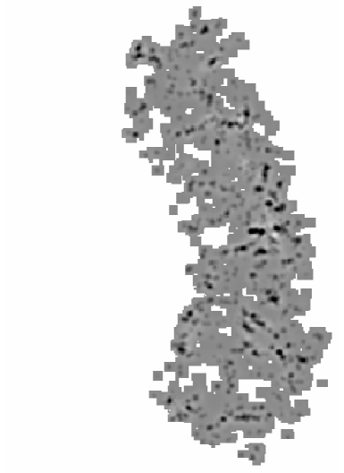
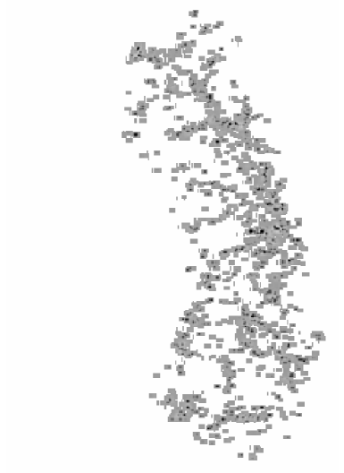
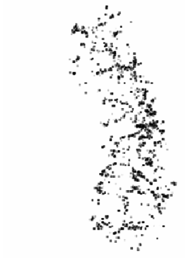
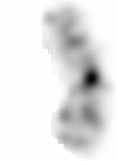
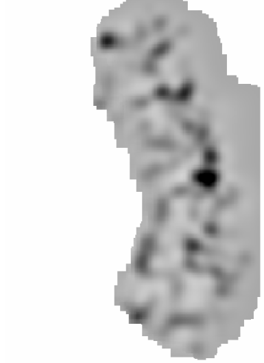
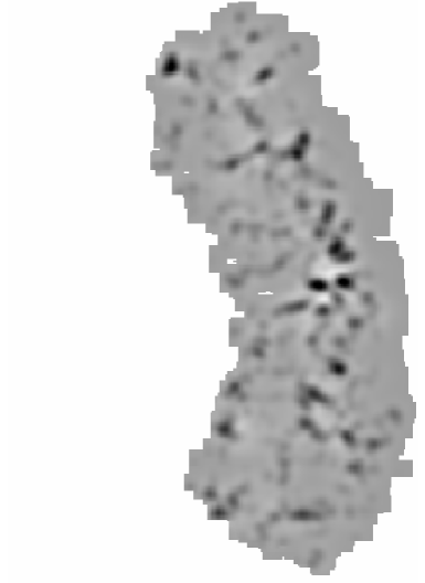
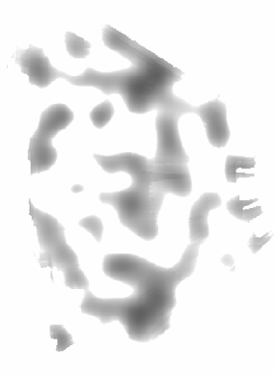
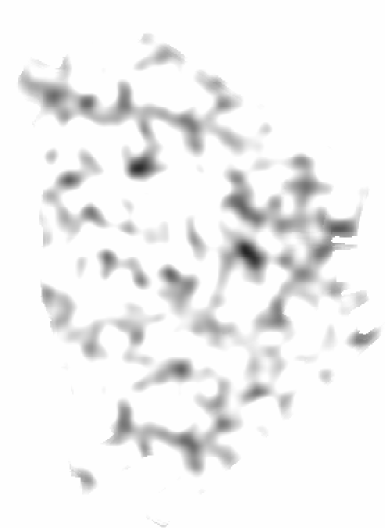
We have seen that the wavelet components of the multi-scale decomposition of a realization of a Gaussian random field remain practically Gaussian for simple sample boundaries. This means that testing for Gaussianity is straightforward. However, we have to assess the boundary effect for our application, where the boundaries are extremely complex. We shall demonstrate it on the example of the Northern mask. For that, we generated a realization of a Gaussian random field for a volume encompassing the mask, as described in section 3, and masked out the region outside the NGP data volume. As we want to see the effects that could show up in the data, we used the standard dark matter power spectrum for the $\Lambda$CDM cosmology (Klypin & Holtzman, 1997), for the cosmological parameters $\Omega_{0}=0.3,\Omega_{\Lambda}=0.7,\Omega_{\mbox{\scriptsize bar}}=0.026,h=0.7$ (this is pretty close to the standard ’concordance’ power spectrum), generated the realization on a grid with the step of 1 Mpc/$h$, and smoothed the field with a Gaussian of $\sigma=2$ Mpc/$h$. The original density distribution, the scaling distributions and the wavelets are shown in Figs. 7 and 8 for a slice at $z=34$ Mpc/$h$, at about the middle of the sample volume.

The Minkowski functional $V_{3}$ for the wavelets is shown in Fig. 9. In order not to overcrowd the figure, we do not show the theoretical predictions. The functional has been rescaled to show all functionals together in a single diagram and scaling factors are shown in the labels.

As we see, the lower the wavelet order, the larger values of $V_{3}$ are obtained (this is also true for the other functionals); this is expected, as higher orders represent increasingly smoother details of the field. The values of the functionals for the zero-order wavelet are always higher than those for the full field, as it includes only the high-resolution details that the iso-levels have to follow. Also, we have seen that the lower the order of the functional, the smaller are the distortions from Gaussianity.

The distortions of the third Minkowski functional are the largest. The functional for the zeroth-order wavelet (curve W0 in Fig. 9) shows argument compression, the result of insufficient spatial resolution of the smallest details of the field. The functional for the first-order wavelet is close to Gaussian, as is the functional for the total realization, but the second-order curve 8W2 shows strong distortions, due to a small number of independent resolution elements in the volume, and to the small height of the slice. The characteristic volume of these elements is $(4\times 2^{2})^{3}=4096$ Mpc${}^{3}/h^{3}$, and their number is about 670. The functional for the third wavelet order is already completely dominated by noise.

So, we can estimate Minkowski functionals with a high precision, and the border corrections work well. The most difficult part at the moment is the scale separation in observed samples. The sample geometries are yet slice-like, limiting the range of useful scales by the mean thickness of the slice. Complex sample borders are also a nuisance when applying the wavelet cascade. In order to take account of these difficulties, we have yet to resort to running Monte-Carlo simulations of Gaussian realizations of a right power spectrum, and to compare the obtained distributions of the functionals with the functionals for the galaxy data. We hope that for the future surveys (e.g., the full SDSS), the data volume will be large enough to do without Monte-Carlo runs.

5 Morphology of the 2dF19 sample

Having developed all necessary tools, we apply them to the 2dF19 volume-limited sample, separately for the NGC and SGC regions.

We show selected slices for the two subsamples, first (Figs. 10–11). The Northern slice was chosen to show the richest super-cluster in the 2dfGRS NGC, super-cluster 126 (middle and low, (Einasto et al., 1997)). The Southern slice has the maximum area in the $z=\mbox{const}$ slices of this sample. We choose the gray levels to show also the mask area.

Figure 12: Summary of the densities of the fourth MF $v_{3}$ for the data and all wavelet orders for the 2dFN19 sample (left) and 2dFS19 sample (right), in the logn mapping – the higher the wavelet order (indicated by labels), the lower the density amplitude. Thick lines show reference Gaussian predictions. Thin lines stand for the $\sqrt{2}$ Mpc/$h$ grid.

Figs. 12–15 show the results – the Minkowski functionals for the wavelet decompositions of the 2dFN19 and 2dFS19 subsamples.

First, we show the summary figures: the density $v_{3}$ for the original data and for wavelet orders from 0 to 3, and for grid unit of $\sqrt{2}$ Mpc/$h$. Higher wavelet orders are not usable – there the boundary rules used for the wavelet cascade influence strongly the results, and the number of independent resolution elements becomes very small, letting the functionals to be dominated by noise. The wavelet orders used span the scale range 2–22.6 Mpc/$h$. In order to show all the densities in the same plot, we use the mapping

$$\mbox{logn}(v_{3})=\mbox{sgn}(v_{3})\log(1+|v_{3}|).$$

It is almost linear for $|v_{3}|<1$, logarithmic for $|v_{3}|>1$, and can be applied to negative arguments, also. The density in Fig. 12 is shown with dotted lines. For reference, the two thick lines show the Gaussian predictions for small and large functional density amplitudes for the logn($v_{3}$) mapping. The first glance at the figures of the fourth Minkowski functional reveals that none of the wavelet scales shows Gaussian behavior.

In order to estimate the spread in the values of the functionals, we ran about 100 Gaussian realizations for every sample and grid, generated wavelets and found the Minkowski functionals. The power spectrum for these realizations was chosen as described in Sec. 4 above (see Klypin & Holtzman (1997)), and smoothed by a Gaussian of $\sigma=1$ (in grid units). This is practically equivalent to the $B_{3}$ extirpolation used to generate the observed density on the grid. Now, if the observational MF-s lie outside the limiting values of these realizations, we can say that the Gaussian hypothesis is rejected with the $p$-value less than 1%. We also calculated the multiscale functionals for a set of 22 mock samples, specially created for the 2dFGRS Norberg et al. (2002). The mock catalogs were extracted from the Virgo Consortium $\Lambda$CDM Hubble volume simulation, and a biasing scheme described in Cole et al. (1998) was used to populate the dark matter distribution with galaxies.

Fig. 13 and  14 show respectively the densities of the fourth Minkowski functional for the Northern and the Southern Galactic caps. The MF density $v_{3}$ corresponding to the data is plotted with a continuous line while error bars correspond to the total variation for mocks. The minimum and maximum limits for Gaussian realizations are plotted with dotted lines.

The Gaussian realizations show very small spread, and are clearly different from the $v_{3}$ Minkowski Functional of the observational samples. Results from mocks are much closer to the data.

Fig. 13 shows clear non-Gaussianity for the north galactic cap at a high confidence level. Gaussian realizations are not much deformed by the combination of boundary conditions (wavelets) and border corrections (functionals) effects. In this figure we can appreciate that with respect to this MF, mocks follow data well for smaller density iso-levels, but deviate around $\nu=1$; we have seen similar effects before (Martínez et al., 2005). An interesting detail is the knee around $\nu=0.5$, seen both in the data and in the mocks, but not for Gaussian realizations. The latter fact tells us that it is not caused by the specific geometry of the data sample. The grid step was 1Mpc/$h$.

Figure 13: The density of the fourth MF $v_{3}$ for the wavelet order 2 for the 2dFN19 sample (full line). Dotted lines show the minima and maxima of 102 Gaussian realizations, and bars show the full variation in a sample of 22 mock catalogues.

Figure 14: The density of the fourth MF $v_{3}$ for the wavelet order 2 (grid $\sqrt{2}$) for the 2dFS19 sample (full line). Dotted lines show the minima and maxima of 108 Gaussian realizations, and bars show the full variation in a sample of 22 mock catalogues.

Figure 15: The densities of the fourth MF $v_{3}$ for the wavelet order 1 for the 2dFS19 and 2dFN19 samples (full lines). Bars show the full variation in two samples of 22 mock catalogues.

Fig. 14 for the Southern data shows also clear non-Gaussianity, but no strong features like the northern one (it describes larger scales, as this wavelet is based on the $\sqrt{2}$ Mpc/$h$ step grid). An interesting point is that mocks follow the data curve almost perfectly here, much better than for the Northern sample.

Fig. 15 shows the $v_{3}$ MF density at the first wavelet scale for both north and south slices. Again, it is clearly non-Gaussian. However, it is remarkable how well the functionals for both volumes coincide. This shows that the border and boundary effects are small, and we are seeing real features in the density distribution that we have to explain. Also, the mocks follow the data rather well. This means that the structure (and galaxy) formation recipes used to build the mocks already implicitly include mechanisms responsible for these features.

It is useful to compare our results with the recent careful analysis of the topology of the SDSS galaxy distribution by Park et al. (2005). They used Gaussian kernels to find the density distribution, and as a result, their genus curves (see, e.g., their Figs. 6 and 8) are close to those of Gaussian fields. They describe deviations from Gaussianity by moments of the genus curve, taken in carefully chosen $\nu$ intervals, and normalized by corresponding Gaussian values. Our Minkowski functionals differ so much from Gaussian templates (see Fig. 12) that we cannot fit a reference Gaussian curve. The only analogue we can find is the shift of the genus curve $\Delta\nu$, that we estimate by fitting an expression $v_{3}(\nu)=A\left((\nu-\Delta\nu)^{2}-1\right)\exp\left(-(\nu-\Delta\nu)^{2}/2\right)$ to our results. The values of the shift corroborate the visual impression of strong differences between our results and those of Park et al. (2005). While they find that $\Delta\nu$ lies in the interval $[-0.1,0.26]$ (for the scale range $R_{G}\in[4.5,11.0]$ Mpc/$h$, their table 2), our $\Delta\nu$ assumes values between $-1.3$ and $-0.2$, for approximately the same scale interval ($\lambda\in[4,22.6]$ Mpc/$h$). As the morphology of the 2dFGRS and the SDSS should not differ much, the difference is clearly caused by different kernels, Gaussians compared to compact wavelets. Dropping the conventional Gaussian kernels makes the discriminative force of the morphological tests considerably stronger.

6 Conclusions

The main results of this paper are:

1. We have shown how to compute the MF, taking into account both the biases due to the discrete grid from the Crofton method and the border effects related to complex observational sample volumes.

2. Our experiments have shown that the multiscale MF functionals of a Gaussian Random Field have always a Gaussian behavior, even in case where the field lies within complex boundaries. Therefore, we have established a solid base for calculating the Minkowski functionals for real data sets and their multi-scale decompositions.

3. We found that both the observed galaxy density fields and mocks show clear non-Gaussian features of the morphological descriptors over the whole scale range we have considered. For smaller scales, this non-Gaussianity of the present cosmological fields should be expected, but it has been an elusive quality, not detected in most of previous papers (see, e.g., Hoyle et al. (2002), Park et al. (2005)). But even for the largest scales that the data allows us to study (about 20 Mpc/$h$), the density fields are yet not Gaussian. We believe that the Gaussianity reported in the papers cited above could be just a consequence of oversmoothing the data. This effect was clearly described in Martínez et al. (2005).

4. The mocks that are generated from initial Gaussian density perturbations by gravitational evolution and by applying semi-analytic galaxy formation recipes, are pretty close to the data. However, as in a previous study (Martínez et al., 2005), we confirm a discrepancy around $\nu=1$ between the mocks and the data. This analysis clearly shows that there are more faint structures in the data than in the mocks, and clusters in the mocks have a larger intensity than in the real data.

Appendix A: The à trous algorithm and galaxy catalogues

A good description of the à trous algorithm and of its applications to image processing in astronomy can be found in Starck & Murtagh (2002). Readers interested in the mathematical basis of the algorithm can consult Mallat (1999) and Shensa (1992). We give below a short summary of the algorithm and describe the additional intricacies that arise when the algorithm is applied to galaxy catalogues (point data).

We start with forming the initial density distribution $d_{0}$ on a grid. In order to form the discrete distribution, we have to weight the point data (extirpolate), using the scaling kernel for the wavelet (Mallat, 1999). As we shall use the $B_{3}$ box spline as the scaling kernel, the extirpolation step is:

$$d^{(0)}(\mathbf{n}_{i})=\int\rho(\mathbf{x})B_{3}^{(3)}(\mathbf{x-n}_{i})d^{3}x,$$ (11)

where $\mathbf{n}_{i}\equiv(n)_{i}=(x_{i},y_{i},z_{i})$ is a grid vertex, $\rho(\mathbf{x})$ is the original density, delta-valued at galaxy positions, and $B_{3}^{(3)}(\mathbf{x})$ is the direct product of three $B_{3}$ splines:

$$B_{3}^{(3)}(\mathbf{x})=B_{3}(x)B_{3}(y)B_{3}(z),$$

where $\mathbf{(}x)=(x,y,z)$. The $B_{3}$ spline is given by

$$B_{3}(x)=\frac{1}{12}\left[|x-2|^{3}-4|x-1|^{3}+6|x|^{3}-4|x+1|^{3}+|x+2|^{3}\right].$$

As this function is zero outside the cube $[-2,2]^{3}$, every data point contributes only to its immediate grid neighbourhood, and extirpolation is fast.

The main computation cycle starts now by convoluting the data $d$ with a specially chosen discrete filter $h_{(k)}$:

$$d^{(I+1)}_{(n)}=\sum_{(k)}h_{(k)}d^{(I)}_{(n)+2^{I}(k)}.$$ (12)

Here $I$ stands for the convolution order (octave), the 3-dimensional filter $h_{(k)}=h_{l}h_{m}h_{n}$, $(k)=(l,m,n)$ is the direct product of three one-dimensional filters $h_{i}=\{1/16,1/4,$ $3/8,1/4,1/16\}$, for $i\in[-2,2]$. Two points should be noted:

• As the filter is the direct product of the one-dimensional filters, the convolution can be applied consecutively for each coordinate, and can be done in place, with extra memory only for a data line.

• The data index $(n)+2^{I}(k)$ in the convolution shows that the data is assessed from consecutively larger regions for further octaves, leaving intermediate grid vertices unused. This is equivalent to inserting zeroes in the filter for these points, and this is where the name of the method comes from (à trous is “with holes” in French). This makes the convolution very fast, as the number of operations does not increase when the filter width increases.

The filter $h_{i}$ is satisfies the dilation equation

$$\frac{1}{2}B_{3}\left(\frac{x}{2}\right)=\sum_{k}h_{k}B_{3}(x-k).$$

After we have performed the convolution (12), we find the wavelet coefficients $w^{(J)}$ for the octave $J$ by simple substraction:

$$w^{(J)}_{(n)}=d^{(J)}_{(n)}-d^{(J+1)}_{(n)}.$$ (13)

The combination of steps (12,13) is equivalent to convolution of the data with the associated wavelet $\psi^{(3)}(x)$, where

$$\psi(x)=2B_{3}(2x)-B_{3}(x).$$ (14)

Repeating the sequence (12,13) we find wavelet coefficients for a sequence of octaves. The number of octaves is, evidently, limited by the grid size, and in real applications by the geometry of the sample.

We have illustrated the wavelet cascade in the main text by application to real galaxy samples. As our wavelet amplitudes were obtained by subtraction, we can easily reconstruct the initial density:

$$d^{(0)}_{(n)}=d^{(J+1)}_{(n)}+\sum_{j=0}^{j=J}w^{(j)}_{(n)}.$$ (15)

Here the upper indices show the octave, the lower indices denote grid vertices, and $d^{(J+1)}$ is the result of the last convolution. This formula can also be interpreted as the decomposition of the original data (density field) into contributions from different scales – the wavelet octaves describe contributions from a limited (dyadic) range of scales.

Here we have to note that while the scaling kernel

$$\Phi(x,y,z)=B_{3}(x)B_{3}(y)B_{3}(z)$$

is a direct product of three one-dimensional functions, it is surprisingly almost isotropic. Its innermost iso-levels are slightly concave, and outer iso-levels tend to be cubic, but this happens at very low function values. In order to characterise the deviation from anisotropy, let us first define the angle-averaged scaling kernel

$$\bar{\Phi}(r)=\frac{1}{4\pi}\int_{S}(r)\Phi(r,\theta,\phi)dS,$$

where $S(r)$ is a spherical surface of a radius $r$. The anisotropy can now be calculated as the integral of the absolute value of the difference between the kernel and its angle-averaged value:

$$\int_{2}^{2}\int_{2}^{2}\int_{2}^{2}\left|\Phi(x,y,z)-\bar{\Phi}(\sqrt{x^{2}+y^{2}+z^{2}})\right|\,dx\,dy\,dz=0.030.$$

As the integral of the kernel itself is unity, the deviation is only a couple of per cent.

A similar integral over the wavelet profile gives the value 0.052. Here the natural scale, the integral of the square of the wavelet profile, is also unity, so the deviation from isotropy is small.

Isotropy of the wavelet is essential, if we want to be sure that our results do not depend on the orientation of the grid. This is usually assumed, but with a different choice of the scaling kernel this could easily happen.

As our wavelet transform is not orthogonal, there remain correlations between wavelet amplitudes of different octaves. The Fourier transform of the $B_{3}$ scaling function is

$$\hat{B}_{3}(\omega)=\left(\frac{\sin(\omega/2)}{\omega/2}\right)^{4}$$

The Fourier transform of the associated wavelet (13) is

$$\hat{w}(\omega)=\hat{B}_{3}(\omega/2)-\hat{B}_{3}(\omega).$$

Figure 16: The square of the Fourier transform of the wavelet for two neighbouring octaves.

We show the square of the Fourier transform of the wavelet for two neighbouring octaves in Fig. 16. As we see, the overlap between the octaves is not large, but substantial. This is the price we pay for keeping the wavelet transform shift invariant. We can now compare wavelet amplitudes for different octaves (scale ranges) at any grid vertex, but we have to keep in mind that the separation of scales is not complete. It may seem an unpleasant restriction that the wavelet scales have to increase in dyadic steps. It is not, in fact, as one can choose the starting scale (the step of the grid) at will.

Before applying the wavelet transform to the data, we have to decide how to calculate the convolution (12) near the spatial boundaries of the sample. Exact convolution can be carried out only for periodic test data, and spatially limited data need special consideration. For density estimation, a useful method to deal with boundaries is to renormalise the kernel. This cannot be done here, as renormalisation would destroy the wavelet nature of our convolution cascade. The only assumptions that can be used are those about the behaviour of the density outside the boundaries of the sample. Let us consider, for example, the one-dimensional case and the data $d(i)$ known only for the grid indices $i>0$. The possible boundary conditions are, then:

$$d(i;i<0)=\left\{\begin{array}[]{r@{\quad:\quad}l}0&\mbox{zero boundary}\\ d(0)&\mbox{constant boundary}\\ d(-i)&\mbox{reflecting boundary}.\end{array}\right.$$

The constant boundary condition is rarely used; the most popular case seems to be the reflecting boundary. For brick-type sample geometries, where the coordinate lines are perpendicular to the sample boundary, this condition gives good results. However, in our case the sample boundary has a complex geometry, and reflections from nearby boundary surface details would soon interfere with each other.

Appendix B. Comparing border corrections

Figure 17: Relative errors of border-corrected densities of the second MF $v_{1}$ for a realization of a Gaussian random field in the 2df19N sample mask. The case of the border correction chain is shown by solid line, the ’raw’ correction case – by dotted line.

We noted above (Sec. 2.4) that alongside with the border correction chain (2.4) there is another possibility to correct for borders. In this case we ignore the vertices in the mask and do not build any basic elements if one of the vertices belong to the mask. This also means that we do not have to build the basic elements in the mask region. The latter fact makes the algorithm faster (about twice faster for the 2dF data), as the data region occupies usually only a fraction of the encompassing brick).

Figure 18: Relative errors of border-corrected densities of the third MF $v_{2}$ for a realization of a Gaussian random field in the 2df19N sample mask. The case of the border correction chain is shown by solid line, the ’raw’ correction case – by dotted line.

We call this method the ’raw’ border correction and compare it with the border-correction algorithm (2.4) on the example of the realization of a Gaussian random field for the 2dF NGC region, smoothed by a Gaussian of $\sigma=3$ Mpc/$h$ to ensure that we resolve the density distribution. (We used the same realization to compare the border-corrected and uncorrected case, in Sec. 2.4.) We combine the encompassing Gaussian brick with the 2dFN19 mask, calculate the Minkowski functionals for both border correction methods, and compare them with the functionals found for the periodic brick. We show below the relative errors of the functionals, defined as

$$\varepsilon(v_{i}(\nu))=\frac{v_{i}(\nu)-v^{b}_{i}(\nu)}{\max_{\nu}|v^{b}_{i}(\nu)|},$$

where $v^{b}_{i}(\nu)$ are the densities of the functionals for the brick. We cannot use $v^{b}_{i}(\nu)$ themselves to normalise the errors, as their values pass through zero, so we use their maximum absolute values.

Figure 19: Relative errors of border-corrected densities of the fourth MF $v_{3}$ for a realization of a Gaussian random field in the 2df19N sample mask. The case of the border correction chain is shown by solid line, the ’raw’ correction case – by dotted line.

The relative differences are shown in Figs. 17-19. We see that both correcting methods give the results that do not differ from the true densities more than 10% (12% for $v_{3}$). We see also that the border correction chain (2.4) gives always better estimates of the functionals; the maximum error is 3–4%, and the error is about three times smaller than that for the ’raw’ border correction. Thus we use this chain throughout the paper.

It is useful to recall, though, that the border corrections (2.4) are based on the assumption of homogeneity and isotropy of the data, which may not always be the case. The ’raw’ border corrections do not rely on any assumptions, and are therefore useful for verifying the results obtained by the correction chain.

References

- Adler (1981) Adler, R. J. 1981, The Geometry of Random Fields, (New York: John Wiley & Sons)
- Ascasibar & Binney (2005) Ascasibar, Y., & Binney, J., 2005, MNRAS, 356, 872
- Cole et al. (1998) Cole, S., Hatton, S., Weinberg, D. H., & Frenk, C. S., 1998, MNRAS, 300, 945.
- Coles et al. (1996) Coles, P., Davies, A. G., & Pearson, R. C. 1996, MNRAS, 281, 1375.
- Colless et al. (2003) Colless, M., et al. 2003, astro-ph/0306581.
- Croton et al. (2004a) Croton, D. J., et al. 2004, MNRAS, 352, 828
- Croton et al. (2004b) Croton, D. J., et al. 2004, MNRAS, 352, 1232
- Donoho (1988) Donoho, D. L., 1988, Ann. Statist., 16, 1390
- Einasto et al. (1997) Einasto, M., et al. 1997, A&AS, 123, 119
- Gott et al. (1986) Gott, J. R., Dickinson, M., & Melott, A. L. 1986, ApJ, 306, 341
- Hamilton et al. (1986) Hamilton, A. J. S., Gott, J. R. I., Weinberg, D. 1996, ApJ, 309, 1
- Hoyle et al. (2002) Hoyle, F., et al. 2002, ApJ, 580, 663
- Joye & Mandel (2003) Joye, W. A., & Mandel, E., 2003, ADASS XII ASP Conf. Ser.. 295, 489
- Kerscher et al. (1997) Kerscher, M., et al. 1997, MNRAS, 284, 73
- Klypin & Holtzman (1997) Klypin, A., & Holtzman J. 1997, astro-ph/9712217
- Maddox et al. (1996) Maddox, S. J., Efstathiou, G., & Sutherland, W. J. 1996, MNRAS, 283, 1227
- Mallat (1999) Mallat, S., 1999, A wavelet tour of signal processing (San Diego: Academic Press)
- Martínez et al. (1993) Martínez, V. J., Paredes, S., & Saar, E. 1993, MNRAS, 260, 365
- Martínez & Saar (2002) Martínez, V. J., & Saar, E. 2002, Statistics of the Galaxy Distribution, (Boca-Raton: Chapman & Hall/CRC press)
- Martínez et al. (2005) Martínez, V. J., et al. 2005, ApJ, 634, 744
- Mecke et al. (1994) Mecke K. R., Buchert, T., & Wagner, H. 1994, A&A, 288, 697
- Minkowski (1903) Minkowski, H., 1903, Mathematische Annalen 57, 447
- Norberg et al. (2002) Norberg, P., et al. 2002, MNRAS, 336, 907
- Park et al. (2005) Park, C., et al. 2005, ApJ, 633, 11
- Pelupessy et al. (2003) Pelupessy, F. I., Schaap, W. E., & van de Weygaert, R. 2003, A&A, 403, 389
- Sahni et al. (1998) Sahni, V., Sathyaprakash, B. S., & Shandarin, S. F., 1998, ApJ, 495, L5
- Schaap & van de Weygaert (2000) Schaap, W. E., & van de Weygaert, R., 2000, A&A, 363, L29
- Schmalzing & Buchert (1997) Schmalzing J., & Buchert, T. 1997, ApJ, 482, L1
- Schmalzing et al. (1996) Schmalzing J., Kerscher M. and Buchert T. (1996), in Dark Matter in the Universe, eds. S. Bonometto, J.R. Primack & A. Provenzale, (Amsterdam: IOS Press), 281
- Shandarin et al. (2004) Shandarin, S. F., Sheth, J. V., & Sahni, V., 2004, MNRAS, 353, 162
- Sheth & Sahni (2005) Sheth, J. V., & Sahni, V. 2005, Current Science, 88, 1101
- Sheth et al. (2003) Sheth, J. V., Sahni, V., Shandarin, S. F., & Sathyaprakash, B. S., 2003, MNRAS, 343, 22
- Shensa (1992) Shensa,M. J., 1992, IEEE Trans. Signal Proc., 40, 2464
- Starck & Murtagh (2002) Starck, J.-L., & Murtagh, F. 2002, Astronomical Image and Data Analysis, (Berlin: Springer-Verlag)
- Starck et al. (1998) Starck, J.-L., Murtagh, F. & Bijaoui, A. 1998, Image Processing and Data Analysis: The Multiscale Approach, (Cambridge: Cambridge University Press)
- Starck & Pierre (1998) Starck, J.-L., Pierre, M. 1998, A&AS, 128, 397
- Starck et al. (1995) Starck J.-L., Bijaoui, A., Murtagh, F., 1995, CVGIP: Graphical Models and Image Processing, 57, 420.
- Starck et al. (2005) Starck, J.-L., Martínez, V. J., Donoho, D. L., Levi, O., Querre, P. & Saar, E. 2005, Eurasip Journal of Signal Processing, 2005-15, 2455.
- Tomita (1990) Tomita, H., 1990, in Formation, Dynamics and Statistics of Patterns eds. K. Kawasaki, et al., Vol. 1, (World Scientific), 113
- York et al. (2000) York, D. G., et al. 2000, AJ, 120, 1579